Abstract
GNSS time-series prediction plays an important role in the monitoring of crustal plate movement, and dam or bridge deformation, and the maintenance of global or regional coordinate frames. Deep learning is a state-of-the-art approach for extracting high-level abstract features from big data without any prior knowledge. Moreover, long short-term memory (LSTM) networks are a form of recurrent neural networks that have significant potential for processing time series. In this study, a novel prediction framework was proposed by combining a multi-scale sliding window (MSSW) with LSTM. Specifically, MSSW was applied for data preprocessing to effectively extract the feature relationship at different scales and simultaneously mine the deep characteristics of the dataset. Then, multiple LSTM neural networks were used to predict and obtain the final result by weighting. To verify the performance of MSSW-LSTM, 1000 daily solutions of the XJSS station in the Up component were selected for prediction experiments. Compared with the traditional LSTM method, our results of three groups of controlled experiments showed that the RMSE value was reduced by 2.1%, 23.7%, and 20.1%, and MAE was decreased by 1.6%, 21.1%, and 22.2%, respectively. Our results showed that the MSSW-LSTM algorithm can achieve higher prediction accuracy and smaller error, and can be applied to GNSS time-series prediction.
1. Introduction
The long-term accumulated Global Navigational Satellite System (GNSS) coordinate time series provides valuable data for geodesy and geodynamic research [1,2,3]. These data not only reflect the long-term trend of change, but also represent nonlinear changes caused by geophysical effects. GNSS coordinate time series play an important role in the monitoring of crustal plate movements [4,5], dam or bridge deformation monitoring [6,7,8,9,10], and the maintenance of global or regional coordinate frames [11,12]. The coordinates of the successive time point can be predicted by analyzing the GNSS coordinate time series, thus providing an important basis for judging the motion trend. Therefore, the prediction of GNSS coordinate time series is a highly valuable work.
It is well known that the GNSS coordinate time series reflect both the deterministic law of motion and uncertain information, which may be caused by imperfect processing models, geophysical effects, and other factors that are difficult to model [13]. Two kinds of time-series analysis methods exist: physical modeling and numerical modeling. In the traditional physical and numerical modeling method, models of coordinate time series are constructed according to geophysics theory, the linear term, the periodic term, and gap information [14,15]. Usually, in these traditional modeling methods, the feature information and modeling parameters must be established artificially. The exclusion of elements will lead to systematic deviation and limitations in the results.
Deep learning is an emerging technology that forms a deep architecture by stacking learning modules in a hierarchical structure, and trains the whole network in an end-to-end manner according to gradient training. The deep learning algorithm does not need to artificially select the feature information, and automatically extracts the information suitable for the data characteristics by constructing a complex and precise network [16]. Due to the development of artificial intelligence (AI), an increasing number of powerful algorithms have been applied in different fields and have achieved excellent results. Among these, the recurrent neural network (RNN) is one of the most popular AI methods used for time-series prediction, and can process sequence information and regard the output of the current epoch as the input for the subsequent epoch [17,18]. Its data-driven characteristic can effectively memorize the information of the data. However, because the RNN is subject to the problem of the vanishing gradient, it cannot easily handle long sequences [19]. Thus, Hochreiter and Schmidhuber proposed long short-term memory (LSTM), which avoids the problem of gradient disappearance by optimizing memory cells via the use of gates [20]. LSTM has been widely used to deal with sequence learning problems such as natural language processing (NLP), and has shown significant potential for time-series prediction, such as air quality forecasting, weather forecasting, and traffic flow prediction [21,22,23].
Recently, LSTM has also been applied in the GNSS field, and has achieved remarkable results. In the monitoring of landslide deformation, Xing et al. proposed a model based on variational mode decomposition (VMD) and a stack LSTM, which had a higher forecast accuracy than that of LSTM and the EMD-LSTM network, in experiments conducted in Dashuitian [24]. Subsequently, Xing et al. combined the double moving average (DMA) method and LSTM to predict landslide displacement, and obtained high-quality confidence intervals [25]. Xie et al. used the LSTM algorithm to predict the periodic component of landslides, and showed that the performance of LSTM has good characteristics of dynamic features [26]. Wang et al. developed an attention mechanism LSTM model based on Complete Ensemble Empirical Mode Decomposition with Adaptive Noise (CEEMDAN-AMLSTM), and confirmed its validity for landslide displacement prediction [27]. Yang et al. used an LSTM model to predict the periodic displacement of landslides in the Three Gorges Reservoir Area, and found that the LSTM method can simulate the dynamic characteristics of landslides better than a static model due to full use of historical information [28].
In navigation and positioning, Tan et al. used LSTM as a de-noising filter and proposed the rEKF-LSTM method to significantly improve single-point positioning accuracy [29]. Jiang et al. proposed an LSTM-RNN algorithm to filter MEMS gyroscope outputs, and the results indicated that the method was effective for improving MEMS INS precision [30]. Kim et al. improved the accuracy and stability of GNSS absolute solutions for autonomous vehicle navigation using LSTM [31]. Tao et al. developed a CNN-LSTM method to mine the deep multipath features in GNSS coordinate series, and showed that the CNN-LSTM can effectively mitigate multi-GNSS multipath issues and reduce the average RMS of positioning errors [32]. In addition, Hoang et al. proposed an LSTM structure for WiFi fingerprinting of indoor localization, and achieved a smaller average localization error than that obtained from other algorithms [33]. Fang et al. used LSTM to support an inertial navigation system (INS), and confirmed that the algorithm can enhance the navigation accuracy compared with pure INS [34]. The above research shows that LSTM has produced good results in both deformation monitoring and positioning in the GNSS field, and the use of deep learning has gradually become more common, providing new ideas for research.
Prior to the use of LSTM, the data must be preprocessed. The traditional approach of a single sliding window is widely used in the existing research on data preprocessing. A review of studies of image processing shows that the multiscale sliding window is widely used in this area, and has achieved good results, because it can take into account information at different scales. The multiscale sliding window is a feature extraction method for image processing in the field of computer vision [35,36] that is able to consider the feature information at different scales. In this study, we applied the idea of the multiscale sliding window to one-dimensional time-series data. Furthermore, we applied the algorithm that was originally conceived for application to two-dimensional data, to one-dimensional data, thus providing a new idea for the use of LSTM.
In this study, we proposed a multiscale sliding window LSTM (MSSW-LSTM) approach for GNSS time-series prediction. The new method uses several different sliding windows for data preprocessing that can capture data information at different scales. Then, the preprocessed outputs are used as inputs into the corresponding LSTM, and each LSTM can be adjusted according to the data. The structure of this article is as follows: Section 2 details the methodology for the MSSW-LSTM. Then, the data and processing strategy are introduced in Section 3. Section 4 analyses the experimental results, and a discussion and conclusions are given in Section 5.
2. Methodology
2.1. LSTM
The traditional neural network model does not encompass the processing information of the previous time span, but only concerns information of the current time. In contrast, the RNN has a memory function, which provides information of the current moment to the subsequent moment. However, the long-term dependence of the RNN leads to gradient explosion. By comparison, LSTM can avoid the problem of gradient disappearance by optimizing memory cells, via the introduction of the concept of gates.
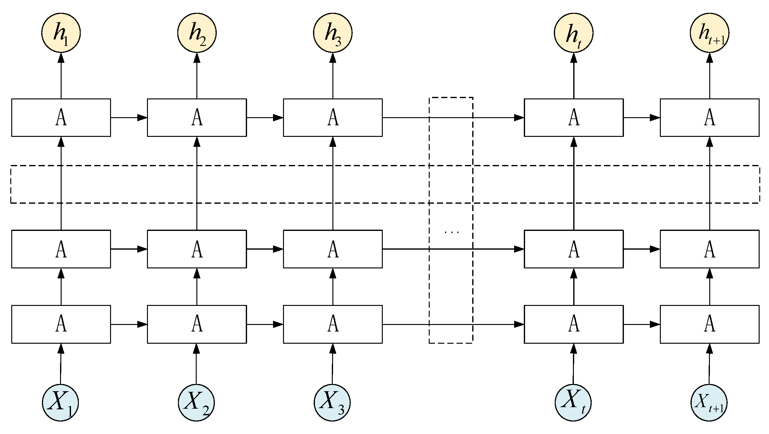
As shown in Figure 1a, a typical LSTM cell has three gates, i.e., input gate, forget gate, and output gate. The cell state and output hidden state are also cores of the LSTM cell.

Figure 1.
(a) Long short-term memory architecture; (b) typical structure of LSTM (1 layer).
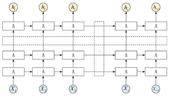
Figure 2.
Multilayered neural networks of LSTM.
The definition of the forget gate can be written as:
where is the logistic sigmoid function, , are the weight matrix for transformation of information from cell to gate vectors, is the input of the previous time, is the input of the current time, is the offset value of the forget gate, and is the forget gate of the moment . The forget gate combines the input of the previous time with the input of the current time to selectively forget the content.
The input gate can be shown as:
where and are activation functions, , , , are weight matrixes, is the input of the previous time, is the input of the current time, and are offset values of the input gate, and and are the input gates of the moment. The input gate combines the input of the previous time with the input of the current time to selectively remember the content.
The definition of the cell state update can be written as:
where is the forget gate, represents the information of the previous moment on the main line, and is the input gate. denotes information that should be memorized at time , and indicates the cell state of the main line. The main line cells selectively remember and forget the current input information. Finally, the output gate can be obtained by:
where and are activation functions, and are weight matrixes, indicates the input of the previous time, is the input of the current time, denotes offset values of the input gate, represents the output gate, is the cell state of the main line, and denotes the output of the moment.
2.2. Multi-Scale Sliding Window LSTM
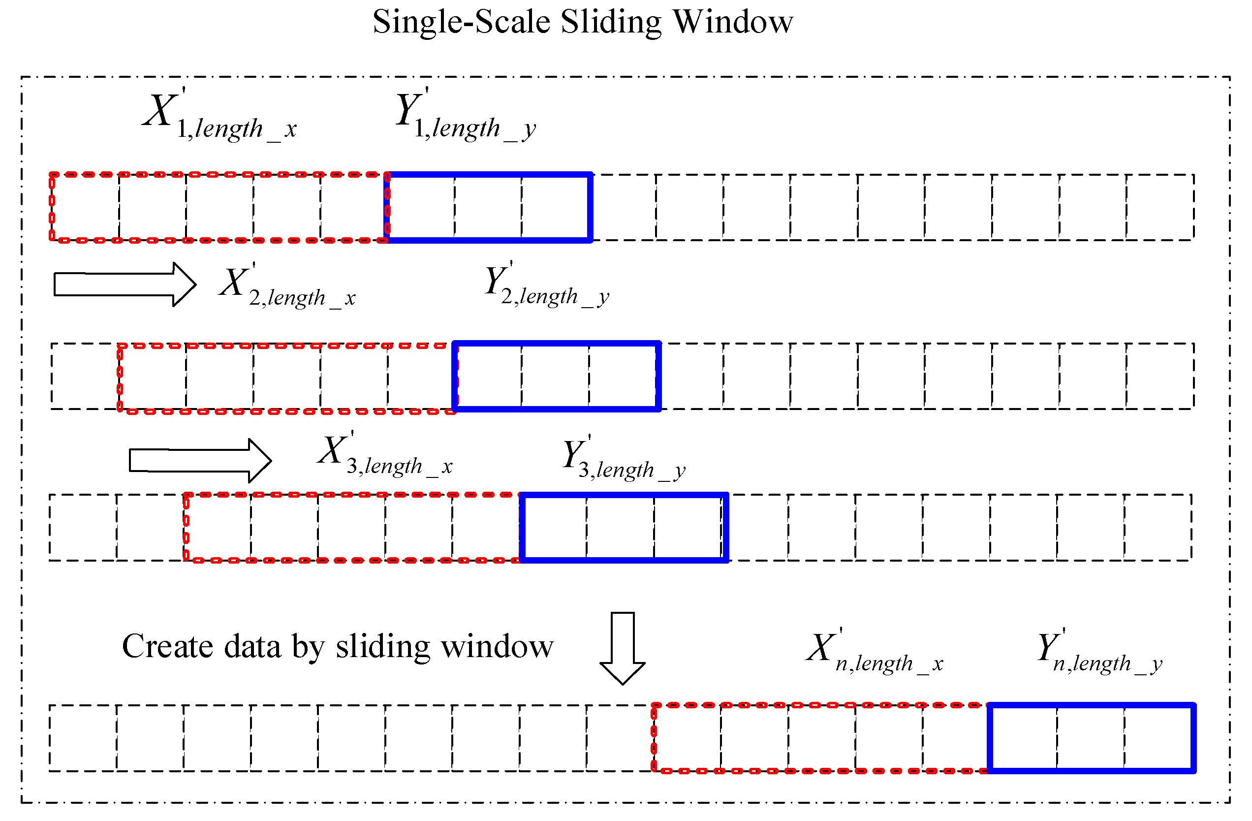
The sliding window, usually when dealing with two-dimensional images, is widely used in computer vision processing, such as in the fields of object detection and semantic segmentation. In this study, the concept of the sliding window was applied to data preprocessing. because GNSS coordinate time series are one dimensional, the sliding window was reduced to one dimension to construct the data sets. Traditional data preprocessing uses a single-scale sliding window to establish the initial data, as shown in Figure 3, among which the and are unique. The current LSTM research on time series uses a single-scale sliding window, or other transformations of the data. However, the information captured by a single scale at each time has a fixed scale, and this method of constructing a dataset is not perfect. The construction of the dataset may determine the accuracy of the model training. In this study, we proposed the method of a multiscale sliding window to input different scale information into the corresponding network, form a unified dimension, and integrate the existing research into a unified processing framework.
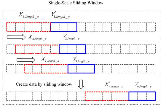
Figure 3.
Single-scale sliding window.
The GNSS coordinate time series are obtained and arranged in a unified dimension according to the time sequence:
where is the length of . The interval of the GNSS time series should a adopt uniform dimension, such as seconds, minutes, hours, days, weeks, months, or years. The construction the of multiscale sliding window is undertaken as follows:
Assume that the length of the front portion in the ith sliding window is , and the length of the back portion is . At each time, one unit is moved to sequentially construct the data, and the following conditions are required . The data formats are as follows:
In the multiscale mode, , where represents a total of scales. , , …, are not equal because it would be meaningless to construct duplicate data sets. However, , , and are equal, which is convenient for the final result of the weighting calculation.
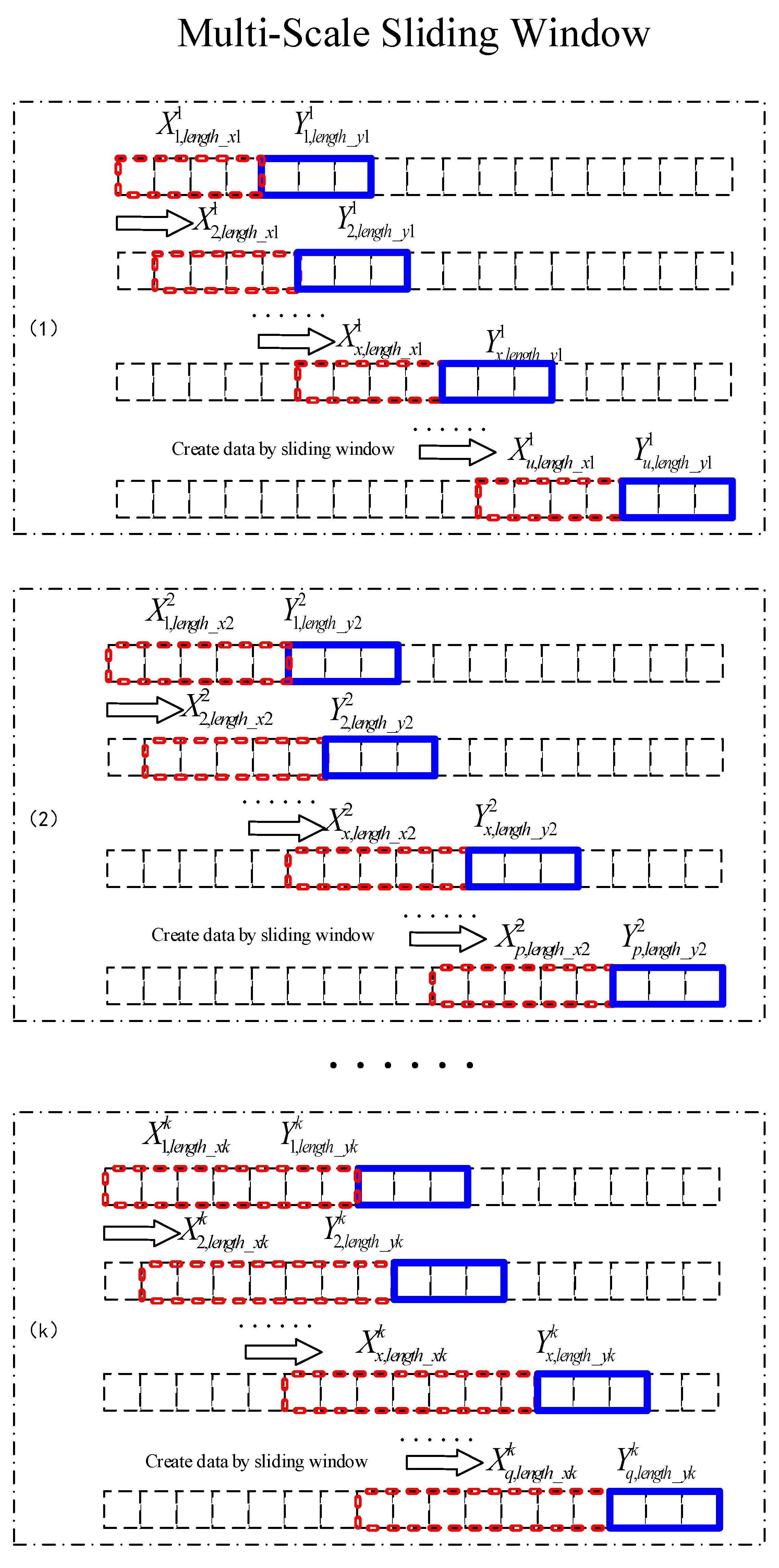
The constructed data set is shown in Equation (9) and Figure 4:
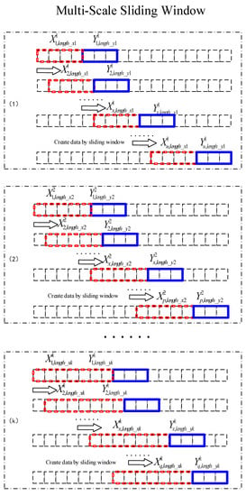
Figure 4.
Constructing data with sliding windows of different scales.
Figure 4 is a schematic diagram of K sliding windows of different scales. It can be seen that the sizes of the red sliding windows are different at different scales, and the sizes of the blue sliding windows are the same.
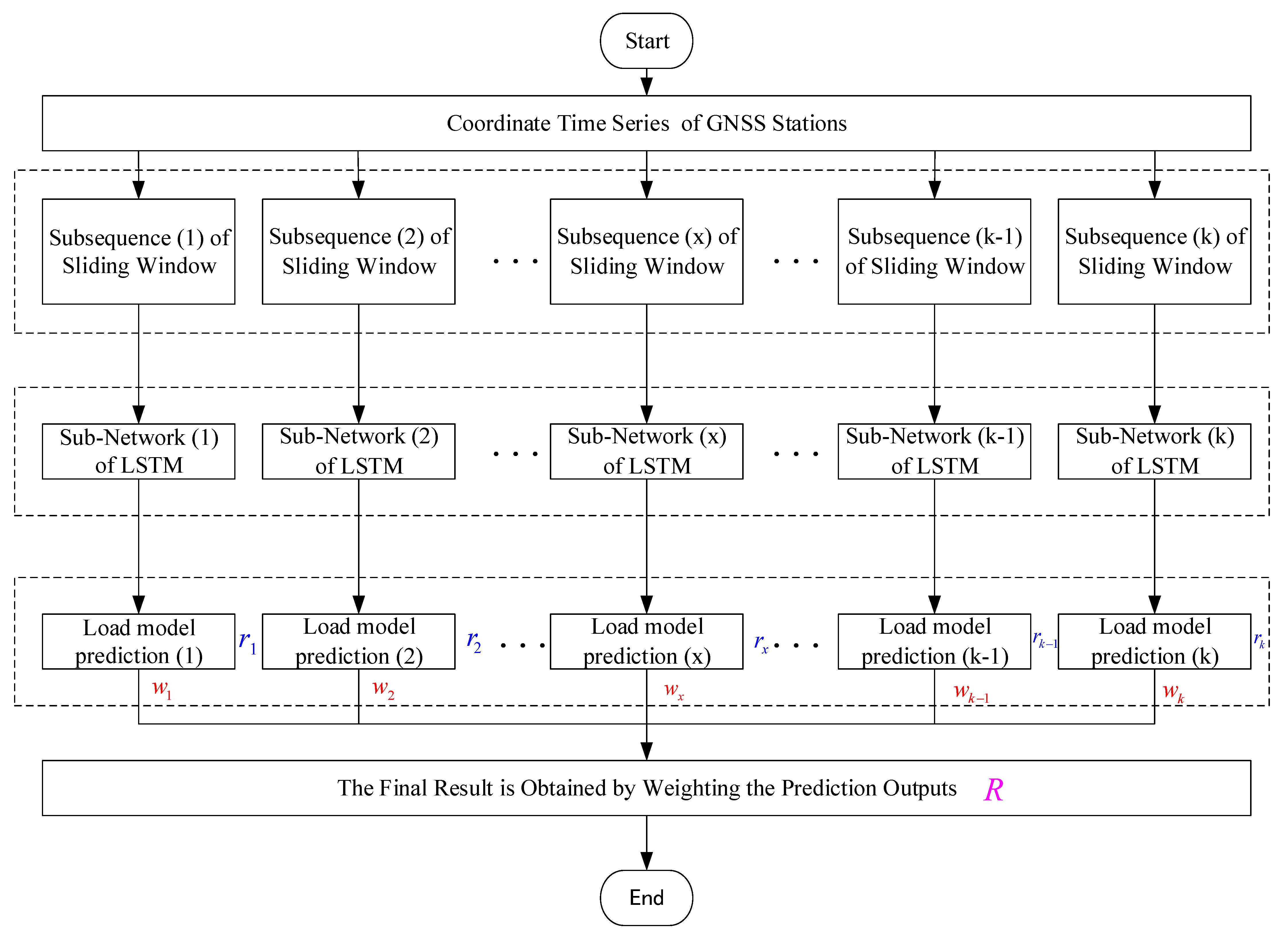
Thus, an MSSW-LSTM algorithm for GNSS time-series prediction was proposed. The overall processing flow of MSSW-LSTM is shown in Figure 5. First, the GNSS station coordinate time series is obtained, and different datasets are constructed using the multiscale window. Following the construction of the datasets, the corresponding LSTM subnetworks are established for each data set according to the actual situation of the data set.
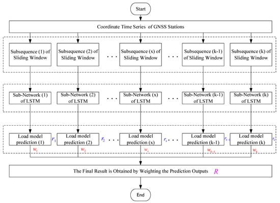
Figure 5.
Framework of the multiscale sliding window LSTM (MSSW-LSTM).
Each LSTM sub network has its own weight matrix after training, adjustment, and optimization. The trained parameters are saved, and the model of each subnetwork is used for prediction. The prediction results of each subnetwork (1) , subnetwork (2) , …, sub network (k) are then obtained.
The final prediction value is the weighted value of each subnetwork prediction result, and the calculation formula is shown in Equation (10):
where , ,…, and are the weights of the prediction results from each subnetwork. The sum of all weight values should be 1, as shown in Equation (11).
In general, if there is little difference between the subnetworks, the weight value of each subnetwork should be the same, as shown in Equation (12).
It should be noted that the MSSW-LSTM method has significant flexibility. For example, LSTM networks may be the same or different, and may consistent of a single layer or multiple layers. This flexibility is beneficial for researchers, who are able to select the most appropriate network model according to their own dataset characteristics and utilize the advantages of the network model.
2.3. Evaluation Criteria
To quantitatively evaluate the prediction accuracy of our proposed model, some indexes are used to calculate the difference between the real value and the predicted value. Here, the root mean square error (RMSE) and the mean absolute error (MAE) are used to evaluate the prediction accuracy [37], and the corresponding formulas are shown as below.
where is the number of datasets, and are true values and are predicted values.
3. Data and Processing Strategy
3.1. MSSW-LSTM Process Strategy
The data processing strategy proposed in this paper is shown in Figure 6a, and the main steps of the MSSW-LSTM algorithm are described in Table 1.
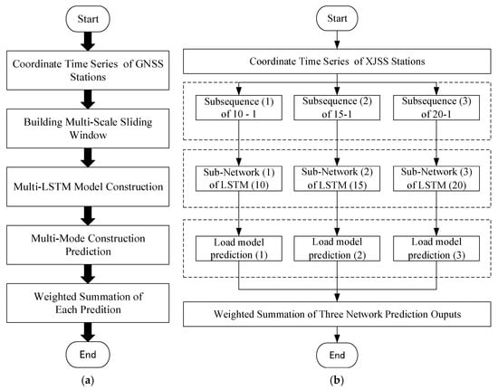
Figure 6.
(a) Flowchart of MSSW-LSTM; (b) data processing of XJSS using MSSW-LSTM.

Table 1.
Training the MSSW-LSTM algorithm.
Figure 6b shows the specific method of using the MSSW-LSTM algorithm to process the XJSS station. Three sliding windows with different scales were used to preprocess the GNSS time series. Accordingly, three sub-sequence sets were obtained, and three different LSTM networks were then established. For specific processing, please refer to Section 3.2.
3.2. MSSW-LSTM Processing for the XJSS Station
To more accurately verify the effectiveness of the MSSW-LSTM algorithm, we directly selected a real dataset, rather than simulated one, with a long time span. Through screening, a daily coordinate time series of the XJSS station in the Up component, representing a total of 1000 epochs with high data integrity, was finally selected as the experimental data. The data collection period was from 20,110,412 to 20,140,206, and data were obtained from the China Earthquake Networks Center. The overall data processing flow is shown in Figure 6b.
The experimental data can be recorded as .
Then, we preprocessed the data and constructed a multiscale sliding window to form a new sub-sequence. Here, we first provide two definitions. The fixed sliding window length is the length of the training data entered at each time, and the predicted length denotes the data label, which represented the true value. In total, three sliding windows were constructed, as follows:
- The fixed sliding window length was 10, and the predicted length was 1;
- The fixed sliding window length was 15, and the predicted length was 1;
- The fixed sliding window length was 20, and the predicted length was 1;
As shown below, the first sub-sequence had a fixed sliding window of 10 and a data label length of 1, resulting in the construction of 990 available datapoints:
The second sub-sequence had a fixed sliding window of 15 and a data label length of 1, resulting in the construction of 985 available datapoints, namely:
Similarly, the third sub-sequence had a fixed sliding window of 20 and a data label length of 1, resulting in the construction of 980 available datapoints, namely:
During training, data normalization cannot be ignored. To ensure the stability of the data, they were preprocessed and normalized, and the attributes were scaled to between 0 and 1.
Following preparation of the datasets, they were divided into a training set and a validation set. Usually, the training set comprised 70% of the data and the verification set the remaining 30%. In our case, there were 990, 985, and 980 sub-sequence datasets in the first, second, and third groups, respectively. To ensure that prediction results of the three networks can be used when the final verification set is weighted, the number of verification sets should be consistent; thus, the final number of verification sets was 294 (980 × 0.3 = 294). The specific number of datapoints is shown in Table 2.

Table 2.
Number of training and validation datapoints.
Following the compilation of the dataset, the LSTM networks were constructed. In this experiment, a total of three sub-sequences were constructed, so three LSTM networks were required to be established correspondingly. The construction of the network should set reasonable parameters according to the actual situation. Through preliminary experiments, we found that the single-layer LSTM network was sufficient to train and simulate data. Therefore, to save operating costs and calculation space, a smaller model should be used in practice. The parameters of the three LSTM networks constructed in this study are shown in Table 3.

Table 3.
Hyperparameter set.
The numbers of hidden cells in the three subnetworks were 10, 15, and 20, respectively. It should be noted that it was coincidental that the number of hidden cells was consistent with the size of the training window. The learning rate and epoch of the three networks were the same, i.e., 0.01 and 5000, respectively, and the Adam Optimizer was chosen as the stochastic optimization algorithm.
4. Experimental Result and Analysis
4.1. Experiment Results of Three Networks
In this study, data were collected from the XJSS station. The specific data preparation and distribution are shown in Table 2. The main hyperparameters of the three networks are shown in Table 3.
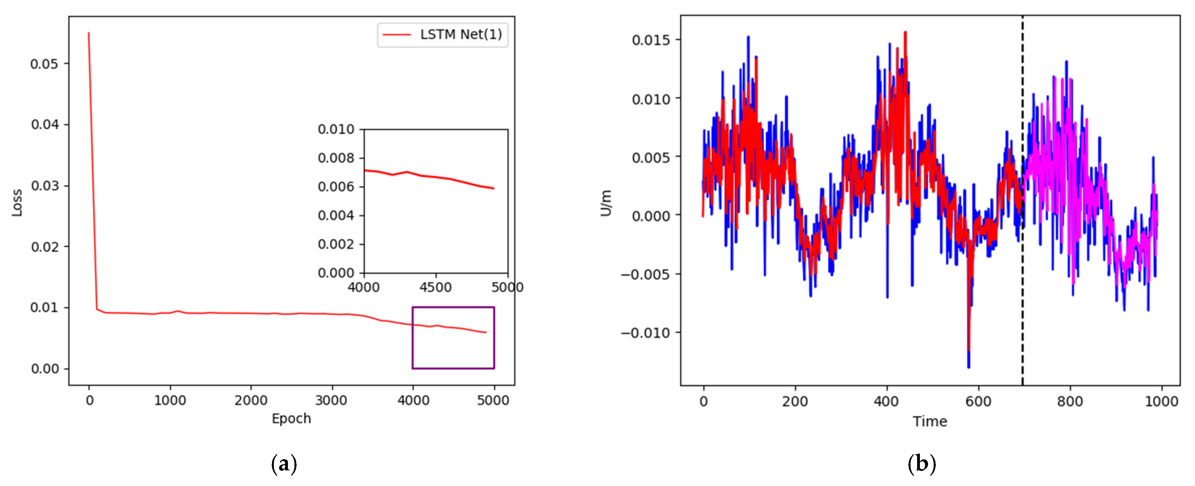
The training and prediction results of these three neural networks with different settings using different scale windows are shown in Figure 7, Figure 8 and Figure 9, respectively.

Figure 7.
(a) Training loss curve; (b) data training and prediction of XJSS using LSTM Net(1).
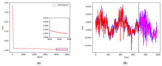
Figure 8.
(a) Training loss curve; (b) data training and prediction of XJSS using LSTM Net(2).
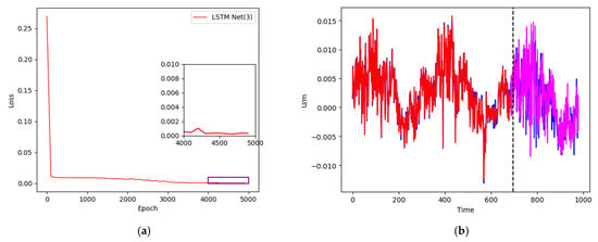
Figure 9.
(a) Training loss curve; (b) data training and prediction of XJSS using LSTM Net(3).
In the first experiment, a sliding window of 10-1 and 10 hidden cells of the single-layer LSTM were used as the network framework. The loss curve is shown in Figure 7a. We can observe that after 5000 training runs, the loss curve dropped to around 0.006. The training results and prediction results are shown in Figure 7b. The blue curve represents the original value, comprising 990 groups of data in total, the red curve denotes the training neural network, containing 696 groups of data, and the magenta curve shows the remaining 294 groups of data for prediction.
In the second experiment, a sliding window of 15-1 and 15 hidden cells of the single-layer LSTM were used as the network framework. The loss curve is shown in Figure 8a. We can observe that after 5000 training runs, the loss curve dropped to around 0.002. The training results and prediction results are shown in Figure 8b. The blue curve represents the original value, comprising a total of 985 groups of data, the red curve denotes the training neural network, containing 691 groups of data, and the magenta curve shows the remaining 294 groups of data for prediction.
In the third experiment, a sliding window of 20-1 and 20 hidden cells of the single-layer LSTM were used as the network framework. The loss curve is shown in Figure 9a. After 5000 training runs, the loss curve dropped to below 0.001. The training results and prediction results are shown in Figure 9b. The blue curve represents the original value, comprising a total of 980 groups of data, the red curve denotes the training neural network, containing 686 groups of data, and the magenta curve shows the remaining 294 groups of data for prediction.
During the training of the neural network, the lower the loss value, the better. Although a smaller loss value indicates a stronger fitting performance of the neural network to the training data, it also results in less generalization ability. In practical application, the hyperparameters can be adjusted according to the data and the neural network structure; for example, a loss value of around 0.005 can maintain a good fit and generalization ability. In addition, the use of 5000 training runs in this experiment was also based on empirical values obtained after multiple training runs.
4.2. Experiment Summary
By weighted summation of the three groups of prediction results, 294 corresponding MSSW-LSTM prediction results were obtained, as shown in the Figure 10 below.
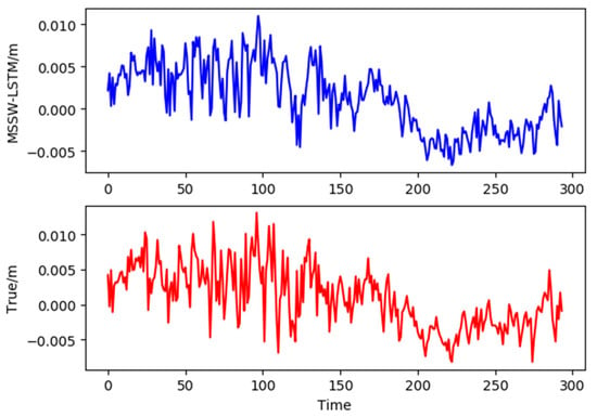
Figure 10.
Comparison of MSSW-LSTM prediction and the true values.
Figure 10 shows the comparison between the forecast results of MSSW-LSTM (blue) and the actual time series (red). It can be seen that MSSW-LSTM forecast results are consistent with the true values.
To quantitatively evaluate the prediction accuracy of our proposed model, indexes (RMSE and MAE) were used to calculate the difference between the real and predicted values. In the three LSTM experiments, the network model was obtained by training nearly 700 datapoints, and the remaining 294 datapoints were predicted. The statistical results are shown in Table 4, among which the RMSE of LSTM(1), LSTM(2), and LSTM(3) are 3.2292, 4.1424, and 3.9810, respectively, and the MAE of these three experiments are 2.4252, 3.0239, and 3.0679.

Table 4.
Performance comparison of traditional LSTM and proposed MSSW-LSTM.
We can observe that, although the network model may become more complex, the RMSE and MAE may not necessarily decrease. For example, although LSTM(2) is more complex than LSTM(1), its RMSE value is greater. It is obvious that both RMSE and MAE of MSSW-LSTM reach the best values. Specifically, RMSE is reduced by 2.1%, 23.7%, and 20.1% and MAE is decreased by 1.6%, 21.1%, and 22.2%, respectively.
In theory, through a single network, it is difficult to achieve optimal results even after multiple training runs. However, the MSSW-LSTM algorithm can combine the advantages of multiple networks and the data characteristics at different scales. The principle of this advantage is that the framework adopts the idea of measurement adjustment.
5. Discussion and Conclusions
In this study, a new forecasting framework, named MSSW-LSTM, comprising a multiscale sliding window (MSSW) and LSTM, was proposed for predicting GNSS time series. In the data preprocessing stage, the multiscale sliding window is used to form different training subsets, which can effectively extract the feature relationship under different scales, and facilitates mining the deep features of the data. The LSTM network can then effectively avoid the problem of gradient disappearance in the process of parameter solving. The MSSW-LSTM can use multiple LSTM networks to make simultaneous predictions, and obtains final results by weighting.
To verify the effectiveness of the MSSW-LSTM algorithm, 1000 daily solutions of the XJSS station in the Up component were selected for prediction experiments. The results of three groups of controlled experiments showed that the RMSE was reduced by 2.1%, 23.7%, and 20.1%, and MAE was decreased by 1.6%, 21.1%, and 22.2%, respectively. The experimental results showed that the proposed framework has a higher prediction accuracy and a smaller error.
It should be noted that the MSSW-LSTM method has significant flexibility. Researchers can easily construct appropriate subspace subsets formed by multiscale windows according to different data characteristics. In addition, LSTM networks may be the same or different, and may comprise single layer or multiple layers. This feature is beneficial to researchers for the selection of the most appropriate network model according to their own dataset characteristics, and for use of the advantages of the network model. MSSW-LSTM is a general framework for prediction that can be extended to other fields, such as traffic flow prediction, weather forecasting, and air quality forecasting.
Author Contributions
Conceptualization, J.W. and W.J.; methodology, J.W. and W.J.; software, J.W.; validation, J.W. and Z.L.; formal analysis, J.W. and Z.L.; investigation, J.W. and Y.L.; resources, J.W.; data curation, J.W.; writing—original draft preparation, J.W. and Z.L.; writing—review and editing, J.W., Z.L. and Y.L.; All authors have read and agreed to the published version of the manuscript.
Funding
This study is partially supported by the Natural Science Innovation Group Foundation of China (No. 41721003), and National key R&D Program of China (2018YFC1503601).
Institutional Review Board Statement
Not applicable.
Informed Consent Statement
Not applicable.
Data Availability Statement
Not applicable.
Acknowledgments
The authors gratefully acknowledge the China Earthquake Networks Center, National Earthquake Data Center (http://data.earthquake.cn, accessed on 16 August 2021) for providing GNSS data.
Conflicts of Interest
The authors declare no conflict of interest.
References
- Geoffrey, L.; Blewitt, D. Effect of annual signals on geodetic velocity. J. Geophys. Res. Solid Earth 2002, 107, ETG 9-1–ETG 9-11. [Google Scholar]
- Ohta, Y.; Kobayashi, T.; Tsushima, H.; Miura, S.; Hino, R.; Takasu, T.; Fujimoto, H.; Iinuma, T.; Tachibana, K.; Demachi, T.; et al. Quasi real-time fault model estimation for near-field tsunami forecasting based on RTK-GPS analysis: Application to the 2011 Tohoku-Oki earthquake (Mw 9.0). J. Geophys. Res. Solid Earth 2012, 117. [Google Scholar] [CrossRef]
- Deng, L.; Jiang, W.; Li, Z.; Chen, H.; Wang, K.H.; Ma, Y.F. Assessment of second-and third-order ionospheric effects on regional networks: Case study in China with longer CMONOC GPS coordinate time series. J. Geod. 2017, 91, 207–227. [Google Scholar] [CrossRef]
- Bevis, M.; Alsdorf, D.; Kendrick, E.; Fortes, L.P.; Forsberg, B.; Smalley, R.; Becker, J. Seasonal fluctuations in the mass of the Amazon River system and Earth’s elastic response. Geophys. Res. Lett. 2005, 32. [Google Scholar] [CrossRef] [Green Version]
- Montillet, J.P.; Williams, S.; Koulali, A.; McClusky, S.C. Estimation of offsets in GPS time-series and application to the detection of earthquake deformation in the far-field. Geophys. J. Int. 2015, 200, 1207–1221. [Google Scholar] [CrossRef] [Green Version]
- Meng, X.; Roberts, G.W.; Dodson, A.H.; Cosser, E.; Barnes, J.; Rizos, C. Impact of GPS satellite and pseudolite geometry on structural deformation monitoring: Analytical and empirical studies. J. Geod. 2004, 77, 809–822. [Google Scholar] [CrossRef]
- Yi, T.H.; Li, H.N.; Gu, M. Experimental assessment of high-rate GPS receivers for deformation monitoring of bridge. Meas. J. Int. Meas. Confed. 2013, 46, 420–432. [Google Scholar] [CrossRef]
- Yu, J.; Meng, X.; Shao, X.; Yan, B.; Yang, L. Identification of dynamic displacements and modal frequencies of a medium-span suspension bridge using multimode GNSS processing. Eng. Struct. 2014, 81, 432–443. [Google Scholar] [CrossRef]
- Xi, R.; Jiang, W.; Meng, X.; Zhou, X.; He, Q. Rapid initialization method in real-time deformation monitoring of bridges with triple-frequency BDS and GPS measurements. Adv. Space Res. 2018, 62, 976–989. [Google Scholar] [CrossRef]
- Chen, Q.; Jiang, W.; Meng, X.; Jiang, P.; Wang, K.; Xie, Y.; Ye, J. Vertical deformation monitoring of the suspension bridge tower using GNSS: A case study of the forth road bridge in the UK. Remote Sens. 2018, 10, 364. [Google Scholar] [CrossRef] [Green Version]
- Altamimi, Z.; Rebischung, P.; Métivier, L.; Collilieux, X. ITRF2014: A new release of the International Terrestrial Reference Frame modeling nonlinear station motions. J. Geophys. Res. Solid Earth 2016, 121, 6109–6131. [Google Scholar] [CrossRef] [Green Version]
- Li, Z.; Chen, W.; van Dam, T.; Rebischung, P.; Altamimi, Z. Comparative analysis of different atmospheric surface pressure models and their impacts on daily ITRF2014 GNSS residual time series. J. Geod. 2020, 94, 1–20. [Google Scholar] [CrossRef]
- Zhang, J.; Bock, Y.; Johnson, H.; Fang, P.; Williams, S.; Genrich, J.; Wdowinski, S.; Behr, J. Southern California permanent GPS geodetic array: Error analysis of daily position estimates and site velocities. J. Geophys. Res. Solid Earth 1997, 102, 18035–18055. [Google Scholar] [CrossRef]
- He, X.; Montillet, J.P.; Fernandes, R.; Bos, M.; Yu, K.; Hua, X.; Jiang, W. Review of current GPS methodologies for producing accurate time series and their error sources. J. Geodyn. 2017, 106, 12–29. [Google Scholar] [CrossRef]
- Klos, A.; Olivares, G.; Teferle, F.N.; Hunegnaw, A.; Bogusz, J. On the combined effect of periodic signals and colored noise on velocity uncertainties. GPS Solut. 2018, 22, 1–13. [Google Scholar] [CrossRef] [Green Version]
- Hinton, G.E.; Salakhutdinov, R.R. Reducing the Dimensionality of Data with Neural Networks. Science 2006, 313, 504–507. [Google Scholar] [CrossRef] [Green Version]
- Rumelhart, D.E.; Hinton, G.E.; Williams, R.J. Learning representations by back-propagating errors. Nature 1986, 323, 533–536. [Google Scholar] [CrossRef]
- Elman, J.L. Finding structure in time. Cogn. Sci. 1990, 14, 179–211. [Google Scholar] [CrossRef]
- Bengio, Y.; Simard, P.; Frasconi, P. Learning long-term dependencies with gradient descent is difficult. IEEE Trans. Neural Netw. 1994, 5, 157–166. [Google Scholar] [CrossRef]
- Hochreiter, S.; Schmidhuber, J. Long short-term memory. Neural Comput. 1997, 9, 1735–1780. [Google Scholar] [CrossRef]
- Freeman, B.S.; Taylor, G.; Gharabaghi, B.; Thé, J. Forecasting air quality time series using deep learning. J. Air Waste Manag. Assoc. 2018, 68, 866–886. [Google Scholar] [CrossRef]
- Karevan, Z.; Suykens, J. Transductive LSTM for time-series prediction: An application to weather forecasting. Neural Netw. 2020, 125, 1–9. [Google Scholar] [CrossRef]
- Tian, Y.; Pan, L. Predicting short-term traffic flow by long shortterm memory recurrent neural network. In Proceedings of the 2015 IEEE International Conference on Smart City/SocialCom/SustainCom (SmartCity), Chengdu, China, 19–21 December 2015; IEEE: Piscataway, NJ, USA, 2015; pp. 153–158. [Google Scholar]
- Xing, Y.; Yue, J.; Chen, C.; Cong, K.L.; Zhu, S.L.; Bian, Y.K. Dynamic Displacement Forecasting of Dashuitian Landslide in China Using Variational Mode Decomposition and Stack Long Short-Term Memory Network. Appl. Sci. 2019, 9, 2951. [Google Scholar] [CrossRef] [Green Version]
- Xing, Y.; Yue, J.; Chen, C. Interval Estimation of Landslide Displacement Prediction Based on Time Series Decomposition and Long Short-Term Memory Network. IEEE Access 2020, 8, 3187–3196. [Google Scholar] [CrossRef]
- Xie, P.; Zhou, A.; Chai, B. The Application of Long Short-Term Memory(LSTM) Method on Displacement Prediction of Multifactor-Induced Landslides. IEEE Access 2019, 7, 54305–54311. [Google Scholar] [CrossRef]
- Wang, J.; Nie, G.; Gao, S.; Wu, S.; Li, H.; Ren, X. Landslide Deformation Prediction Based on a GNSS Time Series Analysis and Recurrent Neural Network Model. Remote Sens. 2021, 13, 1055. [Google Scholar] [CrossRef]
- Yang, B.; Yin, K.; Lacasse, S.; Liu, Z.Q. Time series analysis and long short-term memory neural network to predict landslide displacement. Landslides 2019, 16, 677–694. [Google Scholar] [CrossRef]
- Tan, T.N.; Khenchaf, A.; Comblet, F.; Franck, P.; Champeyroux, J.M.; Reichert, O. Robust-Extended Kalman Filter and Long Short-Term Memory Combination to Enhance the Quality of Single Point Positioning. Appl. Sci. 2020, 10, 4335. [Google Scholar] [CrossRef]
- Jiang, C.; Chen, S.; Chen, Y.; Zhang, B.; Feng, Z.; Zhou, H.; Bo, Y. A MEMS IMU De-Noising Method Using Long Short Term Memory Recurrent Neural Networks (LSTM-RNN). Sensors 2018, 18, 3470. [Google Scholar] [CrossRef] [Green Version]
- Kim, H.U.; Bae, T.S. Deep Learning-Based GNSS Network-Based Real-Time Kinematic Improvement for Autonomous Ground Vehicle Navigation. J. Sens. 2019, 2019, 1–8. [Google Scholar] [CrossRef]
- Tao, Y.; Liu, C.; Chen, T.; Zhao, X.W.; Liu, C.Y.; Hu, H.J.; Zhou, T.F.; Xin, H.Q. Real-Time Multipath Mitigation in Multi-GNSS Short Baseline Positioning via CNN-LSTM Method. Math. Probl. Eng. 2021, 2021, 1–12. [Google Scholar]
- Hoang, M.T.; Yuen, B.; Dong, X.; Lu, T.; Westendorp, R.; Reddy, K. Recurrent Neural Networks for Accurate RSSI Indoor Localization. IEEE Internet Things J. 2019, 6, 10639–10651. [Google Scholar] [CrossRef] [Green Version]
- Fang, W.; Jiang, J.; Lu, S.; Gong, Y.; Tao, Y.; Tang, Y.; Yang, P.; Luo, H.; Liu, J. A LSTM Algorithm Estimating Pseudo Measurements for Aiding INS during GNSS Signal Outages. Remote Sens. 2020, 12, 256. [Google Scholar] [CrossRef] [Green Version]
- Redmon, J.; Farhadi, A. YOLO9000: Better, Faster, Stronger. In Proceedings of the IEEE Conference on Computer Vision & Pattern Recognition, Honolulu, HI, USA, 21–26 July 2017; pp. 6517–6525. [Google Scholar]
- Ren, S.; He, K.; Girshick, R.; Girshick, R.; Sun, J. Faster R-CNN: Towards Real-Time Object Detection with Region Proposal Networks. IEEE Trans. Pattern Anal. Mach. Intell. 2017, 39, 1137–1149. [Google Scholar] [CrossRef] [Green Version]
- Plutowski, M.; Cottrell, G.; White, H. Experience with selecting exemplars from clean data. Neural Netw. Off. J. Int. Neural Netw. Soc. 1996, 9, 273–294. [Google Scholar] [CrossRef]
Publisher’s Note: MDPI stays neutral with regard to jurisdictional claims in published maps and institutional affiliations. |
© 2021 by the authors. Licensee MDPI, Basel, Switzerland. This article is an open access article distributed under the terms and conditions of the Creative Commons Attribution (CC BY) license (https://creativecommons.org/licenses/by/4.0/).


