Abstract
Synthetic aperture radar (SAR) acquisitions are mainly deemed suitable for mapping dynamic land-cover and land-use scenarios due to their timeliness and reliability. This particularly applies to Sentinel-1 imagery. Nevertheless, the accurate mapping of regions characterized by a mixture of crops and grasses can still represent a challenge. Radar time-series have to date mainly been exploited through backscatter intensities, whereas only fewer contributions have focused on analyzing the potential of interferometric information, intuitively enhanced by the short revisit. In this paper, we evaluate, as primary objective, the added value of short-temporal baseline coherences over a complex agricultural area in the São Paulo state, cultivated with heterogeneously (asynchronously) managed annual crops, grasses for pasture and sugarcane plantations. We also investigated the sensitivity of the radar information to the classification methods as well as to the data preparation and sampling practices. Two supervised machine learning methods—namely support vector machine (SVM) and random forest (RF)—were applied to the Sentinel-1 time-series at the pixel and field levels. The results highlight that an improvement of 10 percentage points (p.p.) in the classification accuracy can be achieved by using the coherence in addition to the backscatter intensity and by combining co-polarized (VV) and cross-polarized (VH) information. It is shown that the largest contribution in class discrimination is brought during winter, when dry vegetation and bare soils can be expected. One of the added values of coherence was indeed identified in the enhanced sensitivity to harvest events in a small but significant number of cases.
1. Introduction
Space-borne radar sensors are deemed to play an important role in agriculture and land cover monitoring, mainly due to their potential to provide images independently of the weather and solar illumination conditions, but also for their complementary sensitivity to physical retrievables with respect to optical sensors. The use of SAR data to discriminate different land cover types was already demonstrated using ERS-1/2 data [1,2]. The Sentinel-1 mission [3] provided, for the first time, dense systematic time-series of radar scattering and interferometric coherences in C-Band and dual-polarization (VV and VH) with a repeat-sampling interval of 6 or 12 days. Its interferometric wide (IW) swath mode provides data with swath widths of approximately 250 at 5 by 20 single-look spatial resolution.
Land use/land cover (LULC) mapping using SAR data is commonly implemented using data-driven methods [4,5,6,7] which do not require the statistical modeling of the land cover signatures and of their patterns in time, often characterized by significant complexities. Data-driven methods, such as random forest (RF), support vector machine (SVM) and neural network classifiers, can account for underlying relationships between features in dense data series in a cost- and performance-effective way. Dense time series are known to be the key for reliable mapping as they enable the exploitation of the dissimilarities in the signature of different LULC classes during specific days of the year, particularly useful for vegetated classes with dynamic phenology such as crops [8].
Most of the land cover mapping studies exploit SAR intensity. However, the complex-valued correlation coefficients between SAR images, i.e., the interferometric coherence, also provide information about the land cover classes’ characteristics [9]. The time-series of coherence images can provide information about events, such as mowing events [10,11], which can serve as the smoking gun that distinguishes one LULC type from another.
Considering InSAR information as an input feature for land cover classification is not a new concept. Previous studies have already confirmed the potential of InSAR coherence for LULC classification, e.g., using time-series of ERS data with a one day revisit time [1,12] and a stack of 12 days of Sentinel-1 images [13]. Single-pass interferometric coherence acquired by TanDEM-X and repeat-pass coherence from the TerraSAR-X mission was employed for crop-type mapping in [14,15], respectively. Furthermore, in [9], the authors showed that the temporal dynamics and spatial context of the multi-temporal InSAR coherence can enhance the performance of land cover classification.
In addition, the study by [16] utilized backscattering with estimated parameters from a temporal decorrelation model as input features for large scale land cover mapping over short-time-series of Sentinel-1 images. The study by [6] presented the LULC classification map by applying SVM and RF on different combinations of Sentinel-1 attributes including backscattering, interferometric coherence and polarimetric H- decomposition attributes of two single look complex (SLC) images. It showed that the best performance was achieved by providing all the available features to an RF classifier. Moreover, mean backscatter, backscatter difference and the coherence information of two SLC Sentinel-1 images were employed to separate the water, barren, vegetation and built-up classes through maximum likelihood classification [17]. However, despite the noteworthy efforts, the benefits of using the coherence time-series for LULC mapping have not been fully understood and exploited yet. The identification of the physical events, highlighted by the coherence, which help in discriminating between different land cover types, still represents an open investigation area.
The objective of the paper is then to shed further light on the added value of coherence, when combined with the backscattered intensities, for mapping naturally vegetated and cultivated areas with dual-polarized (VV and VH) Sentinel-1 data time-series. The use of coherence information heavily increases the numbers of features in the classification problem. Whereas only one value per acquisition shall be considered for amplitudes, and therefore a total of N values for N acquisitions, the number of image pairs that can be potentially addressed for coherence features is . However, since previous efforts [13] showed that most of the sensitive information is carried in short-term coherences, only consecutive acquisitions will be used to estimate the cross-correlation between SAR images. The objective of the paper is to evaluate the added value of coherence in SAR-based land cover mapping. Our aim was then to identify which kind of exploitable information, complementary to the VH and VV amplitude, the coherence can provide. Coherences are typically low, which leads to significant uncertainties in their estimates. Therefore, we also explore and compare two different approaches to estimate the coherences: one based on a standard fixed-resolution multi-looking approach, and one taking advantage of contextual information by averaging per field.
2. Study Area and Data
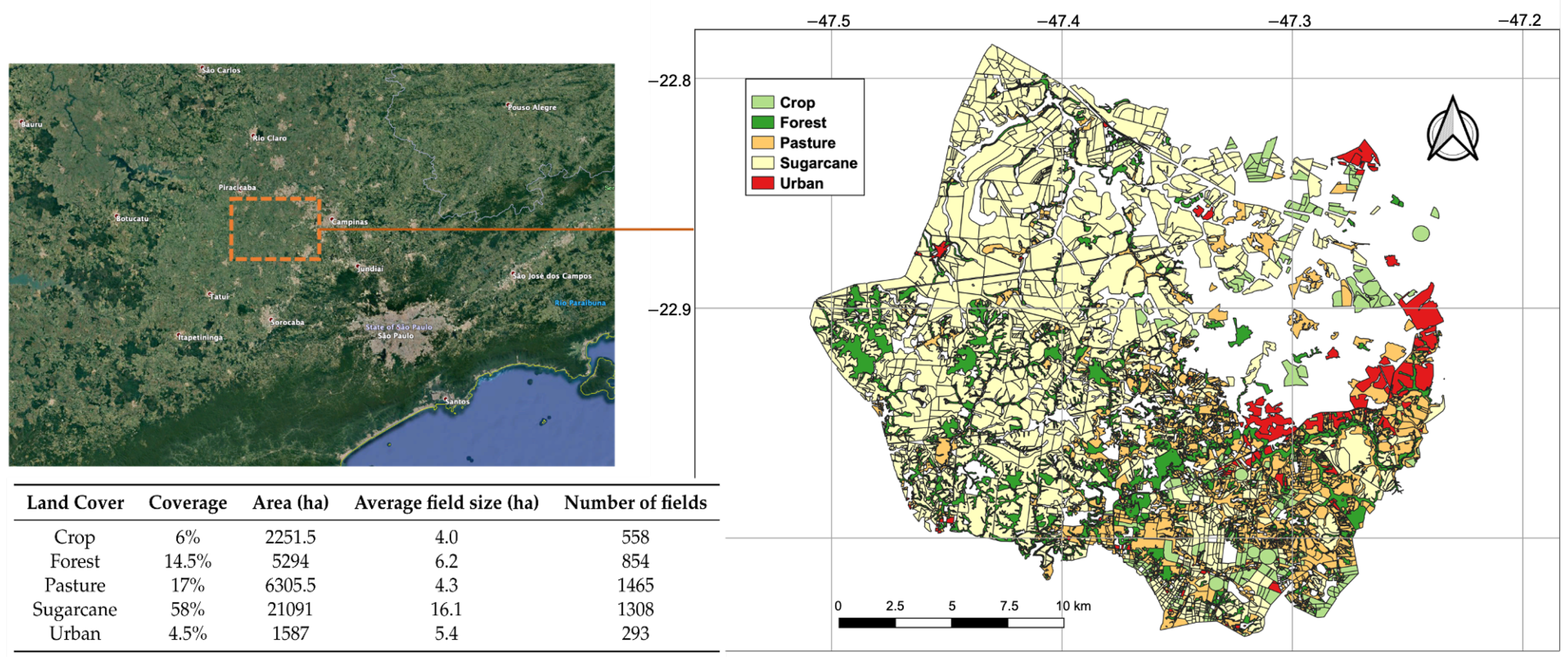
The study area is situated near Campinas in the São Paulo state, Brazil. São Paulo has a tropical and subtropical climate with long and hot summers. The mean temperature reaches 30 C in the warmest months with heavy rainfall. Conversely, the winter months are mostly dry. The vegetation shows lower biomass and also lower greenness due to these seasonality changes. Crop and pasture fields are commonly rain-fed. Irrigation can be occasionally applied to annual crops at the beginning of the growth cycle [18]. The reference dataset consists of the LULC information collected both from ground surveying activities in 2015 and from the visual inspection and interpretation of 2016–2017 high resolution optical imagery such as Google Earth imagery, Landsat and MODIS time series, manually digitized into polygons. The fields are grouped into five LULC classes/categories: crop, forest, pasture, sugarcane and urban. The crop class includes mostly soybean, wheat and corn. The forest class contains native and production forests. Pasture fields, used for cattle grazing, and sugarcane, with a crop cycle of 12–18 months, expand over grasslands [19]. As conveyed by Table 1, the sugarcane cycle typically starts between September and November, whereas annual crops are characterized by two different emerging periods throughout the year, in spring (April–June) and in autumn (November–December), and can be subject to double cropping practices. The spatial map of the reference LULC and some of the polygons’ characteristics, arranged per class, are shown in Figure 1.

Table 1.
Distribution of the start of growth dates throughout the year (percentages are reported) for annual crops and sugarcane fields.
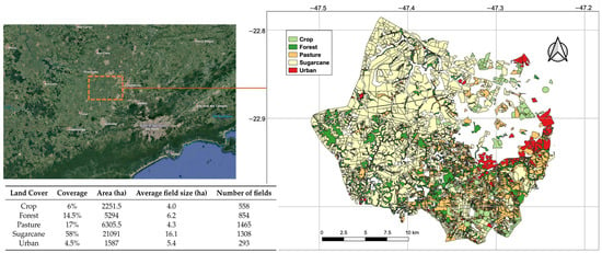
Figure 1.
Location of the study area (top left); spatial map of the reference LULC (right); and characteristics of the LULC based on the collected ground truth data (bottom left).
A total of 28 available Sentinel-1 (S1) Interferometric Wide (IW) acquisitions were employed, covering one year between November 2016 and October 2017. Since only one satellite (Sentinel-1B) is active in IW mode over this region, the revisit time is 12 days. The study area is illuminated with an average incidence angle of 35. The sensor has a resolution of 20 (in the azimuth direction) × (in the ground range direction). As a result, approximately 4.5 looks are available in a m cell and 110 over a m cell. Although the classification is only performed by using radar features, the normalized difference vegetation index (NDVI) from Landsat-8 data is also employed in this study for the visual interpretation of the Sentinel-1 behavior. The NDVI index expresses the greenness of canopies and can hence be readily related to crop cycles and plant status throughout the seasons. According to [20,21], the NDVI can be affected by topography but in our study, for visual inspection purposes, the impact of this variable can be considered negligible. The Landsat-8 surface reflectance products, provided by USGS, have been retrieved using the Google Earth Engine (GEE). Only Landsat products with less than 40% of the total tile area covered by clouds were used in order to ensure that the collected NDVI series is only negligibly affected by atmospheric effects. Although it will not include all the cloud-free acquisitions, such an arbitrary choice is deemed a convenient compromise for our visual interpretation purposes.
3. Methods
3.1. Pre-Processing
The S1 IW acquisitions are downloaded in their SLC product format from the ESA hub. The data processing is performed using the Radar Interferometric Parallel Processing Lab (RIPPL), a TU Delft’s in-house Sentinel-1 InSAR processing tool. Figure 2 provides an overview of the processing steps performed to obtain the interferometric coherences. Only the interferograms between the consecutive (12-days interval) image pairs are formed and subsequently geo-referenced. The backscatter intensity computation includes the radiometric calibration and terrain correction steps. SRTM-3 [22] is used as an external digital elevation model (DEM) for processing. For both backscatter and coherences, two types of outputs are produced by the final spatial averaging step: one by using the conventional boxcar filter for spatial multi-looking (for the pixel-based classification); and the other by averaging within the reference polygons (for object/polygon-based classification) addressed in Section 3.3. For the pixel-based approach, three filter sizes, i.e., 40, 100 and 200 m, were tested in order to evaluate the most convenient trade-off between the radiometric quality (as a reference, 100 independent looks would lead to a precision of approximately 0.5 dB) and the mixed field effects (most of the fields are larger than 2–3 ha, as can be seen in Figure 1).
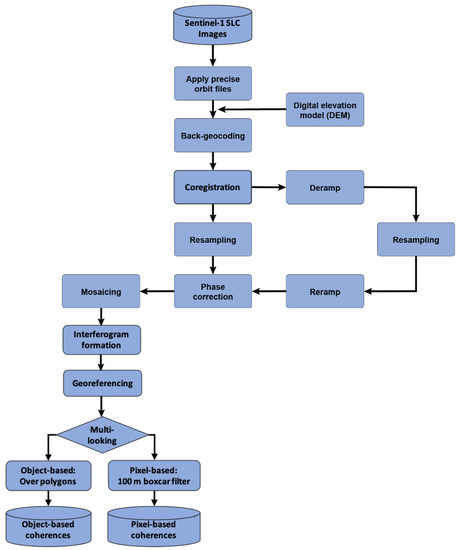
Figure 2.
Processing chain for coherence feature extraction from the SLC Sentinel-1 images.
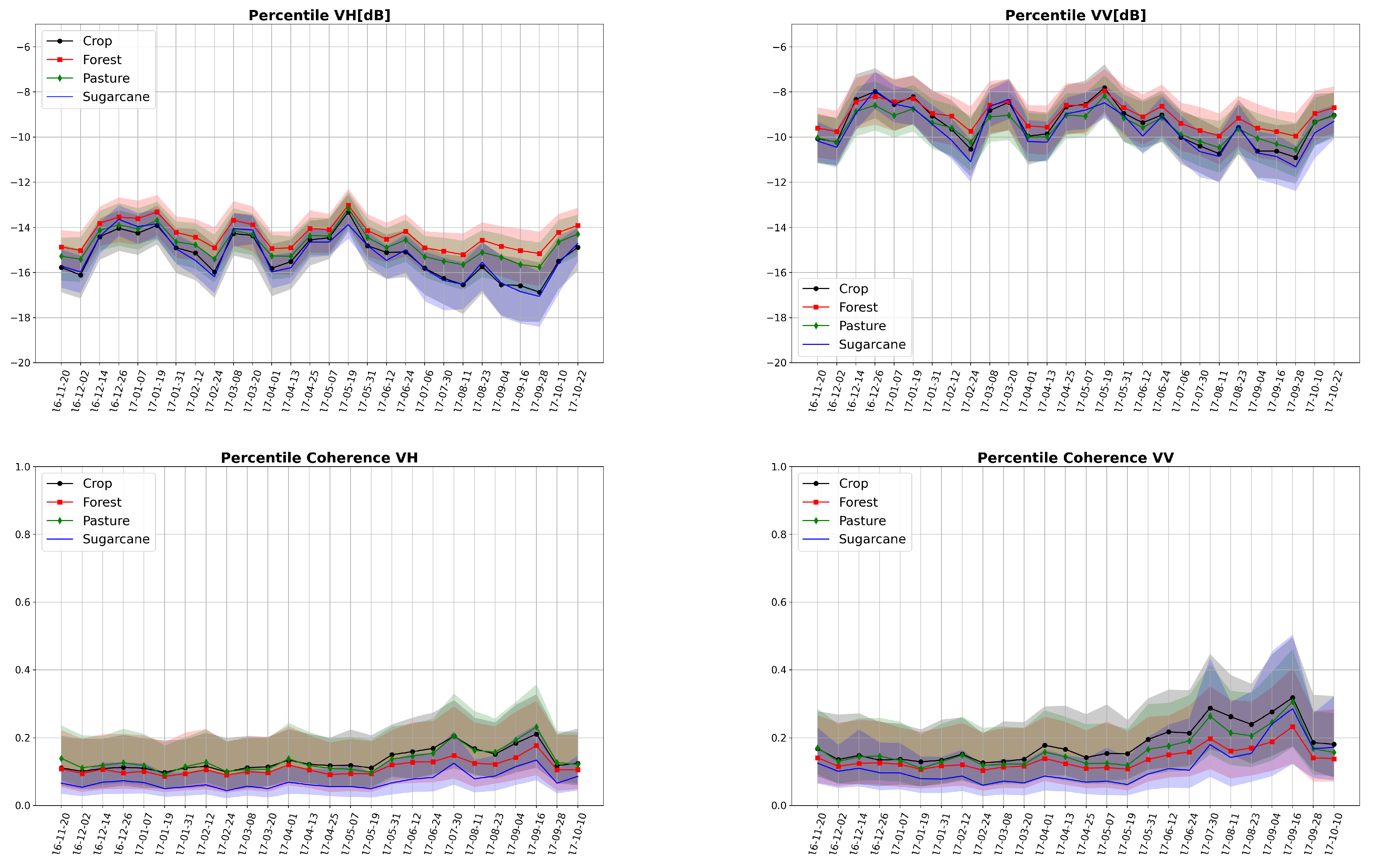
Figure 3 shows the temporal signatures of the coherence and backscatter intensity for the vegetation classes extracted from the object-based features. The statistics strongly convey the need for multi-temporal classification as the distance between the classes, evaluated on single features per epoch, is insufficient. This is particularly true for the coherence that presents inter-class dynamics only at the end of the dry season (June–September).
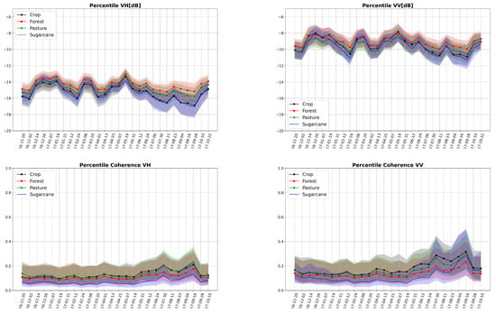
Figure 3.
Temporal statistics of the backscatter intensity (top) and coherence (bottom) for the vegetation classes. The 50th percentiles (solid lines) and the 20th–80th percentiles (transparent buffer) are based on the features derived from the field sampling approach.
3.2. Interferometric Coherence
The interferometric coherence, which is commonly used as an indicator of the quality of the interferometric phase, is defined as the normalized cross-correlation between two coregistered SAR images. The absolute value of the coherence varies between 0 and 1. In this paper, for each new image, the coherence is computed with respect to the previous image. The coherence measures the relative stability of the scattering mechanisms within a spatial neighborhood between a pair of images. If all the backscattering elements maintain their relative position and scattering strength during the 12-day time-interval, the coherence will be high. This is typically the case for bare soil and urban areas. In contrast, if the elements move or alter their microwave signature, a low value of coherence will be the outcome. This typically occurs for vegetated surfaces with high fractional canopy cover and for water. The interferometric coherence is defined as
where and represent two coregistered complex images, represents the mathematical expectation, and denotes the complex conjugate operator. Following common practice in the InSAR literature (e.g., [23]), the coherence is estimated by replacing the expectation operator by a sampled average over a given spatial window. This assumes that the signal is ergodic and locally homogeneous:
The average number of samples and the coherence map resolution have a significant impact on the coherence magnitude estimate accuracy [24]. The estimated coherence is typically noisy with a large estimation uncertainty, particularly for the small averaging windows and low coherence values.
It is worth noting that computing space-averaged coherence magnitude over entire fields improves the estimation of the coherence as the number of averaged samples increases and the quality of the estimator now depends on the field extent. Specifically, under the assumption of homogeneity, larger fields have higher coherence estimation precision and lower bias, while the smaller fields provide more bias [25]. The bias of the coherence for a homogeneous area is given by [26]
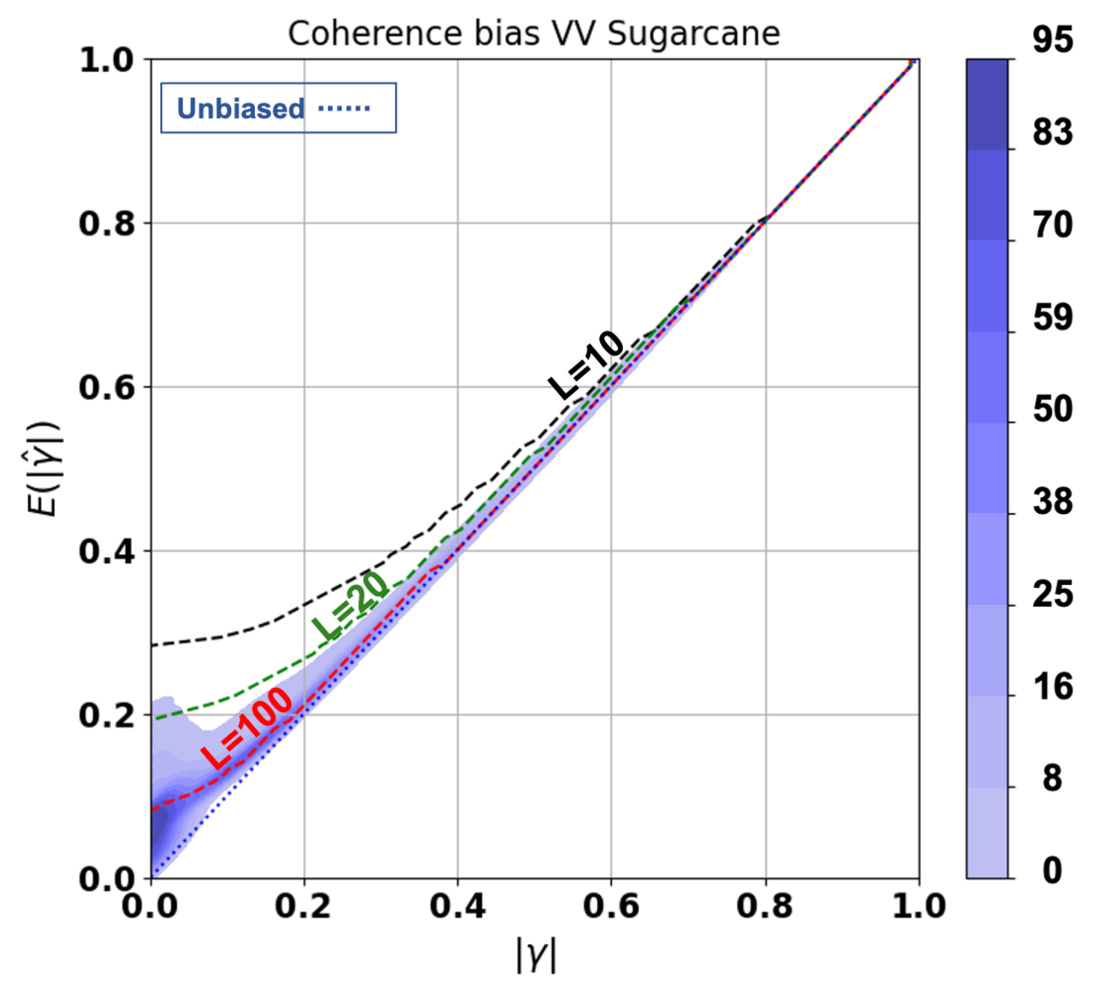
where is the hypergeometric function and L is the number of independent samples. Figure 4 shows the coherence magnitude estimate as a function of coherence magnitude () for the number of pixels for each sugarcane field used in this study.

Figure 4.
Coherence magnitude bias of sugarcane fields with different number of samples L. The color refers to the number of fields.
We can see that the coherence magnitude estimate is positively biased, especially for low coherences. Bias and/or coherence estimation uncertainty reduces for fields with more independent samples.
3.3. Land Cover Classification
In this study, the supervised classifications are performed at a pixel- and object-level. The pixel-based approach has a clear advantage in terms of implementation, as no further processing steps in addition to the spatial multi-looking in the earlier data preparation stages is required. In the most common case, a moving average filter with the desired spatial support is used for both amplitude and coherence. The major drawback of pixel-based approaches is that the spatial context of the scene is not fully exploited [27,28]. This aspect would be particularly relevant over distributed scatterers, due to their intrinsic noisy nature. Identifying homogeneous segments, i.e., groups of pixels that share similar land cover, in order to average as many looks as possible, naturally leads to the so-called object-based classification.
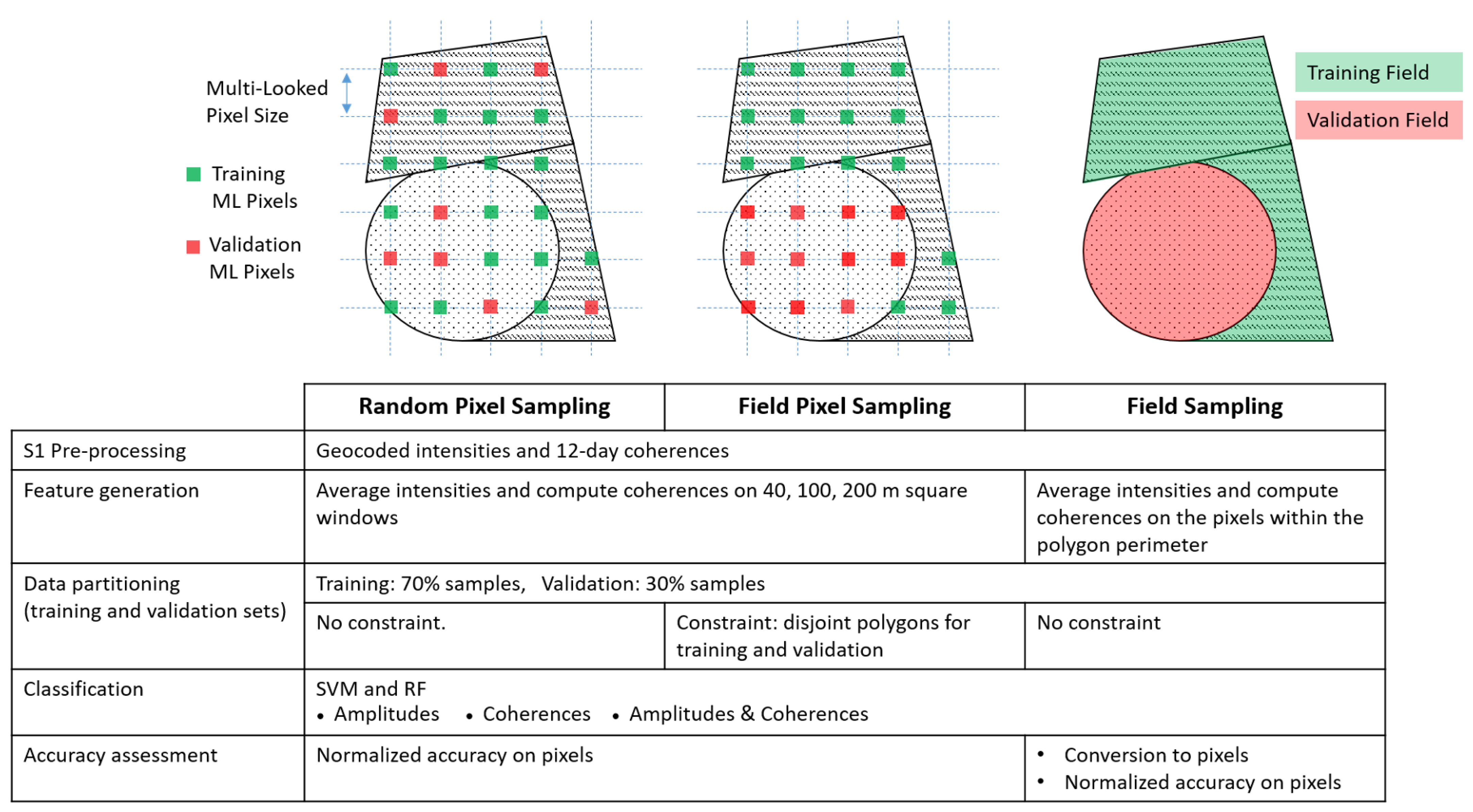
We consider three schemes to generate training and validation sub-sets, the first two associated to the pixel-based approach and the third to the object-based approach. A visual representation of these schemes is provided in Figure 5. For all three schemes, a common cross-validation procedure is used to avoid positively biased results. Algorithms are therefore trained with 70% of the dataset, while the remaining 30% is used for validation. More specifically, the three addressed strategies are:

Figure 5.
(Top) Sketched illustration of the pixel-based and field-based sampling schemes for three polygons belonging to the same class. The different patterns in the polygon background represent intra-class diversity; (Bottom) For each sampling scheme, the methodology steps from image pre-processing to accuracy evaluation are briefly summarized.
- Random-Pixel Sampling: The pixel samples are randomly assigned to the training and validation sets without any spatial context constraint. The outcome is that any arbitrary field is allowed to have part of its pixels in the training set and part in the validation set. This is expected to lead to a positive bias in accuracy due to eventual overfitting, which occurs when the intra-polygon variability is lower than the variability between polygons of the same class. The risk in this random sampling approach is therefore that the algorithm learns the behavior of the individual fields rather than modeling their common statistical traits.
- Field-Pixel Sampling: In this approach, the pixels from the same polygon are entirely assigned either to the training or the validation set. For each class, the training set is built by iterative growth, i.e., by adding a field at a time to the set until 70% of the total pixels are allocated. The pixels from the excluded fields are assigned to the validation set.
- Field Sampling: This refers to object-based classification, as the samples correspond to the polygons themselves. The coherence magnitude and the backscatter intensity features are computed through multi-looking over the entire field. The differences with the field-pixels sampling are found in the impact of intra-field heterogeneities and in the different sensitivity to speckle noise. We are using the digitalized polygons (or objects or segments) from our ground surveying activities.
For each of these schemes, SVM [29] and RF [30] supervised classification are individually tested on the intensity and on the coherence stacks and then applied to the combination of the intensity and coherence in the two polarizations. The classification methods are implemented in Python using the scikit-learn package [31]. With concern to the SVM, the radius basis function (RBF) kernel [32] has been used. Two important parameters for the RBF kernel must be considered: the trade-off between margin and misclassification (C) and the kernel width () that controls the influence of the feature data point on the decision boundary. In our study, SVM was run with C = 1 and . As regards the RF, the algorithm was applied by adopting a number of trees (Ntree) equal to 100 and default values for the other parameters.
The accuracy assessment was carried out by analyzing the overall accuracy, the kappa index, and the producer’s and user’s accuracies [33]. The producer’s accuracy is related to the omission error and is defined as the number of correctly classified samples divided by the total number of reference samples in the given class. The user’s accuracy instead represents the commission error and is defined as the number of correctly classified samples divided by the total number of classified samples in the given class. Such well-known metrics are computed after normalizing the confusion matrix by the number of samples for each class, therefore forcing an equivalent true area for all the classes. The rationale is to prevent the accuracy being dominated by the classes with larger coverage.
To fairly compare the results of the field sampling with the two pixel sampling strategies, we consider the statistics based on the number of pixels, i.e., considering the classified area. As a result, larger objects have more weight than smaller ones in the validation but not in the training part. This represents a reasonable evaluation practice, provided that the objective of the mapping application is to minimize the misclassified area rather than the number of objects. The steps of the methodology so far discussed are summarized in Figure 5.
3.4. Feature Relevance
In order to assess the set of available features, we carried out a feature relevance analysis. This can help in identifying the physical processes that make a given feature useful, and lead to more robust or more optimal classification strategies. Feature relevance can be evaluated using different metrics such as the correlation between the feature and the target variable (class membership), mutual information or information gain. These metrics are independent of the classification algorithm used [34]. The most common feature selection methods are based on mutual information. However, often they do not address the correlation between features that causes feature redundancy. In this paper, we adopted the minimum-redundancy–maximum-relevance (mRMR) algorithm The algorithm searches for the subset of features (S), containing n features , that maximizes the dependency (D) of the feature set on the target class through the mean value of the mutual information:
where c is the target class and is the size (number of elements) of S. I is the mutual information, defined by
with being the joint probability density function (PDF) of the two variables and and standing for the corresponding marginal PDFs.
Merely maximizing D is likely to result in sets of features that are highly correlated. This redundancy can be quantified using the mean mutual information between the features within the set:
which should be minimized. The mRMR algorithm combines the two mentioned constraints [35,36] by maximizing .
4. Results and Discussion
4.1. Quantitative Accuracy
The impact on the SAR classification performance of the three factors of interest, i.e., the sampling scheme (random pixel, field pixel, field), the classification method (SVM and RF) and the radar feature set (amplitude, coherences and their combination) is herein analyzed. The overall accuracies (OA) and kappa indices for the most effective configurations in terms of performance are presented in Table 2. It can be observed that the SVM classification approach has better performance than the RF method. In the SVM case with random-pixel sampling, when the amplitude of only one polarization is given as an input to the classifier, the overall accuracy (OA) and kappa coefficient are approximately 60% and 0.50, respectively, for both VV and VH. When using both polarization intensities, the algorithm has an improvement of roughly 8 p.p., reaching 68% OA. The VV and VH coherences, , , add a further 2 p.p. enhancement to the overall accuracy, and a 0.03 increase in the kappa coefficient. A similar behavior is also observed in the RF case with random-pixel sampling, although with lower accuracies.

Table 2.
The calculated overall accuracy and kappa coefficient for different features with SVM and RF.
In the field-pixel sampling configurations, the accuracies are lower compared to the random-pixel sampling for both classifiers. This is indeed in line with our expectations. Such an approach is nevertheless deemed more reliable, since the chances of model overfitting are lower. In the field sampling approach, i.e., using averages based on polygons instead of averages based on pixels, the accuracy of SVM experiences a 7 p.p. increase when compared to the field-pixel approach. Still with reference to Table 2, we observe that the incorporation of the coherences leads to a statistically significant improvement in accuracy in all configurations. The added value of the coherence in crop mapping was also registered by TanDEM-X data covering a shorter time interval (three months), in [14], and by Sentinel-1 time-series covering a different agricultural environment in [37].
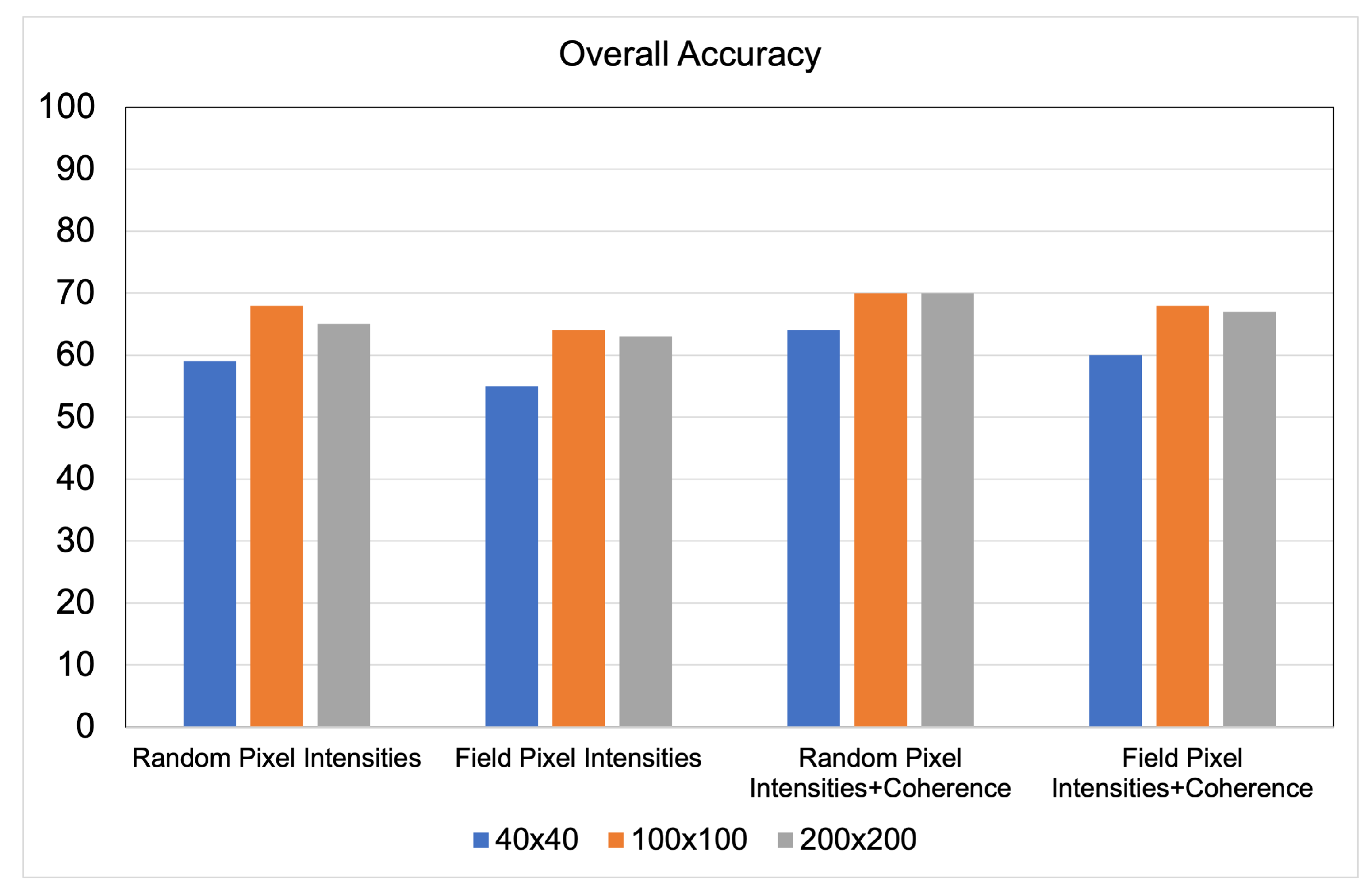
As mentioned in Section 3.1, the impact of the multi-looking window size for the pixel-based approaches was evaluated. The overall accuracy achieved by the three window sizes (40 × 40 m, 100 × 100 m and 200 × 200 m) with the SVM classifier is compared in Figure 6. The figure shows that when 40 × 40 m windows are used, the accuracies are low due to speckle noise. The accuracies for the 200 × 200 m windows are then lower compared to the 100 × 100 m configuration due to an increased amount of mixed pixel, i.e., pixels that cover two or more neighboring fields.
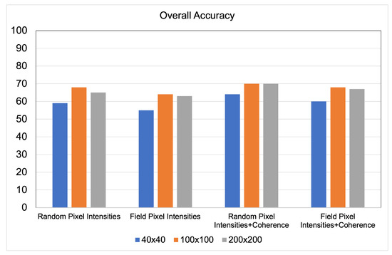
Figure 6.
The comparison between the impact of the different multi-looking window sizes on overall accuracy achieved by SVM in pixel sampling.
Although the overall accuracy gives a general understanding of a classifier’s performance, it does not reveal any information about the error partition among the classes, e.g., whether some land covers are identified more correctly than others. Confusion matrices, producer and user accuracy are then used to provide more insight. As SVM performed better than RF, in the following, only the results of SVM are presented.
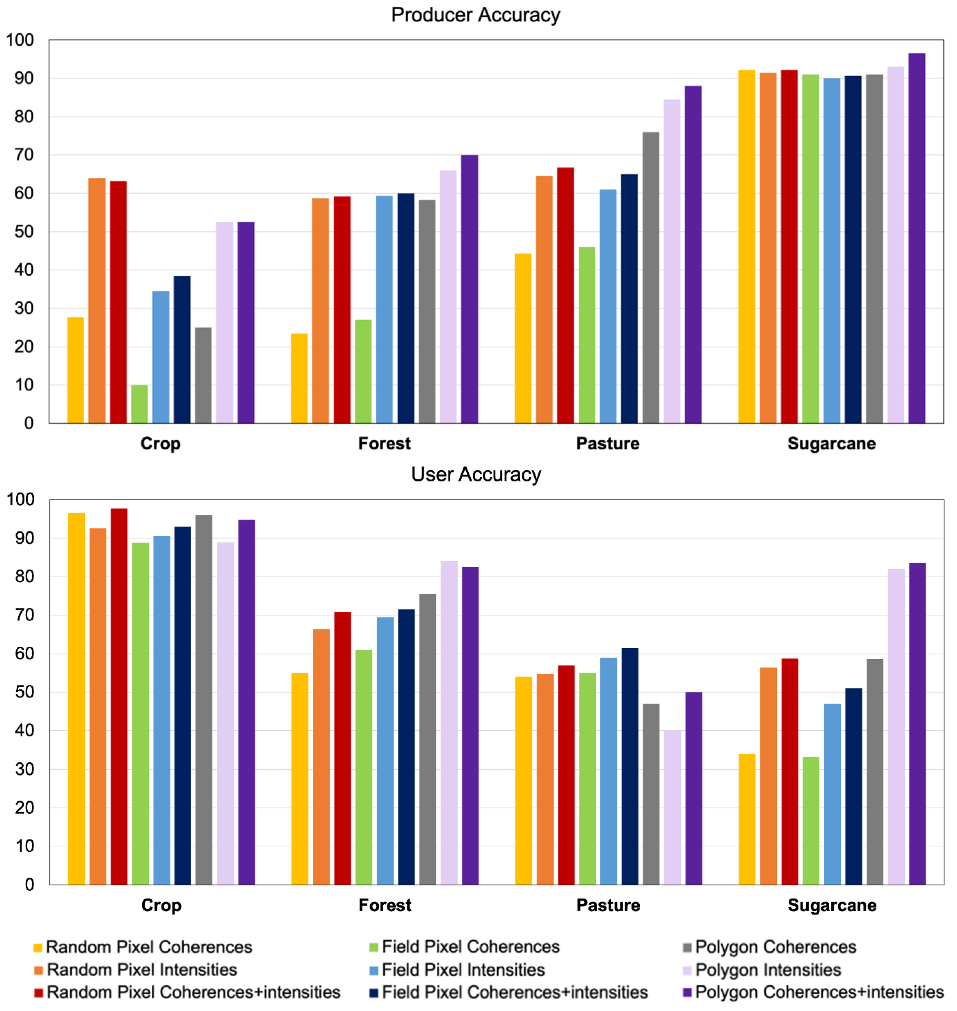
From the producer and user accuracies, as shown in Figure 7, it is straightforward to notice that the intensities perform significantly better than the coherences. By looking at their combination, it can be seen, however, that the coherence has added value for each land cover class. The largest benefits are registered by the polygon-based classification, with a fundamental 6–10 p.p. user accuracy increment for the crop and pasture classes, that are the lowest scoring classes in absolute terms.
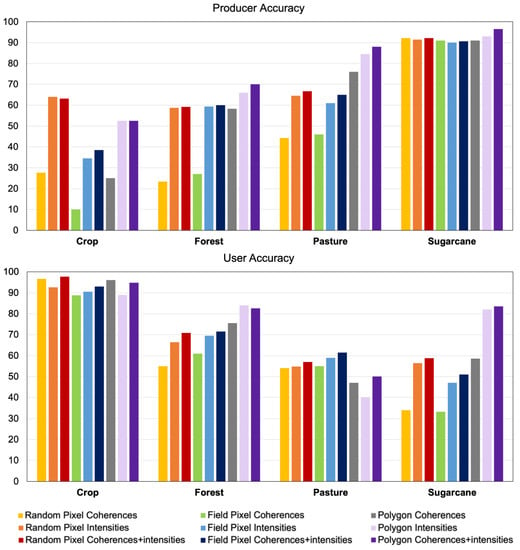
Figure 7.
Producer (top) and user (bottom) accuracy achieved by the SVM classification for different sampling schemes and feature configurations.
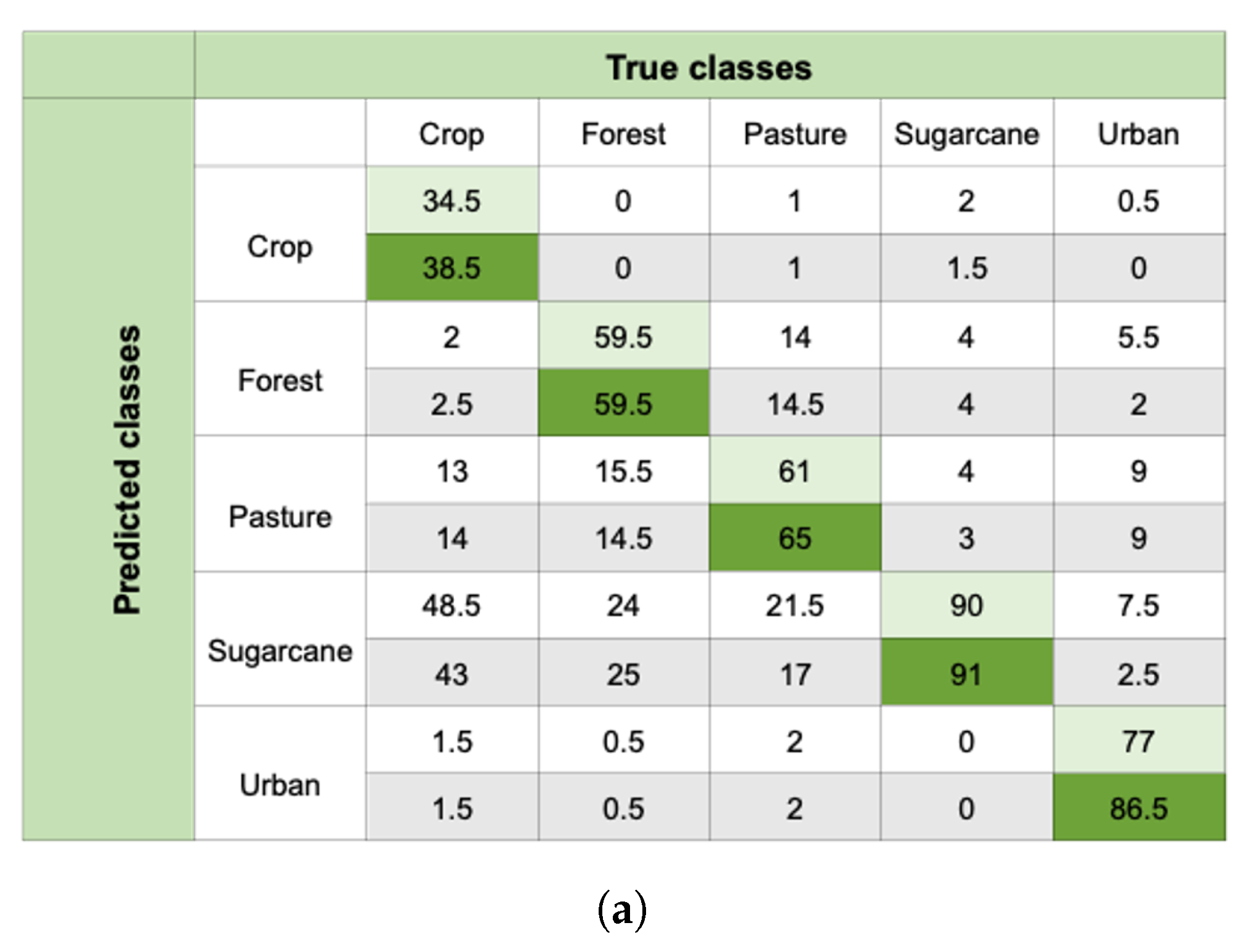
The confusion matrices, as shown in Figure 8, provide a more detailed picture, also including the urban/built-in class. In each cell, the upper value (light green) corresponds to the results obtained using only the backscattered intensities, while the lower value (dark green) corresponds to the joint use of intensities and coherences. As already specified in Section 3.3, the columns were normalized by the number of samples of the corresponding class. With such a setting, the diagonal cells contain the producer accuracy. As expected, the dark green cells show higher values than light green ones. For the object-based classification, this difference is more apparent. The matrices also confirm that the most significant accuracy issues regard the crop omission and pasture commission errors. A relevant percentage of crop fields (>40%) is indeed classified either as pasture or as sugarcane. This is mainly due to the similarities between the seasonality behavior of the pasture and crop growth cycles. Pasture is then also receiving misclassified samples from forest and urban areas. The largest part of such errors can be justified by the broad range of vegetation typologies included in the pasture class. On the one hand, it can include shrubs and tall grasses that can be easily confused with forest or even with sugarcane when mature. On the other hand, it can include short grasses or degraded land that leads to the omission errors for urban/built-in areas. However, it cannot be excluded that a minor part could be due to errors in labeling the reference data (i.e., in the ground truth). Notice that the omission error for urban areas is lower in the field-pixel sampling than in field/polygon sampling approach. This is probably due to the fact that the urban polygons are highly heterogeneous and could contain vegetation patches. These latter would be more correctly filtered out by the pixel-based classification.
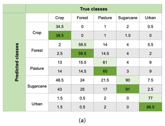
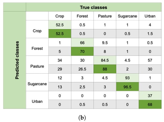
Figure 8.
Confusion matrix of (a) field-pixel and (b) field sampling; with SVM classifier: each cell included two values, where upper ones are only based on using intensity while the lower values are related to using intensity and coherence together.
4.2. Spatial Analysis
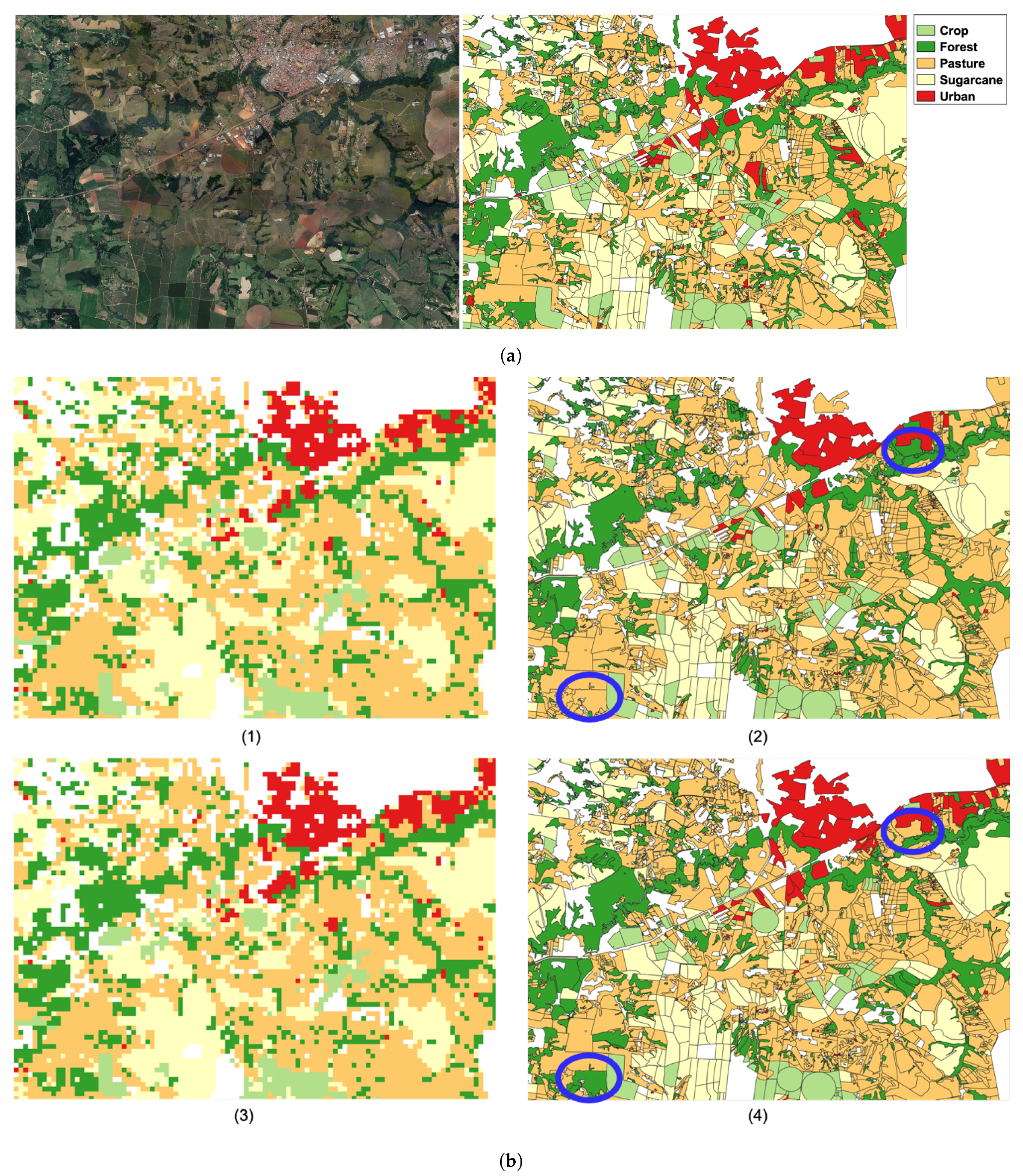
We analyze in more explicit spatial detail the output from the two most relevant feature configurations: (1) , —only backscattering coefficients are used; and (2) , , , —a combination of all SAR features is used. The classified maps are shown in Figure 9 for field pixel and field sampling schemes and the results related to the pixel sampling are not presented due to the fact that they include overfitting. As field sampling performs better according to the OA and confusion matrices, it is considered a reference for the remaining analysis in this paper. The blue circles in Figure 9b highlight two examples of fields presenting mixed pasture and forest pixels in the pixel-based classification maps, possibly denoting spatial heterogeneities not properly accounted for within the reference polygons. It can, however, be observed that the integration of the coherence in the field-based approach allows one to correctly identify the land cover majority, i.e., pasture cover for the upper field and forest for the lower one. From a qualitative standpoint, the classified maps convey that the two approaches are characterized by a substantial agreement which manifests in the difficulty to spot a total classification mismatch on large polygons. The differences between the pixel-based and the field-based polygons shall be rather found in single pixel errors (similarly to a salt and pepper noise). It is for instant evident in the presence of yellow (sugarcane) pixels in areas where no sugarcane is expected. This issue could be partly mitigated by the application of a majority filter as a post-processing step [38]. The use of such a filter on areas with small and medium parcels (compared to the sensor resolution), such as the one shown in Figure 9, however, could be detrimental and its impact should be more carefully investigated in future works.

Figure 9.
Comparison of the SVM classifier maps over a 10 × 7 km close-up of the study area: (a) reference data and (b) results from: (1) amplitude and field pixel sampling; (2) amplitude and field sampling; (3) amplitude + coherence and field pixel sampling; (4) amplitude + coherence and field sampling.
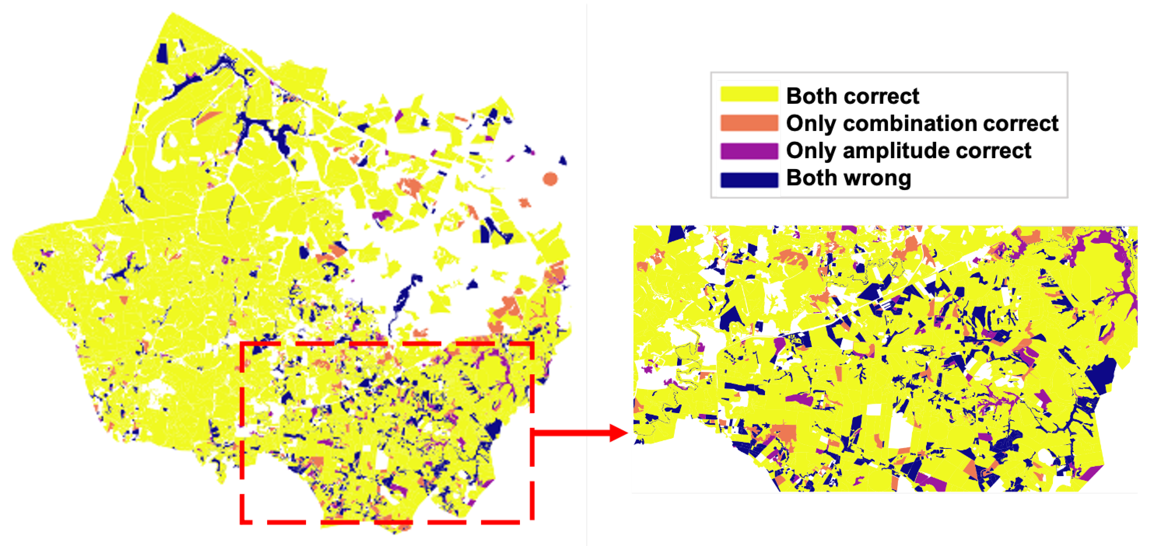
The impact of the coherence on the field-based classification is further highlighted by the differential map in Figure 10. The figure shows the whole area with four colors; the orange stands for those fields correctly classified only with the combined use of coherence and amplitude, where the purple represents correctly classified fields only by the exclusive use of the amplitude, and the yellow and the blue indicate the areas correctly and incorrectly classified in both configurations, respectively. The map conveys that the integration of the coherence does not only yield positive changes. Several fields are indeed correctly classified only when the single amplitude is used. In accordance with the performance in Table 2, it can be therefore inferred that the coherence introduces a small but significant noise in the classification output but that its effect is overall positive.
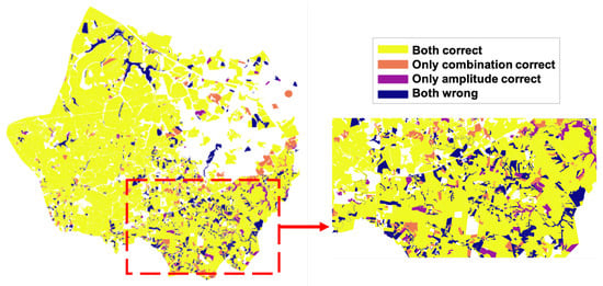
Figure 10.
Representation of match and mismatch, with respect to the ground truth, for the SVM-based maps obtained from intensity only and from the combination of intensities and coherence.
4.3. Feature Relevance Analysis
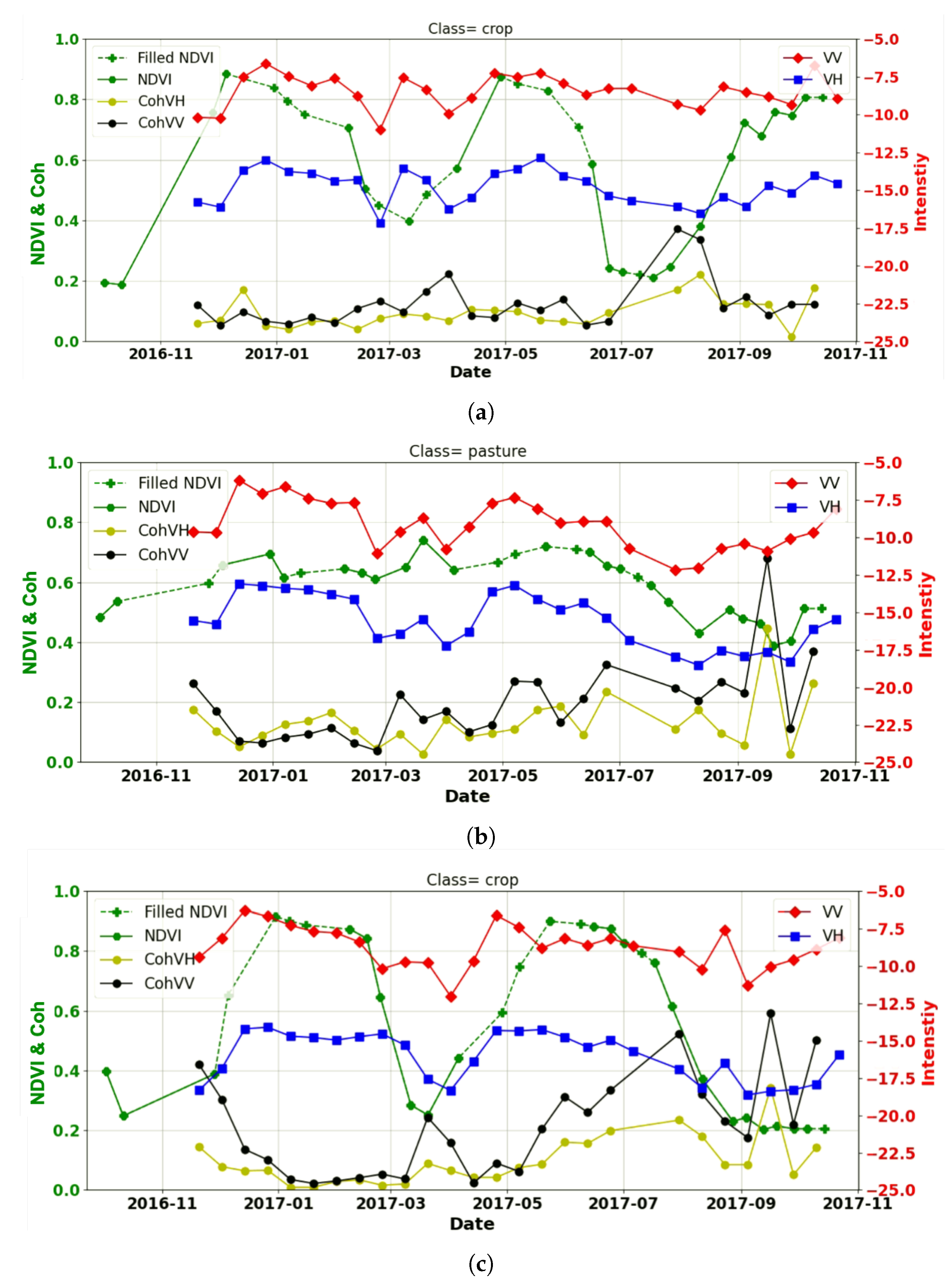
To illustrate the importance of the use of InSAR coherence information in land cover classification, the time-series of coherence and backscattered intensity in both channels was analyzed for those correctly classified fields only through the use of coherence in Figure 11a. The radar cross-polarized backscatter (VH) is known to be sensitive to the canopy volume, whereas it is less sensitive to the soil surface. The soil backscatter is stronger on the co-polarized signal (VV), which hence becomes a better proxy for soil moisture. However, both polarizations are sensitive to the water content of the medium, either in the soil or in the canopy, showing fluctuations after watering events (rain in our studied area) that can be used to infer information on the land cover conditions, as proven in [18]. Such fluctuations are clearly visible in Figure 11. From the panels, it is evident that the radar has a clear advantage over optical sensors in terms of temporal coverage, as the crop cycle is missed for some months by Landsat (the filled NDVI in the plot is the data that are estimated by interpolation). It can also be noticed that the radar signal is noisier, although, as already specified, part of the fluctuations has to be considered as water-related signal.
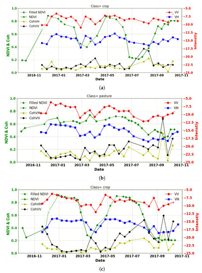
Figure 11.
SAR and optical time-series over different land covers: (a) for a field that is only correctly classified with the combined use of coherence and amplitude; (b) for a field that is only correctly classified by the exclusive use of the amplitude; and (c) for a field that is correctly classified with both configurations.
This first panel in Figure 11 shows that the coherence is sensitive to the harvest event in a crop field at the end of 2017, which appears as a sharp increase from a near zero value to approximately 0.4. Such clear change (a large backscatter drop is expected) cannot be found in the amplitude, which probably remains high either due to the straws in the field, or to possible enhanced Bragg scattering effects (although unlikely, since only VV would be expected to suffer from it) or to high moisture in the soil. It is likely that such sensitivity in the coherence is the key factor for enabling correct labeling from the algorithm.
Figure 11b corresponds to a pasture field that is classified correctly only with amplitudes. It is indeed confused by the algorithm with a crop field when the coherence is integrated. In light of the previous example, the confusion is introduced by the strong spike in coherence in September 2017, which is more characteristic for crop fields in bare soil state than for pasture fields. From the NDVI value closest to the spike, amounting to approximately 0.4, it can be inferred that the vegetation has sparse, dry or underdeveloped canopy, but it is not in bare soil state. The last panel in Figure 11c illustrates the time-series of a crop field which classified correctly both with and without the use of the coherence. In this case, both the coherence and the amplitude behavior clearly reveal the crop cycles, with two harvest events, the first in summer (at the end of March) and the second in winter (September). Notice a similar sensitivity in summer would also be expected from the first time-series (Figure 11a), as two distinct cycles can be identified from the NDVI. However, due to the fact that the harvest is performed on a portion of the field at a time, the bare soil condition is never reached on the whole reference polygon.
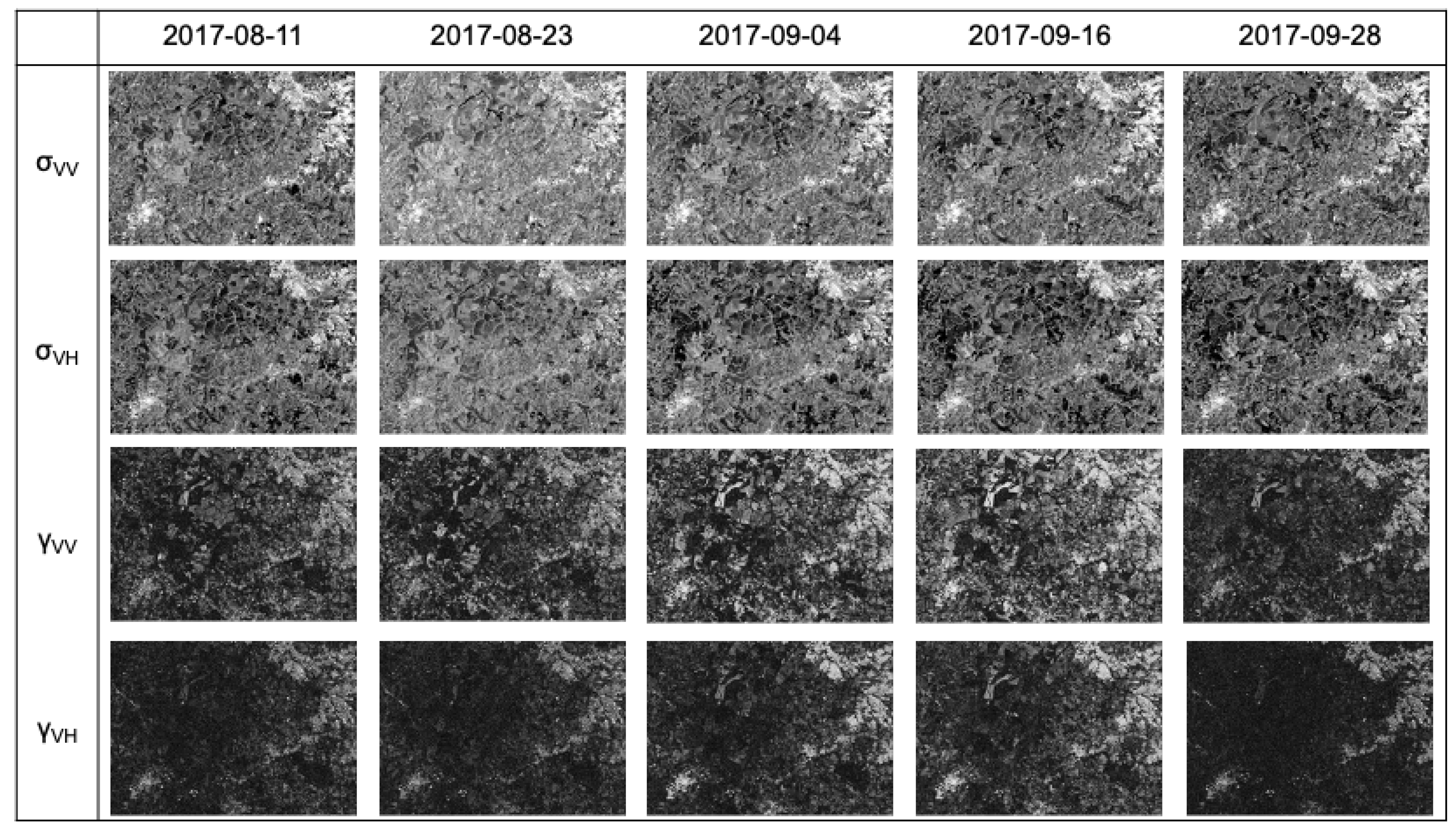
The coherences and the intensities in the two winter months of August and September are illustrated in Figure 12 with the aim of conveying, qualitatively, their partial complementary. At the beginning of August, the VH intensities and the coherences appear in a large part inversely correlated. However, it is possible to spot a few field locations with simultaneous moderate coherence and intensity values. This conveys that a minor, although significant, number of fields in senescence and post-harvest conditions can be exclusively identified through the coherence. The different sensitivity of the two features is further confirmed by the last acquisition of August (second column in the figure), where high backscatter values are registered over the whole image (possibly due to a rain event), including bare soil areas. It is interesting to notice that the coherence is instead only marginally affected, revealing, in this particular circumstance, an improved robustness.

Figure 12.
Images of coherence and intensities in the two winter months of August and September for both polarization. The coherence colors range from 0 (black) to 1 (white). The intensity values are shown in decibels. For the VV channel, the color range is set between −15 and −5 and for the VH channel it is set between −20 and −10. In all the images, lighter colors indicate higher values.
In order to have a deeper understanding of the added value of the feature integration, the feature selection is applied through mRMR based on the mutual information, as it was explained in Section 3.4. Table 3 reports the first four features selected by mRMR. For coherence, the date of the first SAR acquisition in the pair is reported. Notice that three out of the first four features are associated to winter acquisitions. The winter season is in fact the time of the year where the classes are most different.

Table 3.
First four selected features through the mutual information based mRMR.
Figure 13 illustrates the distributions of the high ranking features in Table 3 for the vegetation classes. The amplitude histograms in the first and in the fourth panel clearly convey that annual crops and sugarcane fields respond with lower backscatter, on average, than pasture fields. This offset is mainly due to the harvesting and ploughing operations that are often carried out on temporary and permanent crops. The two amplitude histograms similarly show that distinguishing between sugarcane and crop from a single amplitude image in winter is not possible, whereas the pasture and the forest have more distinct profiles.
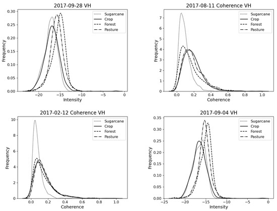
Figure 13.
Histograms of the vegetated classes for the four most relevant features, as can be seen in Table 3, as selected by the mRMR method.
The two coherence panels are associated with a dry period in summer (12–24 February) and a rain event in winter (11–23 August). The histogram of coherence in August is related to the period during which most of the annual crops and sugarcane are either harvested or in senescent conditions. As conveyed by Figure 3, the second acquisition in the pair (23 August) experiences an increase in amplitude that can be interpreted as the effect of rain during previous days. The historic rain data (both from weather stations and satellite) indeed confirm the occurrence of precipitations on the 19th and the 20th of August. The effect on VH is a generalized drop in the sugarcane coherence, whereas the impacts are not so evident for the other classes. For the sugarcane fields that are already harvested, this is due to the residues left on the ground, whereas for the fields in dry senescent state, the drop is caused by an increase in the canopy returns. Such a generalized response of sugarcane is less visible in the VV channel, where a significant portion of the harvested field manages to retain some coherence (see Figure 3). A similar behavior in the histograms can be observed for the February coherence, although with less separability between forest, pasture and crops. The reasons for the discrepancy between sugarcane and the other classes are, however, opposite in this feature, as the scene is illuminated at the end of a dry period in summer. The coherence values in summer are in fact extremely low for all classes and they incrementally rise during temporary droughts or after harvest events (for annual crop fields with double cropping management). Sugarcane fields are, however, less affected by such events since most of the fields are either in the vegetative or grand growth stages, characterized by high biomass and canopy water content [18]. The values therefore remain extremely low or null.
Two further aspects are worth noting. The first is that the analysis elaborated thus far led to general principles that hold for different areas and different years, as well as to quantitative outcomes that are strongly dataset dependent. For instance, the high relevance of the winter acquisitions is easily applicable to different case studies and dataset in Brazil. The double cropping consideration for the summer/spring acquisitions also fall in this category, when considered in a broad sense. However, the score and the exact date of these features shall be intended as area-, year- and dataset-specific and cannot be generalized. The second consideration concerns the low-class separability on single images, expressed by Figure 13. It is for instance not possible to distinguish between sugarcane and forest in winter, since not all the sugarcane fields are harvested at the same time. Such an issue conveys the need to use multi-temporal datasets and properly exploit the non-linear information of land cover events. Among these, the harvest event is deemed the key for the classification performance of both amplitudes and coherences.
5. Conclusions
In this paper, the added value of short-term coherence information in discriminating vegetation land covers was evaluated for Sentinel-1 dual-polarized SAR. The work was conducted on a site characterized by native vegetation and rain-fed pasture and crops, with a critical overlap of the class signatures in every amplitude and coherence feature.
Consistently with previous work, we found that the use of InSAR coherence leads to a significant improvement of the classification performances, for example, with improvements in the user accuracy for most classes considered in the order of 5 p.p. However, contrary to the results reported in [13], for our case study, we observed that the radar intensities guarantee higher separability than coherences by themselves.
The most sensitive information brought by coherence is found in the winter months, when crops are harvested, and during the short droughts in summer. In winter, the coherence increase experienced by annual crops help in discriminating them from forest and high grass pastures. During dry summer periods, the crops and the low grass pastures are then more likely to stand out from the near-null coherences of sugarcane.
The analysis further revealed that the capability of classifiers to exploit such a marginal amount of informative interferometric pairs (for sugarcane and pasture time-series, a single non-null coherence feature can be for instance observed) can significantly vary. In our case study, it was found that SVM classifiers are more effective than RF algorithms, although the improvements are only incremental. On such a note, it shall be specified that the impact of year-specific variables, i.e., the season-dependent weather and field management practices on the results is still poorly addressed, as only one season has been processed. The events leading to the complementary coherence information has been in fact effectively outlined, however, the extent of the associated performance improvement shall be object of further assessments.
A point of attention in the use of coherence time-series is that the coherences remain generally low throughout the time-series, making its estimation unreliable if the number of samples averaged to estimate it is low. The estimation of coherence on fields brings substantial performance improvement over conventional fixed-filter multi-looking.
A final recommendation from the study concerns the generation of training and validation data sets for pixel-based classification. Our position is that it is not sufficient to select a disjoint set of pixels for training and validation, but that the pixels used for training and validation should correspond to different fields. The analysis indeed conveys that failing to do so leads to substantial positive biases.
Author Contributions
T.N. conceived of and designed the study, designed the methodologies and implemented, validated, analyzed and interpreted the data and results and wrote the manuscript. L.I. and P.L.-D. assisted in designing the methodologies, analyzing the data, interpreting the results, reviewing and editing the manuscript. R.A.M. assisted in the interpretation of the results and in reviewing the manuscript. All authors have read and agreed to the published version of the manuscript.
Funding
This research received no external funding.
Institutional Review Board Statement
Not applicable.
Informed Consent Statement
Not applicable.
Acknowledgments
This project was undertaken in part within the framework of the FAPESP and NWO project. The authors would like to acknowledge the ESA for providing the Sentinel-1 data and NASA for providing the Landsat data. We would like to thank the colleague at TUDelft, Gert Mulder, for providing access to RIPPL. In addition, we would like to thank the colleagues at FEAGRI, Unicamp, for their assistance with taking the ground measurements together with the authors, in particular Diego della Justina, Carlos Wachholz de Souza, Walter Rossi Cervi, Rubens Lamparelli, Jansle Vieira Rocha and Ali Mousivand. Finally, we acknowledge and are grateful for the access to and safety in the sugarcane fields provided by Jefferson Rodrigo Batista de Mello, Eduaro Caetano Ceará, Pedro Lian Barbieri, and Alex Thiele Paulino.
Conflicts of Interest
The authors declare no conflict of interest.
References
- Strozzi, T.; Dammert, P.; Wegmuller, U.; Martinez, J.M.; Askne, J.; Beaudoin, A.; Hallikainen, N. Landuse Mapping with ERS SAR Interferometry. IEEE Trans. Geosci. Remote Sens. 2000, 38, 766–775. [Google Scholar] [CrossRef]
- Bruzzone, L.; Marconcini, M.; Wegmuller, U.; Wiesmann, A. An Advanced System for the Automatic Classification of Multitemporal SAR Images. IEEE Trans. Geosci. Remote Sens. 2004, 42, 1321–1334. [Google Scholar] [CrossRef]
- Torres, R.; Snoeij, P.; Geudtner, D.; Bibby, D.; Davidson, M.; Attema, E.; Potin, P.; Rommen, B.; Floury, N.; Brown, M.; et al. GMES Sentinel-1 Mission. Remote Sens. Environ. 2012, 120, 9–24. [Google Scholar] [CrossRef]
- Rodriguez-Galiano, V.F.; Ghimire, B.; Rogan, J.; Chica-Olmo, M.; Rigol-Sanchez, J.P. An Assessment of the Effectiveness of a Random Forest Classifier for Land-Cover Classification. ISPRS J. Photogramm. Remote Sens. 2012, 67, 93–104. [Google Scholar] [CrossRef]
- Shao, Y.; Lunetta, R.S. Comparison of Support Vector Machine, Neural Network, and CART Algorithms for the Land-Cover Classification Using Limited Training Data Points. ISPRS J. Photogramm. Remote Sens. 2012, 70, 78–87. [Google Scholar] [CrossRef]
- Diniz, J.M.F.d.S.; Gama, F.F.; Adami, M. Evaluation of Polarimetry and Interferometry of Sentinel-1A SAR Data for Land Use and Land Cover of the Brazilian Amazon Region. Geocarto Int. 2020, 1–19. [Google Scholar] [CrossRef]
- Gašparović, M.; Dobrinić, D. Comparative Assessment of Machine Learning Methods for Urban Vegetation Mapping Using Multitemporal Sentinel-1 Imagery. Remote Sens. 2020, 12, 1952. [Google Scholar] [CrossRef]
- Steele-Dunne, S.C.; McNairn, H.; Monsivais-Huertero, A.; Judge, J.; Liu, P.; Papathanassiou, K. Radar Remote Sensing of Agricultural Canopies: A Review. IEEE J. Sel. Top. Appl. Earth Obs. Remote Sens. 2017, 10, 2249–2273. [Google Scholar] [CrossRef] [Green Version]
- Ge, S.; Antropov, O.; Su, W.; Gu, H.; Praks, J. Deep Recurrent Neural Networks for Land-Cover Classification Using Sentinel-1 INSAR Time Series. In Proceedings of the IGARSS 2019—2019 IEEE International Geoscience and Remote Sensing Symposium, Yokohama, Japan, 28 July–2 August 2019; pp. 473–476. [Google Scholar] [CrossRef]
- Zalite, K.; Antropov, O.; Praks, J.; Voormansik, K.; Noorma, M. Monitoring of Agricultural Grasslands with Time Series of X-Band Repeat-Pass Interferometric SAR. IEEE J. Sel. Top. Appl. Earth Obs. Remote Sens. 2016, 9, 3687–3697. [Google Scholar] [CrossRef]
- Tamm, T.; Zalite, K.; Voormansik, K.; Talgre, L. Relating Sentinel-1 Interferometric Coherence to Mowing Events on Grasslands. Remote Sens. 2016, 8, 802. [Google Scholar] [CrossRef] [Green Version]
- Engdahl, M.; Hyyppa, J. Land-Cover Classification Using Multitemporal ERS-1/2 InSAR Data. IEEE Trans. Geosci. Remote Sens. 2003, 41, 1620–1628. [Google Scholar] [CrossRef]
- Jacob, A.W.; Vicente-Guijalba, F.; Lopez-Martinez, C.; Lopez-Sanchez, J.M.; Litzinger, M.; Kristen, H.; Mestre-Quereda, A.; Ziółkowski, D.; Lavalle, M.; Notarnicola, C.; et al. Sentinel-1 InSAR Coherence for Land Cover Mapping: A Comparison of Multiple Feature-Based Classifiers. IEEE J. Sel. Top. Appl. Earth Obs. Remote Sens. 2020, 13, 535–552. [Google Scholar] [CrossRef] [Green Version]
- Busquier, M.; Lopez-Sanchez, J.M.; Mestre-Quereda, A.; Navarro, E.; González-Dugo, M.P.; Mateos, L. Exploring TanDEM-X Interferometric Products for Crop-Type Mapping. Remote Sens. 2020, 12, 1774. [Google Scholar] [CrossRef]
- Sonobe, R.; Tani, H.; Wang, X.; Kobayashi, N.; Shimamura, H. Discrimination of Crop Types with TerraSAR-X-Derived Information. Phys. Chem. Earth Parts A/B/C 2015, 83–84, 2–13. [Google Scholar] [CrossRef] [Green Version]
- Sica, F.; Pulella, A.; Nannini, M.; Pinheiro, M.; Rizzoli, P. Repeat-Pass SAR Interferometry for Land Cover Classification: A Methodology Using Sentinel-1 Short-Time-Series. Remote Sens. Environ. 2019, 232, 111277. [Google Scholar] [CrossRef]
- Khalil, R.Z.; Saad-ul-Haque. InSAR Coherence-Based Land Cover Classification of Okara, Pakistan. Egypt. J. Remote Sens. Space Sci. 2018, 21, S23–S28. [Google Scholar] [CrossRef]
- Molijn, R.A.; Iannini, L.; López Dekker, P.; Magalhães, P.S.G.; Hanssen, R.F. Vegetation Characterization through the Use of Precipitation-Affected SAR Signals. Remote Sens. 2018, 10, 1647. [Google Scholar] [CrossRef] [Green Version]
- Molijn, R.A.; Iannini, L.; Rocha, J.V.; Hanssen, R.F. Author Correction: Ground Reference Data for Sugarcane Biomass Estimation in São Paulo State, Brazil. Sci. Data 2019, 6, 306. [Google Scholar] [CrossRef] [Green Version]
- Matsushita, B.; Yang, W.; Chen, J.; Onda, Y.; Qiu, G. Sensitivity of the Enhanced Vegetation Index (EVI) and Normalized Difference Vegetation Index (NDVI) to Topographic Effects: A Case Study in High-Density Cypress Forest. Sensors 2007, 7, 2636–2651. [Google Scholar] [CrossRef] [Green Version]
- Hao, D.; Wen, J.; Xiao, Q.; Wu, S.; Lin, X.; You, D.; Tang, Y. Modeling Anisotropic Reflectance Over Composite Sloping Terrain. IEEE Trans. Geosci. Remote Sens. 2018, 56, 3903–3923. [Google Scholar] [CrossRef]
- Farr, T.G.; Rosen, P.A.; Caro, E.; Crippen, R.; Duren, R.; Hensley, S.; Kobrick, M.; Paller, M.; Rodriguez, E.; Roth, L.; et al. The Shuttle Radar Topography Mission. Rev. Geophys. 2007, 45. [Google Scholar] [CrossRef] [Green Version]
- Seymour, M.; Cumming, I. Maximum Likelihood Estimation for SAR Interferometry. In Proceedings of the IGARSS’94—1994 IEEE International Geoscience and Remote Sensing Symposium, Pasadena, CA, USA, 8–12 August 1994; Volume 4, pp. 2272–2275. [Google Scholar] [CrossRef] [Green Version]
- Touzi, R.; Lopes, A.; Bruniquel, J.; Vachon, P. Coherence Estimation for SAR Imagery. IEEE Trans. Geosci. Remote Sens. 1999, 37, 135–149. [Google Scholar] [CrossRef] [Green Version]
- López-Martínez, C.; Pottier, E. Coherence Estimation in Synthetic Aperture Radar Data Based on Speckle Noise Modeling. Appl. Opt. 2007, 46, 544–558. [Google Scholar] [CrossRef]
- Touzi, R.; Lopes, A. Statistics of the Stokes Parameters and of the Complex Coherence Parameters in One-Look and Multilook Speckle Fields. IEEE Trans. Geosci. Remote Sens. 1996, 34, 519–531. [Google Scholar] [CrossRef]
- Hussain, M.; Chen, D.; Cheng, A.; Wei, H.; Stanley, D. Change Detection from Remotely Sensed Images: From Pixel-Based to Object-Based Approaches. ISPRS J. Photogramm. Remote Sens. 2013, 80, 91–106. [Google Scholar] [CrossRef]
- Addink, E.A.; Van Coillie, F.M.B.; De Jong, S.M. Introduction to the GEOBIA 2010 Special Issue: From Pixels to Geographic Objects in Remote Sensing Image Analysis. Int. J. Appl. Earth Obs. Geoinf. 2012, 15, 1–6. [Google Scholar] [CrossRef]
- Cortes, C.; Vapnik, V. Support-Vector Networks. Mach. Learn. 1995, 20, 273–297. [Google Scholar] [CrossRef]
- Breiman, L. Random Forests. Mach. Learn. 2001, 45, 5–32. [Google Scholar] [CrossRef] [Green Version]
- Pedregosa, F.; Varoquaux, G.; Gramfort, A.; Michel, V.; Thirion, B.; Grisel, O.; Blondel, M.; Prettenhofer, P.; Weiss, R.; Dubourg, V.; et al. Scikit-Learn: Machine Learning in Python. J. Mach. Learn. Res. 2011, 12, 2825–2830. [Google Scholar]
- Kavzoglu, T.; Colkesen, I. A Kernel Functions Analysis for Support Vector Machines for Land Cover Classification. Int. J. Appl. Earth Obs. Geoinf. 2009, 11, 352–359. [Google Scholar] [CrossRef]
- Stehman, S.V. Selecting and Interpreting Measures of Thematic Classification Accuracy. Remote Sens. Environ. 1997, 62, 77–89. [Google Scholar] [CrossRef]
- Peng, H.; Long, F.; Ding, C. Feature Selection Based on Mutual Information Criteria of Max-Dependency, Max-Relevance, and Min-Redundancy. IEEE Trans. Pattern Anal. Mach. Intell. 2005, 27, 1226–1238. [Google Scholar] [CrossRef] [PubMed]
- Ding, C.; Peng, H. Minimum Redundancy Feature Selection from Microarray Gene Expression Data. In Proceedings of the 2003 IEEE Bioinformatics Conference, Computational Systems Bioinformatics (CSB2003), Stanford, CA, USA, 11–14 August 2003; pp. 523–528. [Google Scholar] [CrossRef]
- Ding, C.; Peng, H. Minimum Redundancy Feature Selection from Microarray Gene Expression Data. J. Bioinform. Comput. Biol. 2005, 3, 185–205. [Google Scholar] [CrossRef] [PubMed]
- Mestre-Quereda, A.; Lopez-Sanchez, J.M.; Vicente-Guijalba, F.; Jacob, A.W.; Engdahl, M.E. Time Series of Sentinel-1 Interferometric Coherence and Backscatter for Crop-Type Mapping. IEEE J. Sel. Top. Appl. Earth Obs. Remote Sens. 2020, 13, 4070–4084. [Google Scholar] [CrossRef]
- Cué La Rosa, L.E.; Queiroz Feitosa, R.; Nigri Happ, P.; Del’Arco Sanches, I.; Ostwald Pedro da Costa, G.A. Combining Deep Learning and Prior Knowledge for Crop Mapping in Tropical Regions from Multitemporal SAR Image Sequences. Remote Sens. 2019, 11, 2029. [Google Scholar] [CrossRef] [Green Version]
Publisher’s Note: MDPI stays neutral with regard to jurisdictional claims in published maps and institutional affiliations. |
© 2021 by the authors. Licensee MDPI, Basel, Switzerland. This article is an open access article distributed under the terms and conditions of the Creative Commons Attribution (CC BY) license (https://creativecommons.org/licenses/by/4.0/).

