Abstract
Vegetation phenology is an integrative indicator of environmental change, and remotely–sensed data provide a powerful way to monitor land surface vegetation responses to climatic fluctuations across various spatiotemporal scales. In this study, we synthesize the local climate, mainly temperature and precipitation, and large-scale atmospheric anomalies, El Niño-Southern Oscillation (ENSO)-connected dynamics, on a vegetative surface in a subtropical mountainous island, the northwest Pacific of Taiwan. We used two decadal photosynthetically active vegetation cover (PV) data (2001–2020) from Moderate Resolution Imaging Spectroradiometer (MODIS) reflectance data to portray vegetation dynamics at monthly, seasonal, and annual scales. Results show that PV is positively related to both temperature and precipitation at a monthly timescale across various land cover types, and the log-linear with one-month lagged of precipitation reveals the accumulation of seasonal rainfall having a significant effect on vegetation growth. Using TIMESAT, three annual phenological metrics, SOS (start of growing season), EOS (end of growing season), and LOS (length of growing season), have been derived from PV time series and been related to seasonal rainfall. The delayed SOS was manifestly influenced by a spring drought, <40 mm during February–March. The later SOS led to a ramification on following late EOS, shorter LOS, and reduction of annual NPP. Nevertheless, the summer rainfall (August–October) and EOS had no significant effects on vegetation growth owing to abundant rainfall. Therefore, the SOS associated with spring rainfall, instead of EOS, played an advantageous role in regulating vegetation development in this subtropical island. The PCA (principal component analysis) was applied for PV time series and explored the spatiotemporal patterns connected to local climate and climatic fluctuations for entire Taiwan, North Taiwan, and South Taiwan. The first two components, PC1 and PC2, explained most of data variance (94–95%) linked to temporal dynamics of land cover (r > 0.90) which was also regulated by local climate. While the subtle signals of PC3 and PC4 explained 0.1–0.4% of the data variance, related to regional drought (r = 0.35–0.40) especially in central and southwest Taiwan and ENSO-associated rainfall variation (r = −0.40–−0.37). Through synthesizing the relationships between vegetation dynamics and climate based on multiple timescales, there will be a comprehensive picture of vegetation growth and its cascading effects on ecosystem productivity.
1. Introduction
The dynamics of vegetation growth or phenology, (i.e., the timing and duration of vegetation activity across a year) which plays a crucial role in regulating the water cycle, carbon cycle, energy balance, biomass accumulation, and productivity largely depends on key climatic factors, temperature, precipitation, and radiation [1,2,3]. Identifying vegetation phenology and their responses to climatic and non-climatic factors has recently become a central issue in the studies of global change biology/ecology and biogeochemistry. Many studies have shown that temperature is the dominant control of plant growth in high latitudes and cold regions, precipitation is the dominant factor in arid and semiarid areas, whereas radiation is key to plant growth in rainforest [4,5,6,7]. However, compared to abundant reports from various parts of mid- and high-latitudes, our knowledge about vegetation-climate dynamics in tropics/subtropics is mainly from the Amazon basin in South American and the Congo rainforest in Africa [8,9,10,11]. More efforts are required to provide a better understanding of vegetation-climate dynamics for isolated islands in tropical and subtropical regions, where there are hotspots of biological diversity that are more susceptible due to their unique environment and limited area [12].
In situ field observations can provide detailed information of plant growth at the species level and efforts have been made to provide large scale field observation across many countries, such as the National Phenology Network of USA (https://www.usanpn.org/, accessed on 7 July 2021) [13], the International Phenological Gardens of Europe (http://ipg.hu-berlin.de/, accessed on 7 July 2021) [14], and the Chinese Phenological Observation Network (http://www.cpon.ac.cn/, accessed on 7 July 2021) [15]. However, field works are time-consuming and labor-intensive, such that they are only monitored on a small spatial scale in each site. In contrast, satellite-derived vegetation indices (VIs), such as normalized difference vegetation index (NDVI) and enhanced vegetation index (EVI), have been widely utilized to characterize vegetation growth in relation to climatic parameters. The VIs can also be used to calculate key phenological metrics known as land surface phenology (LSP), including the start of growing season (SOS), end of growing season (EOS), and length of growing season (LOS) at regional and global scales [16,17,18]. The successful detections of phenological patterns and their variation from landscape to global levels have demonstrated that the satellite data can serve as a useful and reliable means to disentangle how vegetation phenology responds to climate change on a broader scale [19,20]. The advanced very high-resolution radiometer (AVHRR; 1.1 km in spatial resolution) and the successive monitoring sensor Moderate Resolution Imaging Spectroradiometer (MODIS; 250 m–1000 m in spatial resolution) have provided datasets for more than three decades with a high capability for regional vegetation-climate monitoring and ecosystem process modeling [21,22,23,24]. Chang et al. [25] indicated that MODIS NDVI and EVI positively related to both temperature and precipitation on a monthly timescale, but were not significant at the annual timescale in subtropical Taiwan, and suggested that the finer spatial and temporal scales could be better to reveal the climatic controls over vegetation growth. Besides, the time-lag effect of vegetation responses to temperature and precipitation was commonly observed for various land covers. A time lag of one to three months should be considered when exploring the associations of vegetation growth with local climate [7,26,27,28].
The seasonal phenological metrics, i.e., SOS, EOS, and LOS, calculated from time-series satellite images have been continuously and extensively utilized to detect the vegetation responses of specific phases to climatic change or disturbances over the last two decades [29,30,31]. For example, the SOS and/or EOS of forests in Europe and eastern USA is dominated by temperature [31,32]. The spatiotemporal patterns of SOS and EOS in the Tibetan Plateau are determined by the combined effects of temperature, altitude, snow cover, and photoperiod [15]. Previous evaluations show that longer extension of LOS significantly relates to advanced SOS [33,34,35]. However, several studies have exhibited the contrast results that the SOS shows a slower advanced rate or delayed after 2000 due to drought and deficiency of soil moisture [36,37], and climate extremes [38]. Further analysis is necessary to ascertain this trend at a regional scale because the interannual variability of LSP is changing with the warming climate. It is fundamental to track the dynamics of vegetation growth over time with longer records of remotely sensed and climate data.
Compared to most research conducted on the relationships between vegetation growth and local climatic factors [25,39,40], few studies have examined the dynamics of regional vegetation growth to large-scale climatic variations, such as the El Niño-Southern Oscillation (ENSO) which might influence vegetation dynamics through its combined effects on temperature, rainfall, drought, cloud cover, and subsequent solar radiation [41]. The ENSO warm (El Niño) years are usually related to decreased precipitation and freshwater discharges over many continents; in contrast, the ENSO cold (La Niña) years can contribute to wetter conditions [42]. Global studies indicated that El Niño years could lead to a reduction of greenness, productivity, and mortality in northeastern South America, Southeast Asia, Australia, and southern Africa, but increased land surface greenness in northern America, central Asia, and eastern Africa, and vice versa for La Niña years [43,44]. To decipher the effects of climatic fluctuation on vegetation dynamics, the multivariate statistical approach principal component analysis (PCA) is commonly applied to analyze space-time variance of vegetative land surface and characterize its major and hidden patterns from a given large image dataset [45,46,47,48]. Several studies conducted on continental and global scales have manifested that the first principal component (PC1) accounts for the largest variance of the major element in the time series of VI associated with steady land cover types, while the subsequent PC images with lower variations could delineate interannual variability of VI related to anthropogenic intervention and climate anomalies including rainfall interannual variability and ENSO cycles [49,50,51]. However, very few studies provide a comprehensive understanding of vegetation dynamics responses to key climate and non-climate factors at multiple time scales, i.e., monthly, seasonal, and annual.
Taiwan, a humid subtropical mountainous island with high annual precipitation (MAP) approximate 2500 mm year−1, has experienced an amplifying seasonal rainfall and droughts (i.e., drier winter-spring and wetter summer), and regional discrepancies between wetter northern Taiwan and drier southern Taiwan over the past century [52,53]. Studies have demonstrated that the El Niño events during the preceding winter (November–February) will bring abundant rainfall for the following spring and summer seasons in Taiwan, and vice versa for La Niña events [54,55]. The changing local climate and climate varieties will cause significant impacts on vegetation activity, carbon sequestration, and productivity in the region sensitive to climate dynamics [56,57]. Therefore, in this study, we will utilize MODIS, local climate, and large-scale climate anomaly datasets for two decades (2001–2020) to synthesize the vegetation response to short-term (monthly), seasonal, and interannual climatic variations in Taiwan. The objectives of this study are to (1) understand the relationships between vegetation activity and temperature and precipitation across various land cover types on a monthly time scale, (2) explore the effects of seasonal rainfall, spring rainfall and summer rainfall, on phenological patterns (SOS, EOS, and LOS) and their impacts on productivity, and (3) examine interannual variations of vegetation activity in relation to anthropogenic and climatic factors.
2. Materials and Methods
2.1. Study Area
Taiwan, a subtropical mountainous island with 36,000 km2 in area, is located between the largest continent (Eurasia) and the largest ocean (Pacific) (Figure 1a). Elevation increases from sea level to approximately 4000 m in a horizontal distance <75 km. The Tropic of Cancer runs across central Taiwan and divides it into subtropical and tropical monsoon climatic zones. High temperature (21 °C of annual mean temperature [MAT]), precipitation (2450 mm of mean annual precipitation [MAP]) and humidity, and frequent typhoons in summer-autumn characterizes the general climate pattern of Taiwan. The MAT decreases with elevation, while MAP generally increases with elevation and up to 4500 mm year−1 at high altitude and northeastern Taiwan and decreases to less than 1500 mm year−1 in the southwestern coastal plain (Figure 1b) [25]. There are more than 75% of MAP falling during summer (May–October), whereas winter-spring is relatively dry especially in southwestern Taiwan as it is on the leeside of the Central Mountain Range during prevailing northeast monsoons (Figure 1b).
The island-wide principal land use and vegetation types gradually change along an elevation gradient from urban-buildup and farmland on plains (<800 m a.s.l.), an evergreen broadleaved forest at low- and mid-elevation (200–2000 m a.s.l.), and mixed and conifer forests at mid- and high-elevation (>1100 m). Forests and agricultural land cover approximately 60% and 27% of the land area in Taiwan, the remaining 13% includes urban, villages, roads, streams, waterbody, beaches, and so on (Figure 1c) [25,58]. The logging of natural forests has been abandoned in Taiwan since 1991, and there is no anthropogenic interference, so the background of the diverse bioclimatic gradient is an ideal place for evaluating vegetation dynamics connecting to local climate and large-scale climatic fluctuations in the subtropical region.

Figure 1.
The geographical local map of the study region (Taiwan). (a) the distribution of climate stations, mean annual precipitation (MAP, contours), the average of vegetation cover fraction calculated from MODIS surface reflectance data (MOD09A1) in background [59], and the monthly climate chart which is the average value calculated from all climate stations during 2001–2020 (b), and land cover types in Taiwan (c).
2.2. Data Aquirement and Processing
2.2.1. Photosynthetic Active Vegetation (PV)
Two tiles (H28V06 and H29V06) of MODIS 8-day 500 m spatial resolution surface reflectance product (MOD09A1) on the Terra platform for the study period during 2001–2020 were retrieved from the NASA Land Processes Distributed Active Archive Center (LP DAAC; https://lpdaac.usgs.gov/tools/data-pool/, accessed on 5 June 2021). The spectral mixture analysis (SMA) has been commonly conducted [58,60] to decompose image pixels into three main surface components, i.e., PV (photosynthetic active vegetation), NPV (non-photosynthetic active vegetation), and SRO (soil and rock outcrop). This automated probability-based method was used to obtain the proportions of sub-pixel cover fractions of each endmember (PV, NPV, and SRO) [60]. A set of spectral libraries which was needed for the spectral unmixing (nPV = 580, nNPV = 267, and nSRO = 256). Endmembers for NPV and SRO were directly sampled using a field spectroradiometer (FiedSpec 3, ASD Inc., Boulder, CO, USA). Due to the high density of the vegetation canopy in Taiwan, PV endmember was collected from 25 spaceborne hyperspectral Hyperion images using manual delineation to select vegetation spectra. Then, the measurements were convoluted to match the MODIS spectral profiles [59]. A total of 240 monthly PV images were derived from 920 images (3–4 images per month) between 2001 and 2020 based on the maximum value composite (MVC) method [61]. We utilized PV instead of commonly used NDVI or EVI because PV is very sensitive to vegetation cover and to monthly mean air temperature and monthly precipitation than NDVI or EVI [62]. Besides, the PV was calculated based on spectral mixture analysis to extract the sub-pixel information to reduce spectral mixture problems [60].
Annual MODIS NPP (MOD17A3HGFv006) 500 m products for 20 years were also acquired from LP DAAC and were compared to the following seasonal rainfall and three phenological metrics. The MODIS NPP products have been successfully applied in assessing regional food supply, agricultural growing season, and ecosystem plant production [63,64].
2.2.2. Land Cover Data
The land cover classification data was acquired from the National Land Surveying and Mapping Center in Taiwan (Figure 1c; https://maps.nlsc.gov.tw/, accessed on 13 January 2021), which was essential for PV-climate analysis and was provided as input for phenological analysis. The digital map was created based on aerial photographs and satellite data, then continuously validated with field survey after 2008 [65]. We selected sampling sites including at least 0.1% of the area of each land use/vegetation type, in which the criteria of a selected site should be 2–5 times of the area of an image pixel to avoid problems by registration error as suggested by Muchoney et al. [66]. There were 830 points selected in total to extract monthly PV, temperature, and precipitation. For phenological metrics analysis, land cover types were supplied as background parameters setting in curve fitting for image time series in TIMESAT.
2.2.3. Climate Data and ENSO
Monthly temperature (n = 136) and precipitation (n = 390; Figure 1b) data during 2001–2020 were acquired from the Data Bank of Atmospheric and Hydrologic Research of Taiwan (https://dbar.pccu.edu.tw/, accessed on 12 May 2021). The monthly temperature layers were estimated by elevation, latitude, and longitude using a multiple linear regression as mentioned [67]. The monthly precipitation (MP) layers were generated applying the ordinary Kriging interpolation with a spherical model in ArcGIS v.10.6 (ESRI, Inc., Redlands, CA, USA) [58]. The output resolution of monthly temperature and precipitation data was 500 m × 500 m, consistent with the MODIS images. In order to find out the best relationships between seasonal rainfall and phenological metrics, various combinations of monthly precipitation (December, January, February, March, and April), summation of two-month precipitation (December–January, January–February, February–March, and March–April), and summation of three-month precipitation (December–February, January–March, and February–April) during winter-spring periods were used to related to SOS, EOS, LOS, and NPP. The monthly precipitation (July, August, September, October, and November), two-month precipitation (July–August, August–September, September–October, and October–November), and three-month precipitation (July–September, August–October, September–November) during summer-autumn periods were used to related to EOS, LOS, and NPP. See Section 2.5. Statistical Analysis for determination of the final model.
To portray the precipitation variability during 2001–2020 in Taiwan, we calculated the standardized precipitation index (SPI) based on MP with a three-month time scale (SPI3) to detect the drought conditions in the region as proposed by Chen et al. [52]. Based on the long-term data over the last century, Chen et al. [52] found that SPI3 could best characterize different drought severities, durations, and separated regional divergences of incidence of meteorological drought, i.e., decreased in northern Taiwan and increased in southern Taiwan. The SPI was defined as the transformation of MP time series into a standardized normal distribution (z-distribution):
where , , and are the precipitation for month i, mean and standard deviation of MP, respectively, over the study period [68,69]. Positive and negative values of SPI stand for wet and dry conditions, respectively, which is suitable for identifying most types of drought events at various regions [68,69].
The Southern Oscillation Index (SOI) is widely used to evaluate ENSO which considers the measurements of atmospheric pressure at sea level between Darwin in Northern Australia and Papeete in Tahiti. The negative (<−1.0) and positive (>1.0) SOI signals indicate warm (El Niño) and cold (La Niña) events, respectively [70]. Previous studies showed that the dynamics of SOI are associated with seasonal precipitation amount and anomalies across tropics and subtropics [71,72,73]. The monthly SOI for the study period 2001–2020 was obtained from ESNO information of NOAA Physical Sciences Laboratory (https://psl.noaa.gov/enso/, accessed on 19 June 2021) to examine its relationship with potential PCA loadings derived from PV image time series.
2.3. Phenological Metrics Calculation
Three primary phenological metrics, SOS, EOS, and LOS, were obtained from a 20-year MODIS PV time series using TIMESAT v3.3 (https://web.nateko.lu.se/timesat/timesat.asp?cat=0, accessed on 7 April 2020) developed by Jönsson and Eklundh [74] because it is commonly used for computing land surface phenology [75,76]. A smoothing approach is necessary to retain temporal details by excluding unusual high or low vegetation indexes. There are many smoothing methods available such as best index slope extraction (BISE) [77], Fourier transform [78], logistic function [79], piecewise logistic functions [80], Savitzky–Golay filter [81], etc. TIMESAT tool package provides several mathematical fitting functions for working out temporal dynamics of vegetation growth (Figure 2).
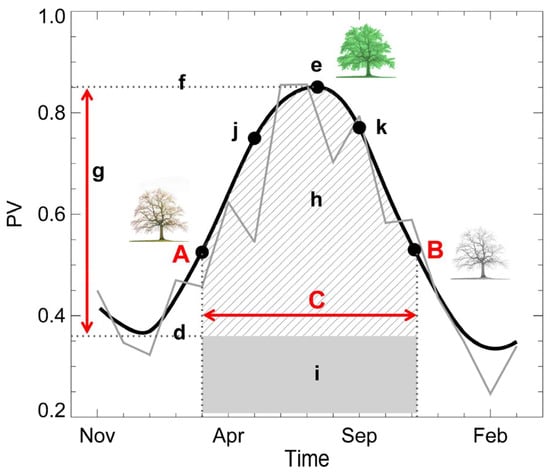
Figure 2.
The phenological metrics obtained from a smoothed curve (dark think line) of a time series of photosynthetically active vegetation (PV, gray line) using the TIMESAT tool. Three major metrics are derived from the time series of images: A—SOS (start of growing season), B—EOS (end of growing season), and C—LOS (length of growing season). d—base value, e—time of middle season, f—maximum value, g—amplitude, h—small integrated value, h+i—large integrated value (showing the cumulative effect of vegetation growth during the season), and j and k are 80% of level of left and right side curve respectively.
The Savitzky–Golay (SG) filter was determined because it can best preserve the temporal vegetation dynamics and minimize the atmospheric contamination and has been successfully applied in studies of different regions [58,81,82,83], which has also been integrated into the processing of the MODIS phenology product [84]. The SG filter can be expressed as below:
where is the original PV, is the outcome PV value, is the coefficient for the ith PV of the smoothing window, N is the number of convoluting integers which is equal to the smoothing window size (2m + 1), j stands for the running index of the ordinate data in the original data table, and m exhibits the half-width of the smooth window [81,82]. Using PV time series and supplementary land-cover settings (see [85] for detail), we can calculate the land surface phenological metrics, SOS (A, presented as the Julian date [JD]), EOS (B, presented as the Julian date [JD]), and LOS (C, presented as the days) (Figure 2), for each year. The relationships among the annual SOS, EOS, LOS, spring rainfall, summer rainfall, and annual MODIS NPP were examined.
2.4. Principal Component Analysis of Time-Series Images
In order to investigate the leading fundamental modes of variances from the 20-year PV time series of images, principal component analysis (PCA) was implemented to eliminate redundant information so that only the most dominant spatiotemporal patterns are retained in which cumulative variance can account for >95% of the variability of the original dataset [86,87]. This multivariate statistical technique transforms a group of correlated PV images into a set of uncorrelated variables, called principal components (PCs) consisting of spatial patterns of eigenvectors derived from original time-series images, and temporal loadings the coefficients of linear combinations that presents the correlations of original variables in PCs [88]. The eigenvectors indicated the weight of each one of the 240 images which were used to obtain factor loadings [49]. The correlation matrix was adopted (standardized PCA) to give the same weight for each image in the processing and to detect better and new spatial and temporal patterns [89]. Eigenvalues, used to detect the percentage of variation for each PC, were generated when the PCA process is completed with ENVI 5.5 (Research Systems, Boulder, CO, USA). The temporal loadings of each PC can be calculated as follow:
where is a loading value of each component i with each input date k, is eigenvector for component i with each input data k, and is eigenvalue for each component [90].
To properly explain the spatiotemporal patterns of PCA, we compared each PC image and its temporal loadings included the time-lag effect to look for feasible spatiotemporal associations such as the phenology of land cover, SPI3, SOI, or minor unrecognizable noise. Only significant relationships (|r| > 0.3, p < 0.05) between component loadings and variables are kept finally. Due to the increasing incidence of meteorological drought in southern Taiwan and decreasing incidence of drought in northern Taiwan [52], the PV images of subtropical North Taiwan (N Taiwan) and tropical South Taiwan (S Taiwan), separated by the Tropic of Cancer, were also conducted by PCA to find out the regional differences of vegetative surface responses to related variables.
2.5. Statistical Analysis
The simple linear regression and non-linear regression models, such as logarithm, exponential growth, and power-law equation, are used to explore the relationships between monthly PV and monthly temperature and precipitation, in which the moving averages of preceding one- and two-months and concurrent monthly climate are utilized to detect the lag effect between temperature/precipitation and PV [26,27], i.e., concurrent monthly (lag0), moving average of concurrent and preceding one monthly (lag1), and moving average of concurrent and preceding two months (lag2) temperature or precipitation. The multiple stepwise regression analysis was further applied to examine which variables could best explain the variability of PV. The variance of inflation factor (VIF) < 10 was used to avoid multi-collinearity among variables in the final models. The finally best fit linear, non-linear, and stepwise regression model was determined by the highest determination coefficient (R2) with a statistical significance at p-value < 0.05. Regression models are also applied to investigate the relationships among spring rainfall, summer rainfall, three annual phenological metrics (SOS, EOS, LOS), and NPP, and the relationships between temperature/precipitation and potential PCA loadings.
3. Results
3.1. Monthly PV-Climate Relationships
The average PV of 20 years across Taiwan increased from <0.10 at the west coastal region to >0.80 at the mid- and high-elevation forested regions (Figure 1b). The temporal PV showed similar patterns across all land cover types, rising in spring, reaching a maximum during June–August, then gradually decreasing to a minimum during January–March (Figure 3a). The PV of different land cover types varied considerably, lowest in urban (0.16–0.40), followed by paddy field (0.23–0.80), grassland (0.38–0.86), rainfed farmland (0.45–0.88), conifer forests (0.52–0.83), mixed forests (0.53–0.95), and highest in the broadleaved forest (0.58–0.98) (Figure 3a).
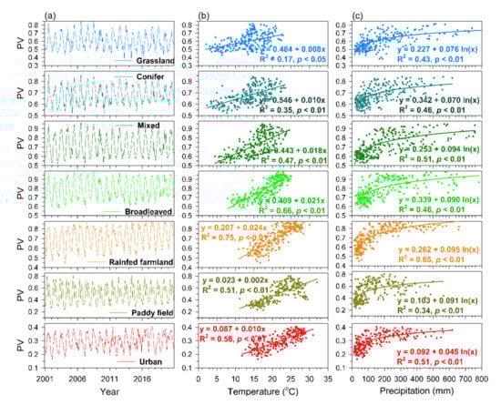
Figure 3.
The temporal dynamics of monthly PV during 2001–2020 (a), the relationships between monthly mean temperature and monthly PV (no time lag; lag0) (b), and the relationships between monthly precipitation and monthly PV (lagged one month; lag1) (c) for individual vegetation/land use types (n = 240 months).
The monthly PV had a significant positive relationship with concurrent monthly temperature without time-lag for individual vegetation/land cover types (Figure 3b). The coefficient of determination (R2) of linear regressions was 0.17 for grassland, 0.35 for conifer forests, 0.47 for mixed forests, 0.66 for broadleaved forests, 0.75 for rainfed farmland, 0.51 for paddy field, and 0.58 for urban (Figure 3b). By contrast, the monthly PV had a significant log-linear relationship with one-month lagged of precipitation (lag1) for all vegetation/land cover types, in which the higher PV was associated with greater rainfall within the range of 0–100 mm of precipitation, above 100 mm of precipitation the relationship leveled off (Figure 3c). The R2 of the log-linear regressions was 0.43 for grassland, 0.46 for conifer forests, 0.51 for mixed forests, 0.46 for broadleaved forests, 0.65 for rainfed farmland, 0.34 for paddy field, and 0.51 for urban (Figure 3c). The stepwise regression models with the highest R2 for estimating monthly PV ranged from 0.46 (grassland) to 0.71 (broadleaved forest) in which both concurrent temperature and precipitation with a one-month time lag (Plag1) were significant variables, except for paddy field having concurrent temperature the only significant variable (Table 1). The concurrent monthly temperature could explain most variability of monthly PV (40–68%), while the precipitation with a one-month time lag (Plag1) played a minor role in explaining variability (2–19%) of monthly PV (Table 1).

Table 1.
The stepwise regression models established by monthly PV, concurrent monthly temperature (T), and moving average of concurrent and preceding one-monthly precipitation (Plag1).
3.2. Influences of Seasonal Rainfall on Land Surface Phenology
The spatial patterns of SOS in Taiwan varied from <JD 80 to 160, with earlier SOS usually in the west plain and later SOS in the mid- to high-altitude areas (1500–2000 m) (Figure 4). The EOS varied from as early as JD 250 (early August) in the western plain where majorly occupied by farmland to as late as JD 350 (mid-December) at forested regions in mid-altitudes of southwestern and southeastern Taiwan (Figure 4). The LOS, determined by the difference between EOS and SOS, increased from <150 days in the west plain, 160–180 days at high-altitudes to >200 days at low- and mid-altitudes in southwestern Taiwan (Figure 4).
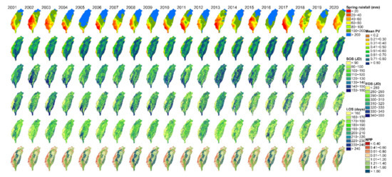
Figure 4.
From top to bottom: the spatial distribution of spring rainfall (February–March, mm), annual mean photosynthetically active vegetation (PV), SOS (start of growing season, Julian date, JD), EOS (end of growing season, Julian date, JD), LOS (length of growing season, days), and annual net primary productivity (NPP; kg C m−2 year−1) between 2001 and 2020.
The long-term mean (± SD) of annual MODIS NPP was 1.30 (±0.31) Kg C m−2 year−1, ranging from 1.27 (±0.32) Kg C m−2 year−1 in 2020 to 1.40 (±0.31) Kg C m−2 year−1 in 2009 (Figure 4). Along the elevational gradient, the NPP ascended from <0.6 Kg C m−2 year−1 in the coastal plain to >1.6 Kg C m−2 year−1 at 500–1500 m a.s.l., and then descended to approximate 1.0 kg C m−2 year−1 at >2500 m a.s.l., (Figure 4). The spatial patterns of SOS, EOS, and LOS showed clear inter-annual variations, but there was not a significant trend of mean SOS, EOS, LOS, and NPP of the entire study region over the two decades.
For the average values of forested region of island-wide scale, the increased spring rainfall was associated with an advanced SOS (r = −0.55, p < 0.05), a longer LOS (r = 0.63, p < 0.01), and a higher NPP (r = 0.74, p < 0.01; Figure 4 and Figure 5a–c). However, there was not a significant correlation found between spring rainfall and EOS. The earlier SOS significantly related to an earlier EOS (r = 0.74, p < 0.01), a longer LOS (r = –0.56, p < 0.05), and a higher NPP (r = –0.74, p < 0.01; Figure 5d–f). A longer LOS significantly related to a higher NPP (r = 0.62, p < 0.01; Figure 5g), but a later annual EOS would decrease annual NPP (r = –0.45, p < 0.05; Figure 6e). The rainfall quantity during summer had no significant correlations to mean EOS, LOS, and NPP (Figure 6a–c), neither correlation between EOS and LOS (Figure 6d). The spatial patterns of SOS and EOS and their relationships to spring rainfall and summer rainfall were further inspected during 2001–2020 (Figure 4). The regions of later SOS (late May, >JD 150) were consistent with the regions (42–85% of agreement) that received spring rainfall <40 mm, mostly in the west and southwest Taiwan where were susceptible to drought conditions. Nevertheless, there was not a clear picture between interannual variations of EOS and summer rainfall owing to the plentiful amount of precipitation during summer growing seasons (>500 mm; Figure 6).
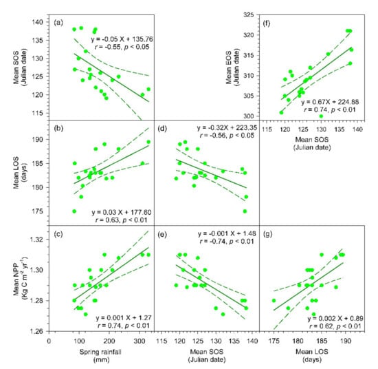
Figure 5.
The relationships between spring rainfall (February–March) and the mean SOS (a), mean LOS (b), and the mean NPP (c). Relationships between the mean SOS and the mean LOS (d), mean NPP (e) and mean EOS (f), and the relationship between mean LOS and mean NPP (g). The green broken lines stand for 95% confident intervals; all regression models are statistically significant (p < 0.05 for (a,d), and p < 0.01 for (b,c,e–g)).
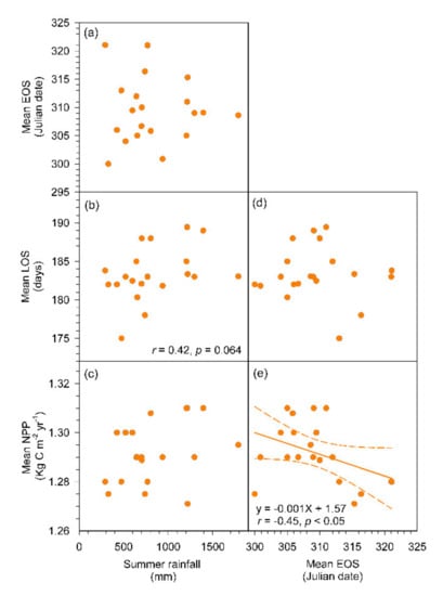
Figure 6.
The relationships between summer rainfall (August–October) and the mean EOS (a), mean LOS (b), and the mean NPP (c). Relationships between the mean EOS and the mean LOS (d), and mean NPP (e). The orange broken lines stand for 95% confident intervals, and the regression model is statistically significant with a p-value < 0.05.
3.3. Long-Term Variations of Vegetation Dynamics Related to Land Cover and Climatic Fluctuations
Based on the time series PV images during 2001–2020 of Taiwan, North Taiwan (N Taiwan), and South Taiwan (S Taiwan), there were four principal components selected which interpreted most variations (95.8–96.0%) of the original dataset were obtained, PC1 (93.9–94.8%), PC2 (1.0–1.2%), PC3 (0.4–0.2%), and PC4 (0.1–0.3%), respectively. The patterns after PC4 could not be identified with related variables excluded. The first two major components, PC1 and PC2, were associated with dominant land cover types on an island-wide scale. The PC1 image (eigenvector) reflected the vegetation coverage over time increased from flat plains to mountain regions (Figure 7a), which is comparable to land use maps (Figure 1c). The temporal loadings of PC1 showed positive values and stable seasonal cycles, minimum in spring (January–February) and maximum in summer (July–August), and the loadings strongly related to monthly PV of entire Taiwan, N Taiwan, and S Taiwan (r = 0.94–0.98, p < 0.01; Figure 7b) and monthly PV of forested regions (r = 0.91–0.96, p < 0.01). The PC2 image (eigenvector) presented positive values in plain areas and negative values in mountainous areas (Figure 8a), and its positive loadings time series reached a maximum in the summer with a drop in the preceding month, and the negative loadings spread from November to May (Figure 8b). The PC2 loadings significantly related to farmland monthly mean PV of entire Taiwan, N Taiwan, and S Taiwan (r = 0.78–0.91, p < 0.01; Figure 8b). In addition, both PC1 and PC2 temporal loadings exhibited a significant linear relationship to concurrent monthly temperature (R2 = 0.28–0.75, p < 0.01), and a log-linear relationship to one-month lagged of precipitation (R2 = 0.23–0.61, p < 0.01; Figure 7c and Figure 8c), which were consistent to the PV-climate analysis across vegetation types at monthly scale (Figure 3).
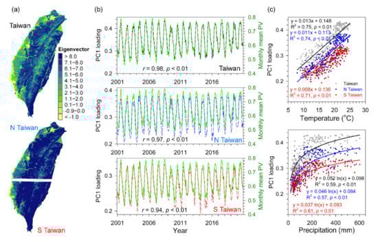
Figure 7.
The spatial eigenvectors of the first component (PC1) (a), temporal loadings and monthly mean PV obtained from the 2001–2020 monthly PV data (b), and the relationships between temporal loadings and temperature and precipitation (c) for entire Taiwan, North Taiwan (N Taiwan), and South Taiwan (S Taiwan).
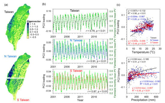
Figure 8.
The spatial eigenvectors of the second component (PC2) (a), temporal loadings and farmland monthly mean PV obtained from the 2001–2020 monthly PV data (b), and the relationships between temporal loadings and temperature and precipitation (c) for entire Taiwan, North Taiwan (N Taiwan), and South Taiwan (S Taiwan).
The third component (PC3) displayed positive eigenvector value in southwest Taiwan and lower altitudes, whereas the negative values major appeared in northeast Taiwan and higher elevations (Figure 9a), and its temporal loadings with dramatic variations were correlated to SPI3 for entire Taiwan (r = 0.40, p < 0.01), N Taiwan (r = 0.35, p < 0.01), and S Taiwan (r = 0.45, p < 0.01; Figure 9b). The fourth component (PC4) showed divergent patterns of positive and negative values in eastern and western Taiwan (Figure 10a), and the high positive loadings generally appeared during the highly negative SOI and negative loadings presented during higher positive SOI. There were significant negative correlations between loadings and SOI in entire Taiwan (r = –0.37, p < 0.05) and S Taiwan (r = –0.40, p < 0.05), but not in N Taiwan (r = 0.04, p = 0.69; Figure 10b).
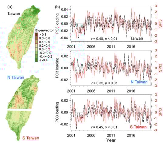
Figure 9.
The spatial eigenvectors of the third component (PC3) for entire Taiwan, North Taiwan (N Taiwan), and South Taiwan (S Taiwan) (a), and their temporal loadings and SPI3 (standardized precipitation index with a three-month time scale) (b).
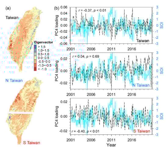
Figure 10.
The spatial eigenvectors of the fourth component (PC4) for entire Taiwan, North Taiwan (N Taiwan), and South Taiwan (S Taiwan) (a), and their temporal loadings and SOI (Southern Oscillation Index) (b).
4. Discussion
4.1. The Relationship between Vegetation Dynamics and Local Climate
The coefficients of determinations between PV and temperature (R2 = 0.35–75) are higher than the results between monthly PV and precipitation (R2 = 0.46–65) suggesting that the temperature plays a dominant control on vegetation growth with higher predictive power than precipitation based upon monthly time scale (Figure 3b,c). The R2s increase from forests to farmland and urban also reflect precipitation pattern decreasing from high altitudes to flat plain regions in which the vegetation in the lowland will be more sensitive to precipitation quantity (Figure 1b). Meanwhile, forests with well-developed roots than vegetation in farmland can utilize the soil moisture in-depth [91]. The linear relationships between monthly PV and concurrent temperature without time lag effects indicate that vegetation can develop promptly to the seasonal cycle of temperature, maximum in summer and minimum in winter. Studies showed that the favorable temperatures for vegetation growth are 6–30 °C in tropical and subtropical regions [92,93]. In Taiwan, even in winter, the monthly temperature in forested regions is rarely below 5 °C so that will not really limit plant growth (Figure 3b). However, the average of preceding one-month and concurrent month rainfall regulate the vegetation growth across various vegetation and land cover types (Figure 3c), demonstrating that the accumulation of precipitation amount especially for the winter–spring dry period plays a critical role to promoting vegetation activity during the transition time [94,95,96].
Previous studies have suggested that temperature is a major control on vegetation growth in temperate and boreal forests [5,6,11], while precipitation will significantly govern vegetation dynamics in arid and semi-arid regions [7,97,98]. The study conducted across various forest types in tropical and subtropical India revealed that the monthly mean NDVI related to concurrent monthly mean temperature, while the NDVI positive significantly correlated with the logarithm of preceding cumulative rainfall for 3–4 months [99]. Our findings exhibit that on a monthly scale, the linear relationships between temperature and PV without a time-lag effect across land cover types show the synchronous cycles of PV and temperature. However, the non-linear relationships between PV and precipitation with a one-month lag imply that the rainfall variations during the dry season have a substantial effect on the beginning of the growing season.
4.2. Spring and Summer Rainfall on Phenological Metrics
For the seasonal scale, the results show that the spring rainfall (February–March), but not summer rainfall (August–October), has a ramification on subsequent SOS, EOS, LOS, and NPP of Taiwan (Figure 5). The spatial patterns of later SOS (>JD 150) are associated with regions that received spring rainfall <40 mm, only 20% of the long-term average of the entire region, primarily distributed along central and southwestern Taiwan where it is most susceptible to drought effects [51]. Many studies in temperate forests and cold regions indicated that the land surface SOS is controlled by temperature, and plays a critical role in regulating ecosystem productivity [15,31,35,97]. In contrast, a recent study revealed that the relative contribution of EOS to LOS was higher than observed before [100]. In our results, the earlier SOS will bring about a longer growing season and increase productivity (Figure 5), but the negative correlation between EOS and NPP suggests that the delayed EOS is not favorable for vegetation production (Figure 6). Therefore, the impacts of rainfall accumulation during springtime and earlier SOS might lead to a cascade effect on vegetation activities, dynamics, and productivity of the annual cycle in subtropical Taiwan. Bigler et al. [101] found that water deficiency that occurred earlier in the growing period caused stronger effects on fir mortality than that happened late in the growing season or cessation (September to December). Over the past decade, the tropical ecosystems such as Congolese and Amazonia forests have experienced a large-scale reduction of vegetation greenness due to reduction in rainfall [10,102], in contrast, there was a widespread greening trend of vegetation in South Asia since 2002 owing to wetter conditions in the dry season or in the dry region [17]. The variations in vegetation dynamics indicated that the variations of carbon uptake and energy balance in tropics and subtropics are associated with rainfall anomalies.
In a global scale analysis over the last three decades (1981–2015), Famiglietti et al. [103] indicated that regions impacted by wet extremes are nearly as regions impacted by drought, in which the wet-impacted regions were not uniform in patterns controlled by multiple mechanisms. Knapp et al. [104] showed that aboveground net primary production was more responsive to soil moisture variability and increases in rainfall variability can rapidly change carbon cycling and vegetation composition, in lieu of changes in total precipitation. Under an era of a warming climate, the frequency and intensity of extreme hydro-climate events will increase and the variability of global carbon cycling and NPP will also be likely amplified [33,105,106,107,108]. In this study, the summer rainfall showed no statistically significant correlation to EOS and NPP, but the nearly significant relationship between summer rainfall and LOS (r = 0.42, p = 0.064) suggested that the effect will appear using a longer dataset or the climatic extremes such as tropical cyclone, sporadic rainfall storms in mountains, and other factors occurred within summer growing season should be considered in the future to disentangle the intertwined interactions on the vegetative surface.
4.3. Spatiotemporal Patterns of Vegetation Growth Associated with Land Surface Phenology and Climatic Fluctuations
The spatiotemporal patterns of the first two leading components of entire Taiwan, N Taiwan, and S Taiwan, as expected, were closely correlated to vegetation growth of land use, forests, and farmlands, respectively, and the temporal loadings were significantly related to local temperature and precipitation (Figure 7 and Figure 8). Unless the land surface has been dramatically altered over time, the constant land cover types interpreted the largest variability of vegetative greenness [47,109]. The higher eigenvectors in mountains of PC1 and stable seasonal cycles were associated with the vegetation growth for the entire island where was principally covered by forested regions in mid- and high-altitudes. In contrast, the higher eigenvector in plain regions of PC2 and the temporal loadings with an obvious drop during summer indicated that the regular interferences by anthropogenic forces such as irrigation or harvesting (Figure 8). Therefore, the combination of two images would be helpful for mapping the main land cover types, forest, and farmland (Figure 1c, Figure 7 and Figure 8).
The PC3 image was linked to regional drought conditions, where the annual precipitation declined from high altitudes and northeast Taiwan (negative eigenvectors) to lower altitude and southwest Taiwan (positive eigenvector) (Figure 9a). Over the 20-year period, there were similar positive-summer and negative-winter loadings which could characterize the seasonal climate in Taiwan, and the drought index SPI3 showed that during the period of 2002–2004 the negative loadings lasted for 27 months and was identified as the severest drought period over the past century, annual rainfall reached only 60% of long-term average [52] and might cause more significant impacts on S Taiwan than in N Taiwan (Figure 9b). Though climate warming might provide an upward trend in NPP, large-scale drought events would decrease NPP in that region and negate the benefit from increasing temperature such as in the tropical Amazon [110,111]. The records of climate over the last century manifested that the precipitation quantity tended to increase in northern Taiwan and to reduce in southern Taiwan, the fluctuations between wet and dry season has been intensified, and the projection of amplification will continue [112]. The exaggeration of drought conditions under warming scenarios is going to change hydroclimate, biogeochemical, and energy cycles, and the consequent disturbance on terrestrial ecosystems [113,114,115].
The PC4 revealed divergent eigenvector patterns of positive-eastern and negative-western that might be associated with rainfall anomalies and caused significant effects on S Taiwan than on N Taiwan (Figure 10b). The preceding warm events (El Niño) in the cold season over the Niño-3 region usually led to following wetter spring and wetter plum rainfall with frequent extreme events before summer in Taiwan, and vice versa [55,58]. Several studies using remotely sensed data showed that spatiotemporal patterns of the vegetative surface were connected with ENSO indicators which were linked to temperature in mid-latitude [43,116], rainfall variability, and flood in tropical Indonesia and the Amazon [49,50,117,118]. Our results showed that the patterns of the first three PCs were primarily controlled by local climatic factors, whereas the weak but substantial climatic signals associated with ENSO only can be captured by the low variance of vegetation using minor PC loadings (Figure 7, Figure 8, Figure 9 and Figure 10). Over the past three decades, the more intensive El Niño events in the central Pacific have become more common than the past four centuries, and the precipitation anomalies are also projected to shift eastward with the ongoing warming climate [119,120]. Recent studies reveal that ENSO phases have become a weaker factor over global-scale vegetation productivity than ever thought, but it is still a principal control of interannual variability of greenness over South America, northeastern Asia, eastern Australia, and southern and eastern Africa [121,122]. Therefore, it is urgent to disentangle the associations between vegetation dynamics and climatic fluctuation from regional to global scales, because the frequency and intensity of ENSO events continuously alter with climate warming.
4.4. Uncertainties and Perspective for Future Research
The monthly MVC PV images have decreased the atmospheric contamination significantly but there was approximately 1% of sampling points affected by unavoidable frequent clouds which could not completely eliminate the effect on the estimation of PV-climate relationships and land surface phenology. In PCA, the leading PCs usually could characterize the major patterns of land cover types, but there was no agreement between low order PCs and climatic anomalies which depended on region and time span of data used. It is always necessary to utilize longer data to comprehend the effects of regular climatic and climatic variations on the dynamics of vegetation growth in changing climates. Several studies suggested that CO2 fertilization and nitrogen deposition could enhance surface greenness [123,124], and it might be necessary to identify their contribution to vegetation dynamics but such data are not available across the mountainous island. The low cost of near-surface ground observation by WebCam or PhenoCam will be comparable in the near future for phenological observation across scale in selected sites [125], though the coverage of representative could be an issue in mountainous regions. The satellite-derived phenological information of vegetative surfaces is still the most powerful method for monitoring vegetation growth responses to changing climate across multiple spatiotemporal scales.
5. Conclusions
In this study, we synthesized the local climate, mainly temperature and precipitation, and large-scale ENSO anomalies, on vegetation dynamics in subtropical mountainous Taiwan using PV calculated from MODIS reflectance data to delineate vegetation growth at monthly, seasonal, and annual scales. The results indicate that PV is positively related to current monthly temperature and one-month lagged precipitation at a monthly timescale across various land cover types. The delayed SOS was directly influenced by a spring drought, <40 mm during February–March, and later SOS related to late EOS, shorter LOS, and reduction of annual NPP. However, the summer rainfall (August–October) and EOS were not significantly related to LOS and NPP. The SOS plays a critical role in controlling vegetation dynamics in this subtropical island. The PCA (principal component analysis) helped to effectively generate several patterns that accounted for most of the data variance and were associated with the phenology of land cover types (PC1 and PC2), regional drought condition (PC3), and large-scale atmospheric fluctuations (PC4). It is fundamental to disentangle the intertwined connections between vegetation and climate across multiple time scales that will be crucial for assessing the carbon sequestration and productivity of terrestrial ecosystems under the cascading effects of a specific climatic process in the near future.
Author Contributions
Software, data curation, formal analysis, writing—original draft, and writing—review and editing, H.-C.W.; conceptualization, methodology, supervision, software, data Curation, formal analysis, writing—original draft, and writing—review and editing, C.-T.C. All authors have read and agreed to the published version of the manuscript.
Funding
This research was funded by Ministry of Science and Technology, Taiwan (R.O.C.) to H.C.W. (Grant No. MOST 105-2621-B-845-001-MY2, 109-2313-B-845-001-) and C.T.C. (Grant No. MOST 105-2410-H-029-056-MY3, 108-2313-B-029-001-, 109-2621-B029-004- and 110-2313-B-029-002-).
Institutional Review Board Statement
Not applicable.
Informed Consent Statement
Not applicable.
Data Availability Statement
Not applicable.
Acknowledgments
We appreciate Cho-ying Huang at Department of Geography, National Taiwan University for his support of spectral mixture analysis. We also thank the anonymous reviewers for their constructive comments on earlier version of manuscript.
Conflicts of Interest
The authors declare no conflict of interest.
References
- Schimel, D.; Melillo, J.; Tian, H.; McGuire, A.D.; Kicklighter, D.; Kittel, T.; Rosenbloom, N.; Running, S.; Thornton, P.; Ojima, D.; et al. Contribution of increasing CO2 and climate to carbon storage by ecosystems in the United States. Science 2000, 287, 2004–2006. [Google Scholar] [CrossRef]
- Brando, P.M.; Balch, J.K.; Nepstad, D.C.; Morton, D.C.; Putz, F.E.; Coe, M.T.; Silvério, D.; Macedo, M.N.; Davidson, E.A.; Nóbrega, C.C.; et al. Abrupt increases in Amazonian tree mortality due to drought-fire interactions. Proc. Natl. Acad. Sci. USA 2008, 111, 6347–6352. [Google Scholar] [CrossRef] [PubMed]
- Sitch, S.; Friedlingstein, P.; Gruber, N.; Jones, S.D.; Murray-Tortarolo, G.; Ahlström, A.; Doney, S.C.; Graven, H.; Heinze, C.; Huntingford, C.; et al. Recent trends and drivers of regional sources and sinks of carbon dioxide. Biogeosciences 2015, 12, 653–679. [Google Scholar] [CrossRef]
- Myneni, R.B.; Keeling, C.D.; Tucker, C.J.; Asrar, G.; Nemani, R.R. Increased plant growth in the north high latitudes from 1981 to 1991. Nature 1997, 386, 698–702. [Google Scholar] [CrossRef]
- Nemani, R.R.; Keeling, C.D.; Hashimoto, H.; Jolly, W.M.; Piper, S.C.; Tucker, C.J.; Myneni, R.B.; Running, S.W. Climate-driven increases in global terrestrial net primary production from 1982 to 1999. Science 2003, 300, 1560–1563. [Google Scholar] [CrossRef] [PubMed]
- Suzuki, R.; Xu, J.Q.; Motoya, K. Global analyses of satellite-derived vegetation index related to climatological wetness and warmth. Int. J. Climatol. 2006, 26, 425–438. [Google Scholar] [CrossRef]
- Liu, Y.; Lei, H. Responses to natural vegetation dynamics to climate drivers in China from 1982 to 2011. Remote Sens. 2015, 7, 10243–10268. [Google Scholar] [CrossRef]
- Phillips, O.L.; Aragão, L.E.O.C.; Lewis, S.L.; Fisher, J.B.; Lloyd, J.; López-González, G.; Malhi, Y.; Monteagudo, A.; Peacock, J.; Quesada, C.A.; et al. Drought sensitivity of the Amazon rainforest. Science 2009, 323, 1344–1347. [Google Scholar] [CrossRef]
- Gond, V.; Fayolle, A.; Pennec, A.; Cornu, G.; Mayaux, P.; Camberlin, P.; Doumenge, C.; Fauvet, N.; Gourlet-Fleury, S. Vegetation structure and greenness in central Africa from Modis multi-temporal data. Philos. Trans. R. Soc. B Biol. Sci. 2013, 368, 20120309. [Google Scholar] [CrossRef] [PubMed]
- Hilker, T.; Lyapustin, A.I.; Tucker, C.J.; Hall, F.G.; Myneni, R.B.; Wang, Y.; Bi, J.; de Moura, Y.M.; Sellers, P.J. Vegetation dynamics and rainfall sensitivity of the Amazon. Proc. Natl. Acad. Sci. USA 2014, 111, 16041–16046. [Google Scholar] [CrossRef] [PubMed]
- Zhou, L.; Kaufmann, R.K.; Tian, Y.; Myneni, R.B.; Tucker, C.J. Relation between interannual variations in satellite measures of northern forest greenness and climate between 1982 and 1999. J. Geophys. Res. Atmos. 2003, 108, 4004. [Google Scholar] [CrossRef]
- Weigelt, P.; Jetz, W.; Kreft, H. Bioclimatic and physical characterization of the world’s island. Proc. Natl. Acad. Sci. USA 2013, 110, 15307–15312. [Google Scholar] [CrossRef]
- Moon, M.; Seyednasrollah, B.; Richardson, A.D.; Friedl, M.A. Using time series of MODIS land surface phenology to model temperature and photoperiod controls on spring greenup in North American deciduous forests. Remote Sens. Environ. 2021, 260, 112466. [Google Scholar] [CrossRef]
- Wenden, B.; Mariadassou, M.; Chielewski, F.M.; Vitasse, Y. Shifts in the temperature-sensitive periods for spring phenology in European beech and pedunculate oak clones across latitudes and over recent decades. Glob. Chang. Biol. 2020, 26, 1808–1819. [Google Scholar] [CrossRef]
- Wang, H.; Dai, J.; Zheng, J.; Ge, Q. Temperature sensitivity of plant phenology in temperate and subtropical regions of China from 1850 to 2009. Int. J. Climatol. 2015, 35, 913–922. [Google Scholar] [CrossRef]
- Bellón, B.; Bégué, A.; Lo Seen, D.; de Almeida, C.A.; Simõs, M. A remote sensing approach for regional-scale mapping of agricultural land-use systems based on NDVI time series. Remote Sens. 2017, 9, 600. [Google Scholar] [CrossRef]
- Wang, X.; Wang, T.; Liu, D.; Guo, H.; Huang, H.; Zhao, Y. Moisture-induced greening of the South Asia over the past three decades. Glob. Chang. Biol. 2017, 23, 4995–5005. [Google Scholar] [CrossRef] [PubMed]
- Zeng, L.; Wardlow, B.D.; Xiang, D.; Hu, S.; Li, D. A review of vegetation phenological metrics extraction using time-series, multispectral satellite data. Remote Sens. Environ. 2020, 237, 111511. [Google Scholar] [CrossRef]
- Botta, A.; Viovy, N.; Ciais, P.; Friedlingstein, P.; Monfray, P. A global prognostic scheme of leaf onset using satellite data. Glob. Chang. Biol. 2000, 6, 709–725. [Google Scholar] [CrossRef]
- Zhang, X.Y.; Friedl, M.A.; Schaad, C.B.; Strahler, A.H. Climate controls on vegetation phenological patterns in northern mid- and high latitudes inferred from MODIS data. Glob. Chang. Biol. 2004, 10, 1133–1145. [Google Scholar] [CrossRef]
- Rechid, D.; Raddatz, T.; Jacob, D. Parameterization of snow-free land surface albedo as a function of vegetation phenology based on MODIS data and applied in climate modelling. Theor. Appl. Climatol. 2009, 95, 245–255. [Google Scholar] [CrossRef]
- Kross, A.; Seaquist, J.W.; Roulet, N.T.; Fernandes, R.; Sonnentag, O. Estimating carbon dioxide exchange rates at contrasting northern peatlands using MODIS satellite data. Remote Sens. Environ. 2013, 137, 234–243. [Google Scholar] [CrossRef]
- Tang, X.; Li, H.; Griffis, T.J.; Xu, X.; Ding, Z.; Liu, G. Tracking ecosystem water use efficiency of cropland by exclusive use of MODIS EVI data. Remote Sens. 2015, 7, 11016–11035. [Google Scholar] [CrossRef]
- Ranghetti, L.; Bassano, B.; Bogliani, G.; Palmonari, A.; Formigoni, A.; Stendardi, L.; von Hardenberg, A. MODIS time series contribution for the estimation of nutritional properties of alpine grassland. Eur. J. Remote Sens. 2016, 49, 691–718. [Google Scholar] [CrossRef]
- Chang, C.T.; Wang, S.F.; Vadeboncoeur, M.A.; Lin, T.C. Relating vegetation dynamics to temperature and precipitation at monthly and annual timescales in Taiwan using MODIS vegetation indices. Int. J. Remote Sens. 2014, 35, 598–620. [Google Scholar] [CrossRef]
- Goward, S.N.; Prince, S.D. Transient effects of climate on vegetation dynamics satellite observations. J. Biogeogr. 1995, 22, 549–563. [Google Scholar] [CrossRef]
- Piao, S.L.; Fang, J.Y.; Zhou, Q.; Guo, M.; Henderson, M.; Ji, W.; Li, Y.; Tao, S. Interannual variations of monthly and seasonal normalized difference vegetation index (NDVI) in China from 1982 to 1999. J. Geophys. Res. 2003, 108, 4401. [Google Scholar] [CrossRef]
- Revadekar, J.V.; Tiwari, Y.K.; Kumar, K.R. Impact of climate variability on NDVI over the Indian region during 1981-2010. Int. J. Remote Sens. 2012, 33, 7132–7150. [Google Scholar] [CrossRef]
- Cleland, E.E.; Chuine, I.; Menzel, A.; Mooney, H.A.; Schwartze, M.D. Shifting plant phenology in response to global change. Trends Ecol. Evol. 2007, 22, 357–365. [Google Scholar] [CrossRef] [PubMed]
- Jeong, S.J.; Ho, C.H.; Gim, H.J.; Brown, M.E. Phenology shifts at start vs. end of growing season in temperate vegetation over the northern Hemisphere for the period 1982–2008. Glob. Chang. Biol. 2011, 17, 2385–2399. [Google Scholar] [CrossRef]
- Norman, S.P.; Hargrove, W.W.; Christie, W.M. Spring and autumn phenological variability across environment gradients of Great Smoky mountains National Park, USA. Remote Sens. 2017, 9, 407. [Google Scholar] [CrossRef]
- Menzel, A.; Sparks, T.H.; Estrella, N.; Koch, E.; Aasa, A.; Ahas, R.; Alm-Kübler, L.; Bissolli, P.; Braslavská, P.; Briege, A.; et al. European phenological response to climate change matches the warming pattern. Glob. Chang. Biol. 2006, 12, 1969–1976. [Google Scholar] [CrossRef]
- Breshears, D.D.; Cobb, N.S.; Rich, P.M.; Price, K.P.; Allen, C.D.; Balice, R.G.; Romme, W.H.; Kastens, J.H.; Floyd, M.L.; Belnap, J.; et al. Regional vegetation die-off response to global-change-type drought. Proc. Natl. Acad. Sci. USA 2005, 102, 15144–15148. [Google Scholar] [CrossRef]
- Qader, S.H.; Atikinson, P.M.; Dash, J. Spatiotemporal variation in the terrestrial vegetation phenology of Iraq and its relation with elevation. Int. J. Appl. Earth Obs. Geoinf. 2015, 41, 107–117. [Google Scholar] [CrossRef]
- Wang, H.; Tetzlaff, D.; Buttle, J.; Carey, S.K.; Laudon, H.; McNamara, J.P.; Spence, C.; Soulsby, C. Climate-phenology-hydrology interactions in northern high latitudes: Assessing the value of remote sensing data in catchment ecohydrological studies. Sci. Total Environ. 2019, 656, 19–28. [Google Scholar] [CrossRef]
- Zhao, J.; Zhang, H.; Zhang, Z.; Guo, X.; Li, X.; Chen, C. Spatial and temporal changes in vegetation phenology at middle and high latitudes of the Northern Hemisphere over the past three decades. Remote Sens. 2015, 7, 10973–10995. [Google Scholar] [CrossRef]
- Deng, H.; Yin, Y.; Wu, S.; Xu, X. Contrasting drought impacts on the start of phenological growing season in northern China during 1982–2015. Int. J. Climatol. 2020, 40, 3330–3347. [Google Scholar] [CrossRef]
- He, Z.; Du, J.; Chen, L.; Zhu, X.; Lin, P.; Zhao, M.; Fang, S. Impacts of recent climate extremes on spring phenology in arid-mountain ecosystems in China. Agric. For. Meteorol. 2018, 260–261, 31–40. [Google Scholar] [CrossRef]
- Li, X.; Fu, Y.H.; Chen, S.; Xiao, J.; Yin, G.; Li, X.; Zhang, X.; Geng, X.; Wu, Z.; Zhou, X.; et al. Increasing importance of precipitation in spring phenology with decreasing latitudes in subtropical forest area in China. Agric. For. Meteorol. 2021, 304, 108427. [Google Scholar] [CrossRef]
- Fu, Y.; Zhou, X.; Li, X.; Zhang, Y.; Geng, X.; Hao, F.; Zhang, X.; Hanninen, H.; Guo, Y.; De Boeck, H.J. Decreasing control of precipitation on grassland spring phenology in temperate China. Glob. Ecol. Biogeogr. 2021, 30, 490–499. [Google Scholar] [CrossRef]
- Philippon, N.; Martiny, N.; Camberlin, P.; Hoffman, M.T.; Gond, V. Timing and patterns of the ENSO signal in Africa over the last 30 years; insight from normalized difference vegetation index data. J. Clim. 2014, 27, 2509–2532. [Google Scholar] [CrossRef]
- Trenberth, K.E.; Dai, A.; van der Schrier, G.; Jones, P.D.; Barichivich, J.; Briffa, K.R.; Sheffield, J. Global warming and changes in drought. Nat. Clim. Chang. 2014, 4, 17–22. [Google Scholar] [CrossRef]
- Woodward, F.I.; Lomas, M.R.; Quaife, T. Global response of terrestrial productivity to contemporary climatic oscillations. Philos. Trans. R. Soc. B Biol. Sci. 2008, 363, 2779–2785. [Google Scholar] [CrossRef] [PubMed]
- Miyamoto, K.; Aiba, S.I.; Aoyagi, R.; Nilus, R. Effects of El Niño drought on tree mortality and growth across forest types at different elevations in Borneo. For. Ecol. Manag. 2021, 490, 119096. [Google Scholar] [CrossRef]
- Vicente-Serrano, S.M.; Grippa, M.; Delbart, N.; Le Toan, T.; Kergoat, L. Influence of seasonal pressure patterns on temporal variability of vegetation activity in central Siberia. Int. J. Climatol. 2006, 26, 303–331. [Google Scholar] [CrossRef]
- Chikoore, H.; Jury, M.R. Intraseasonal variability of satellite-derived rainfall and vegetation over Southern Africa. Earth Interact. 2010, 14, 1–26. [Google Scholar] [CrossRef]
- Mberego, S.; Sanga-Ngoie, K.; Kobayashi, S. Vegetation dynamics of Zimbabwe investigated using NOAA-AVHRR NDVI from 1982 to 2006: A principal component analysis. Int. J. Remote Sens. 2013, 34, 6764–6779. [Google Scholar] [CrossRef]
- Notaro, M.; Emmett, K.; O’Leary, D. Spatio-temporal variability in remotely sensed vegetation greenness across Yellowstone National Park. Remote Sens. 2019, 11, 798. [Google Scholar] [CrossRef]
- Gurgel, H.C.; Ferreira, N.J. Annual and interannual variability of NDVI in Brazil and its connections with climate. Int. J. Remote Sens. 2003, 24, 3595–3609. [Google Scholar] [CrossRef]
- Alessandri, A.; Navarra, A. On the coupling between vegetation and rainfall inter-annual anomalies: Possible contributions to seasonal rainfall predictability over land areas. Geophys. Res. Lett. 2008, 35, L02718. [Google Scholar] [CrossRef]
- Oliveira, L.M.T.; França, G.B.; Nicácio, R.M.; Antunes, M.A.H.; Cost, T.C.C.; Torres, A.R.; França, J.R.A. A study of the El Niño-Southern Oscillation influence on vegetation indices in Brazil using time series analysis from 1995 to 1999. Int. J. Remote Sens. 2010, 31, 423–437. [Google Scholar] [CrossRef]
- Chen, S.T.; Kuo, C.C.; Yu, P.S. Historical trends and variability of meteorological droughts in Taiwan. Hydrol. Sci. J. 2009, 54, 430–441. [Google Scholar] [CrossRef]
- Chang, C.T.; Wang, H.C.; Huang, C. Assessment of MODIS-derived indices (2001–2013) to drought across Taiwan’s forests. Int. J. Biometeorol. 2018, 62, 809–822. [Google Scholar] [CrossRef]
- Chen, J.M.; Fan, H.L. Interannual variability of the South China Sea summer rainfall and typhoon invading Taiwan. Atmos. Sci. 2003, 31, 221–238. [Google Scholar]
- Jiang, Z.H.; Chen, T.J.; Wu, M.C. Large-scale circulation patterns associated with heavy spring rain events over Taiwan in strong ENSO and non-ENSO year. Mon. Weather Rev. 2003, 131, 1769–1782. [Google Scholar] [CrossRef]
- Nagai, S.; Ichii, K.; Morimoto, H. Interannual variations in vegetation activities and climate variability caused by ENSO in tropical rainforests. Int. J. Remote Sens. 2007, 28, 1285–1297. [Google Scholar] [CrossRef]
- Brienen, R.J.W.; Phillips, O.L.; Feldpausch, T.R.; Gloor, E.; Baker, T.R.; Lloyd, J.; Lopez-Gonzalez, G.; Monteagudo-Mendoza, A.; Malhi, Y.; Lewis, S.L.; et al. Long-term decline of the Amazon carbon sink. Nature 2015, 519, 344–348. [Google Scholar] [CrossRef] [PubMed]
- Chang, C.T.; Wang, H.C.; Huang, C. Impacts of vegetation onset time on the net primary productivity in a mountainous island in Pacific Asia. Environ. Res. Lett. 2013, 8, 045030. [Google Scholar] [CrossRef]
- Huang, C.Y.; Chai, C.W.; Chang, C.M.; Huang, J.C.; Hu, K.T.; Lu, M.L.; Chung, Y.L. An integrated optical remote sensing system for environmental perturbation research. IEEE J. Sel. Top. Appl. Earth Obs. Remote Sens. 2013, 6, 2434–2444. [Google Scholar] [CrossRef]
- Asner, G.; Lobell, D. A biogeophysical approach for automated SWIR unmixing of soils and vegetation. Remote Sens. Environ. 2000, 74, 99–112. [Google Scholar] [CrossRef]
- Huete, A.; Didan, K.; Miura, T.; Rodriguez, E.P.; Gao, X.; Ferreira, L.G. Overview of the radiometric and biophysical performance of the MODIS vegetation indices. Remote Sens. Environ. 2002, 83, 195–213. [Google Scholar] [CrossRef]
- Yang, J.; Weisberg, P.J.; Bristow, N.A. Landsat remote sensing approaches for monitoring long-term tree cover dynamics in semi-arid woodlands: Comparison of vegetation indices and spectral mixture analysis. Remote Sens. Environ. 2012, 119, 62–71. [Google Scholar] [CrossRef]
- Abdi, H.; Seaquist, J.; Tenenbaum, D.; Eklundh, L.; Ardö, J. The supply and demand of net primary production in the Sahel. Environ. Res. Lett. 2014, 9, 094003. [Google Scholar] [CrossRef]
- Mora, C.; Caldwell, I.R.; Caldwell, J.M.; Fisher, M.R.; Genco, B.M.; Running, S.W. Suitable days for plant growth disappear under projected climate change: Potential human and biotic vulnerability. PLoS Biol. 2015, 13, e1002167. [Google Scholar] [CrossRef]
- Chiueh, P.T.; Shang, W.T.; Lo, S.L. An integrated risk management model for source water protection areas. Int. J. Environ. Res. Public Health 2013, 9, 3724–3739. [Google Scholar] [CrossRef]
- Muchoney, D.M.; Strahler, A.H. Pixel- and site-based calibration and validation methods for evaluating supervised classification of remotely sensed data. Remote Sens. Environ. 2002, 81, 290–299. [Google Scholar] [CrossRef]
- Chiu, C.A.; Lin, P.H.; Lu, K.C. GIS-based tests for quality control of meteorological data and spatial interpolation of climate data. Mt. Res. Dev. 2009, 29, 339–349. [Google Scholar] [CrossRef]
- Lana, X.; Serra, C.; Burgueño, A. Patterns of monthly rainfall shortage and excess in terms of the standardized precipitation index. Int. J. Climatol. 2001, 21, 1669–1691. [Google Scholar] [CrossRef]
- Lloyd-Hughes, B.; Saunders, M.A. A drought climatology for Europe. Int. J. Climatol. 2002, 22, 1571–1592. [Google Scholar] [CrossRef]
- Jin, Y.H.; Kawamura, A.; Jinno, K.; Berndtsson, R. Quantitative relationship between SOI and observed precipitation in southern Korea and Japan by nonparametric approaches. J. Hydrol. 2005, 301, 54–65. [Google Scholar] [CrossRef]
- Suppiah, R. Relationships between the Southern Oscillation and the rainfall of Sri Lanka. Int. J. Climatol. 1989, 9, 601–618. [Google Scholar] [CrossRef]
- Stone, R.; Auliciems, A. SOI phase relationships with rainfall in eastern Australia. Int. J. Climatol. 1992, 12, 625–636. [Google Scholar] [CrossRef]
- Plisnier, P.D.; Serneels, S.; Lambin, E.F. Impact of ENSO on East African ecosystems; a multivariate analysis based on climate and remote sensing data. Glob. Ecol. Biogeogr. 2000, 9, 481–497. [Google Scholar] [CrossRef]
- Jönsson, P.; Eklundh, L. TIMESAT—A program for analyzing time-series of satellite sensor data. Comput. Geosci. 2004, 30, 833–845. [Google Scholar] [CrossRef]
- Cong, N.; Wang, T.; Nan, H.J.; Ma, Y.C.; Wang, X.H.; Myneni, R.B. Changes in satellite-derived spring vegetation green-up date and its linkage to climate in China from 1982 to 2010: A multimethod analysis. Glob. Chang. Biol. 2013, 19, 881–891. [Google Scholar] [CrossRef]
- Suepa, T.; Qi, J.G.; Lawawirojwong, S.; Messina, P.J. Understanding spatio-temporal variation of vegetation phenology and rainfall seasonality in the monsoon Southeast Asia. Environ. Res. 2016, 147, 621–629. [Google Scholar] [CrossRef] [PubMed]
- Vivoy, N.; Arino, O.; Belward, A.S. The best index slope extraction (BISE): A method for reducing noise in NDVI time-series. Int. J. Remote Sens. 1992, 13, 1585–1590. [Google Scholar] [CrossRef]
- Moody, A.; Johnson, D.M. Land-surface phenologies from AVHRR using the discrete Fourier transform. Remote Sens. Environ. 2001, 75, 305–323. [Google Scholar] [CrossRef]
- Paruelo, J.M.; Lauenroth, W.K. Interannual variability of NDVI and its relationship to climate for North American shrublands and grasslands. J. Biogeogr. 1998, 25, 721–733. [Google Scholar] [CrossRef]
- Zhang, X.Y.; Friedl, M.A.; Schaaf, C.B.; Strahler, A.H.; Hodges, J.C.F.; Cao, F.; Reed, B.C.; Huete, A. Monitoring vegetation phenology using MODIS. Remote Sens. Environ. 2003, 84, 471–475. [Google Scholar] [CrossRef]
- Chen, J.; Jönsson, P.; Tamura, M.; Gu, Z.; Matsushita, B.; Eklundh, L. A simple method for reconstructing a high-quality NDVI time-series data based on Savitzky-Golay filter. Remote Sens. Environ. 2004, 91, 332–344. [Google Scholar] [CrossRef]
- Luo, Z.; Yu, S. Spatiotemporal variability of land surface phenology in China from 2001–2014. Remote Sens. 2017, 9, 65. [Google Scholar] [CrossRef]
- Cao, R.; Chen, Y.; Shen, M.; Chen, J.; Zhou, J.; Wang, C.; Yang, W. A simple method to improve the quality of NDVI time-series data by integrating spatiotemporal information with the Savitzky-Golay filter. Remote Sens. Environ. 2018, 217, 244–257. [Google Scholar] [CrossRef]
- Gao, F.; Morisette, J.T.; Wolfe, R.E.; Ederer, G.; Pedelty, J.; Masuoka, E.; Myneni, R.; Tan, B.; Nightingale, J. An algorithm to produce temporally and spatially continuously MODIS-LAI time series. IEEE Geosci. Remote Sens. Lett. 2008, 5, 60–64. [Google Scholar] [CrossRef]
- Chang, C.T.; Huang, C. Spatial patterns of vegetation phenology based on MODIS time-series data in Taiwan applying TIMESAT. J. Photogramm. Remote Sens. 2016, 20, 1–15. (In Chinese) [Google Scholar]
- Awange, J.; Hu, K.; Khaki, M. The newly merged satellite remotely sensed, gauge and reanalysis-based multi-source weighted-ensemble precipitation: Evaluation over Australia and Africa (1981–2016). Sci. Total Environ. 2019, 670, 448–465. [Google Scholar] [CrossRef]
- Saleem, A.; Awange, J.L.; Kuhn, M.; John, B.; Hu, K. Impacts of extreme climate on Australia’s green cover (2003–2018): A MODIS and mascon probe. Sci. Total Environ. 2021, 766, 142567. [Google Scholar] [CrossRef] [PubMed]
- Anyamba, A.; Eastman, J.R. Interannual variability of NDVI over Africa and its relation to El Niño/Southern Oscillation. Int. J. Remote Sens. 1996, 17, 2533–2548. [Google Scholar] [CrossRef]
- Lawley, E.F.; Lewis, M.M.; Ostendorf, B. Environmental zonation across the Australian arid region based on long-term vegetation dynamics. J. Arid Environ. 2011, 75, 576–585. [Google Scholar] [CrossRef][Green Version]
- Ali, L.; Reza, S.A. Statistical approach to determination of overhaul and maintenance cost of loading equipment in surface mining. Int. J. Min. Sci. Technol. 2013, 23, 441–446. [Google Scholar]
- Li, B.; Tao, S.; Dawson, R.W. Relations between AVHRR NDVI and ecoclimatic parameters in China. Int. J. Remote Sens. 2002, 23, 989–999. [Google Scholar] [CrossRef]
- Cunningham, S.; Read, J. Comparison of temperate and tropical rainforest tree species: Growth response to temperature. J. Biogeogr. 2003, 30, 143–153. [Google Scholar] [CrossRef]
- Queiroz, T.B.; Campoe, O.C.; Montes, C.R.; Alvares, C.A.; Cuartas, M.Z.; Guerrini, I.A. Temperature thresholds for Eucalyptus genotypes growth across tropical and subtropical ranges in South America. For. Ecol. Manag. 2020, 472, 118248. [Google Scholar] [CrossRef]
- Richard, Y.; Poccard, I. A statistical study of NDVI sensitivity to seasonal and interannual rainfall variations in Southern Africa. Int. J. Remote Sens. 1998, 19, 2907–2920. [Google Scholar] [CrossRef]
- De Beurs, K.M.; Henebry, G.M. Land surface phenology, climatic variation, and institutional change: Analyzing agricultural land cover change in Kazakhstan. Remote Sens. Environ. 2004, 89, 497–509. [Google Scholar] [CrossRef]
- Liu, X.; Zhu, X.; Li, S.; Liu, Y.; Pan, Y. Changes in growing season vegetation index and their associated driving forces in China during 2001–2012. Remote Sens. 2015, 7, 15517–15535. [Google Scholar] [CrossRef]
- Weiss, J.L.; Gutzler, D.S.; Coonrod, J.E.A.; Dahm, C. Long-term vegetation monitoring with NDVI in a diverse semi-arid setting, central New Mexico, USA. J. Arid Environ. 2004, 58, 249–272. [Google Scholar] [CrossRef]
- Shrestha, U.B.; Gautam, S.; Bawa, K.S. Widespread climate change in the Himalayas and associated changes in local ecosystems. PLoS ONE 2012, 7, e36741. [Google Scholar] [CrossRef]
- Prasad, V.K.; Badarinath, K.V.S.; Eaturu, A. Spatial patterns of vegetation phenology metrics and related climatic controls of eight contrasting forest types in India—Analysis from remote sensing datasets. Theor. Appl. Climatol. 2007, 89, 95–107. [Google Scholar] [CrossRef]
- Garrona, I.; De Jong, R.; De Wit, A.J.W.; Mucher, C.A.; Schmid, B.; Schaepman, M.E. Strong contribution of autumn phenology to changes in satellite-derived growing season length estimates across Europe (1982–2011). Glob. Chang. Biol. 2016, 20, 3457–3470. [Google Scholar] [CrossRef] [PubMed]
- Bigler, C.; Gavin, D.G.; Gunning, C.; Veblen, T.T. Drought induces lagged tree mortality in a subalpine forest in the Rock Mountains. Oikos 2007, 116, 1983–1994. [Google Scholar] [CrossRef]
- Zhou, L.; Tian, Y.; Myneni, R.B.; Ciais, P.; Saatchi, S.; Liu, Y.Y.; Piao, S.; Chen, H.; Vermote, E.F.; Song, C.; et al. Widespread decline of Congo rainforest greenness in the past decade. Nature 2014, 209, 86–90. [Google Scholar] [CrossRef]
- Famiglietti, C.A.; Michalak, A.M.; Konings, A.G. Extreme wet events as important as extreme dry events in controlling spatial patterns of vegetation greenness anomalies. Environ. Res. Lett. 2021, 16, 074014. [Google Scholar] [CrossRef]
- Knapp, A.K.; Fay, P.A.; Blair, J.M.; Collins, S.L.; Smith, M.D.; Carlisle, J.D.; Harper, C.W.; Danner, B.T.; Lett, M.S.; McCarron, J.K. Rainfall variability, carbon cycling, and plant species diversity in a mesic grassland. Science 2002, 298, 2202–2205. [Google Scholar] [CrossRef] [PubMed]
- Milly, P.C.D.; Dunne, K.A.; Vecchia, A.V. Global pattern of trends in streamflow and water availability in a changing climate. Nature 2005, 438, 347–350. [Google Scholar] [CrossRef] [PubMed]
- Kerr, R. The greenhouse is making the water-poor even poorer. Science 2012, 336, 405. [Google Scholar] [CrossRef] [PubMed]
- Seidl, R.; Thom, D.; Kautz, M.; Martin-Benito, D.; Peltoniemi, M.; Vacchiano, V.; Wild, J.; Ascoli, D.; Petr, M.; Honkaniemi, J.; et al. Forest disturbance under climate change. Nat. Clim. Chang. 2017, 7, 399–401. [Google Scholar] [CrossRef]
- Taufik, M.; Torfs, P.J.J.F.; Uijenhoet, R.; Jones, P.D.; Murdiyarso, D.; Van Lanen, A.J. Amplification of wildfire area burnt by hydrological drought in the humid tropics. Nat. Clim. Chang. 2017, 7, 428–432. [Google Scholar] [CrossRef]
- Lasaponara, R. On the use of principal component analysis (PCA) for evaluating interannual vegetation anomalies from SPOT/VEGETATION NDVI temporal series. Ecol. Model. 2006, 194, 429–434. [Google Scholar] [CrossRef]
- Zhao, M.; Running, S.W. Drought-induced reduction in global terrestrial net primary production from 2000 through 2009. Science 2010, 329, 940–943. [Google Scholar] [CrossRef]
- Lewis, S.L.; Brando, P.M.; Phillips, O.L.; van der Heijidenm, G.F.M.; Nepstad, D. The 2010 Amazon drought. Science 2011, 331, 5540. [Google Scholar] [CrossRef] [PubMed]
- Hsu, H.H.; Chen, C.T. Observed and projected climate change in Taiwan. Meteorol. Atmos. Phys. 2002, 79, 87–104. [Google Scholar] [CrossRef]
- Zeppel, M.J.B.; Wilks, J.V.; Lewis, J.D. Impacts of extreme precipitation and seasonal changes in precipitation on plants. Biogeosciences 2014, 11, 3083–3093. [Google Scholar] [CrossRef]
- Frank, D.; Reichstein, M.; Bahn, M.; Thonicke, K.; Frank, D.; Mahecha, M.D.; Smith, P.; van der Velde, M.; Vicca, S.; Babst, F.; et al. Effects of climate extremes on the terrestrial carbon cycle: Concepts, processes and potential future impacts. Glob. Chang. Biol. 2015, 21, 2861–2880. [Google Scholar] [CrossRef] [PubMed]
- Ummenhofer, C.; Meehl, G.A. Extreme weather and climate events with ecological relevance: A review. Philos. Trans. R. Soc. B Biol. Sci. 2017, 372, 20160135. [Google Scholar] [CrossRef]
- Park, K.A.; Bayarsaikhan, U.; Kim, K.R. Effects of El Niño on spring phenology of the highest mountain in north-east Asia. Int. J. Remote Sens. 2012, 33, 5268–5288. [Google Scholar] [CrossRef]
- Antico, A. Independent component analysis of MODIS-NDVI data in a large South American wetland. Remote Sens. Lett. 2012, 3, 383–392. [Google Scholar] [CrossRef]
- Arjasakusuma, S.; Yamaguchi, Y.; Hirano, Y.; Zhou, Y. ENSO- and rainfall-sensitive vegetation regions in Indonesia as identified from multi-sensor remote sensing data. ISPRS Int. J. Geo-Inf. 2018, 7, 103. [Google Scholar] [CrossRef]
- Freund, M.B.; Henley, B.J.; Karoly, D.J.; McGregor, H.V.; Abram, N.J.; Dommenget, D. Higher frequency of Central Pacific El Niño events in recent decades relative to past centuries. Nat. Geosci. 2019, 12, 450–455. [Google Scholar] [CrossRef]
- Yan, Z.; Wu, B.; Li, T.; Collins, M.; Clark, R.; Zhou, T.; Murphy, J.; Tan, G. Eastward shift and extension of ENSO-induced tropical precipitation anomalies under global warming. Sci. Adv. 2020, 6, eaax4177. [Google Scholar] [CrossRef] [PubMed]
- Gonsamo, A.; Chen, J.M.; Lombarodozzi, D. Global vegetation productivity response to climatic oscillations during the satellite era. Glob. Chang. Biol. 2016, 22, 3414–3426. [Google Scholar] [CrossRef]
- Zhao, L.; Dai, A.; Dong, B. Changes in global vegetation activity and its driving factors during 1982–2013. Agric. For. Meteorol. 2018, 249, 198–209. [Google Scholar] [CrossRef]
- Los, S.O. Analysis of trends in fused AVHRR and MODIS NDVI data for 1982-2006: Indication for a CO2 fertilization effect in global vegetation. Glob. Biogeochem. Cycles 2013, 27, 318–330. [Google Scholar] [CrossRef]
- Zhu, Z.; Piao, P.; Myneni, R.B.; Huang, M.; Zeng, Z.; Canadell, J.G.; Ciais, P.; Sitch, S.; Friedlingstein, P.; Arneth, A.; et al. Greening of the Earth and its drivers. Nat. Clim. Chang. 2016, 6, 791–795. [Google Scholar] [CrossRef]
- Richardson, A.D.; Hufkens, K.; Milliman, T.; Frolking, S. Intercomparison of phenological transition dates derived from the PhenoCam dataset V1.0 and MODIS satellite remote sensing. Sci. Rep. 2018, 8, 5679. [Google Scholar] [CrossRef]
Publisher’s Note: MDPI stays neutral with regard to jurisdictional claims in published maps and institutional affiliations. |
© 2021 by the authors. Licensee MDPI, Basel, Switzerland. This article is an open access article distributed under the terms and conditions of the Creative Commons Attribution (CC BY) license (https://creativecommons.org/licenses/by/4.0/).