Abstract
The parametric decomposition of full-waveform Lidar data is challenging when faced with heavy noise scenarios. In this paper, we report a fractional Fourier transform (FRFT)-based approach for accurate parametric decomposition of pulsed Lidar signals with noise corruption. In comparison with other joint time-frequency analysis (JTFA) techniques, FRFT is found to present a one-dimensional Lidar signal by a particular two-dimensional spectrum, which can exhibit the mathematical distribution of the multiple components in Lidar signals even with a heavy noise interference. A FRFT spectrum-processing solution with histogram clustering and moving LSM fitting is designed to extract the amplitude, time offset, and pulse width contained in the mathematical distribution. Extensive experimental results demonstrate that the proposed FRFT spectrum analysis method can remarkably outperform the conventional Levenberg–Marquardt-based method. In particular, it can accurately decompose the amplitudes, time offsets, and pulse widths of the pulsed Lidar signal with a −10-dB signal-to-noise-ratio by mean deviation ratios of 4.885%, 0.531%, and 7.802%, respectively.
1. Introduction
Pulsed light detection and ranging (Lidar) or laser altimetry is an important application of signal processing techniques in the field of laser remote sensing. Essentially, Lidar utilizes a time-of-flight (ToF) mechanism by projecting a laser on a target and capturing the echo signals backscattered from the entire surface of the target [1,2]. Subsequently, signal processing techniques are used to decompose the ToF, intensity, and other information from the pulsed Lidar signals, which are eventually used for geographic mapping. Currently, many signal processing techniques for parametric decomposition of full waveforms have been proposed and successfully applied, such as Levenberg–Marquardt (LM), Expectation-Maximum (EM), and B-spline algorithms [3,4,5,6,7,8,9,10,11]. However, almost all of these methods are discussed and tested on the Lidar waveforms in relatively high quality, without considering the heavy noise interference. In fact, laser beams are quite sensitive to environmental factors and optoelectronic systems during the long-distance remote sensing, which hampers the accuracy of these decomposition techniques. Although some approaches such as wavelet thresholding, empirical mode decomposition (EMD), and Kalman filtering have been used practically for denoising and enhancement of Lidar signals [8,9,10,12,13,14,15], they can only support the decomposition techniques to work well in a low-level noise condition. This is because the excessive filtering or denoising under a high-level noise condition will generate nonlinear distortion and residual noise, which still harms the stable and accurate parametric decomposition. To improve the detection range and accuracy in a noisy environment, more effective methods for parametric decomposition of pulsed Lidar signals with noise corruption are required.
One reason for the lack of robustness of the aforementioned methods to noise is that these methods work poorly in a single domain, namely either time domain or frequency domain. In terms of non-stationary signal processing, it is mostly insufficient to accurately analyze and process non-stationary signals in terms of a single domain, especially in a heavy noise scenario. Thus, a more effective solution called joint time-frequency localization (JTFL) or joint time-frequency analysis (JTFA) has been proposed and utilized to represent and analyze the non-stationary signals [16,17,18,19]. In principle, JTFA tracks the variations of a signal in time and frequency simultaneously and thereby constructs a two-dimensional (2D) time-frequency spectrum, which provides an overall and exhaustive description of the given signal. Thus, the JTFA techniques are superior to the conventional single-domain techniques in the anti-noise and positioning capabilities, which can facilitate the extraction of a weak signal from a strong noise environment and the decomposition of multiple components [20,21,22]. Some representative JTFA techniques, such as continuous wavelet transform (CWT), synchrosqueezing transform (SST), Wigner-Ville distribution (WVD), and fractional Fourier transform (FRFT), have been proposed for various applications, such as radar, acoustics, communication, and seismology [16,23,24,25,26,27,28,29]. The effectiveness is mainly attributed to the dedicated representation capabilities of these JTFA techniques for the signals with different characteristics. For example, FRFT and WVD can concentrate the energy of the chirp signals from radar, communications, or acoustics and both CWT and SST can represent a composite harmonic signal in seismology [30,31,32,33]. While these JTFA techniques have been tested successfully on these signals of different fields, there is a lack of the use of the JTFA technique for processing Lidar signals. A multi-pulse Lidar signal can be deemed a composite of multiple Gaussian components [34,35,36,37], which is largely different from a chirp or composite harmonic signal. Therefore, either the time variation or the frequency variation of a Lidar signal is continuous, infinite, and scattering, which makes these common JTFA techniques incompatible with Lidar signal analysis in the same way.
To overcome the difficulty of the application of JTFA to Lidar signal analysis and make use of the anti-noise capability of JTFA, we propose a FRFT spectrum analysis approach which outperforms the conventional single-domain technique for accurate parametric decomposition of pulsed Lidar signals with noise corruption. The remainder of this paper is organized as follows. In Section 2, we first review the theory of pulsed Lidar signals and state the requirements of parametric decomposition in a noisy environment. Then, the representative TFA techniques including CWT, SST, WVD, and FRFT are investigated and compared to present the advantage of FRFT in representation of pulsed Lidar signals. In Section 3, the FRFT representations of single-pulse and multi-pulse Lidar signals are mathematically deduced and verified to discover the the particular rules. In Section 4, a FRFT spectrum processing solution is designed for parametric decomposition under a noise condition based on the FRFT spectrum and its inherent rules. In Section 5, extensive experiments are carried out to display the entire operation process according to the previous theory and compare the performance of the proposed FRFT-spectrum method with the performance of the traditional LM-based methods under different noise conditions. Consequently, we validate the superiority of the proposed FRFT-spectrum method for accurate parametric decomposition of pulsed Lidar signals with noise corruption.
2. Related Work
2.1. Problem Formulation of Parametric Decomposition
Lidar possesses the capability of recording multi-pulse complete waveform of the backscattered signal echo; this approach was developed in 2004 to improve the detection efficiency and is called full-waveform Lidar [38]. Many full-waveform studies have been performed by employing the Gaussian model, which describes the Lidar waveforms as a sum of several Gaussian components [39,40,41]:
where K is the number of Gaussian components, the parameters represent the amplitude, ToF, and pulse width of the k-th Gaussian component, respectively. Accordingly, the multi-pulse Lidar aims to parameterize the signal via the parameters . Afterwards, the target characteristics including the reflectivity and range can be successfully derived and utilized for 3D imaging.
However, the actual echo signal acquired by the Lidar system suffers from variety of noise corruption. During laser propagation, the Lidar signal is subjected to various noise contaminations, such as atmospheric turbulence, atmospheric attenuation, target interaction, background solar noise, receiving electronic noise, etc. [42,43,44]. Overall, these noises can be classified into two types: multiplicative and additive noises; the multiplicative noise, i.e., the speckle noise, is manifested by randomly distributed dark and bright spots called speckle, which originates from random movement of atmospheric particles and random interactions of diffuse surfaces; the additive noise, i.e., the Gaussian noise, mainly comes from the receiving factors involving shot noise, amplifier noise, dark current noise, and background solar noise. As a consequence, the speckle noise broadens the Lidar pulse locally while the Gaussian noise has a global effect to bury the Lidar signal. Therefore, it becomes quite challenging to extract key parameters from the Lidar echo signal with strong additive noise. The difficulties are twofold. One issue is the effective extraction of the multi-pulse Lidar signals from the strong noise; the other issue is the accurate decomposition of all components and the attainment of characteristic parameters.
Traditional solution employs a one-dimensional (1D) signal processing technique to solve the two issues one by one. To address the first issue, some approaches were used for noise reduction, such as wavelet thresholding, EMD, and Kalman filtering. Wavelet thresholding is a multi-scale denoising technique, which has good characteristics of TF localization and outstanding performance in non-stationary signal processing. In particular, the wavelet thresholding technique removes the noise to the greatest extent while most of the details are preserved. Therefore, wavelet thresholding and related techniques have become very effective tools for Lidar signal denoising. Regarding the other issue on decomposition algorithms, the Levenberg–Marquardt (LM), Expectation-Maximum (EM), and B-spline algorithms are mostly used [3,4,5,6,7,8,9,10,11]. However, these algorithms greatly rely on the initial settings from the observed data and quite sensitive to the noise. When the Lidar echo signal is concealed in extremely strong noise, the combined technique of noise reduction and decomposition becomes useless. Therefore, it is significant to explore a better solution to decompose the parameters of the pulsed Lidar signals with strong noise corruption, which will be very useful for distant ranging and more accurate detection.
2.2. Exploration of Typical JTFA Techniques
As a 2D tool for signal analysis, the JTFA method has strong noise resistance and is widely used to extract weak signals from strong noise environments. However, due to the particularity of Lidar signals, no JTFA technique has ever been effectively used for parametric decomposition of pulsed Lidar signals. In this part, we explored the performances of the some representative JTFA methods including CWT, SST, WVD, and FRFT for Lidar signals. Theoretically, CWT has the characteristics of multi-resolution analysis compared with the traditional STFT and thus has the capability of localization in both the time and frequency domains [1,45]; SST improves the aggregation and resolution of TF distribution compared with CWT [2,30,46]; WVD is a bilinear transform (i.e., nonlinear transform) of the original signal to reach a high TF aggregation, which does not introduce any basis function like CWT and SST [23,47]; FRFT as a generalization of FT, rotates the original signal from the time domain to a generalized frequency domain by an arbitrary angle so as to track the overall distribution along the time and frequency domains [24,27,48,49].
To test the above four candidate JTFA techniques including CWT, SST, WVD, and FRFT, a simulation was implemented and the results are presented in Figure 1. The prior settings include: the laser pulse width is 20 ns; the time offset is 400 ns; the digitized rate is 1 GHz. Accordingly, pure 4-dB SNR and −10-dB SNR Lidar signals are simulated and shown in Figure 1(a1,b1,c1). Meanwhile, their CWT, SST, WVD, and FRFT spectra are shown in Figure 1(a2–a5,b2–b5,c2–c5) respectively. Overall, both the CWT and SST exhibit too much energy scattering for representation of pulsed Lidar signal while they generally are effective for representing the composition of discrete mono-harmonic components. With the increase of noise contamination, the CWT and SST spectra can hardly be recognized and extracted. Although WVD performs better than CWT and SST for the more focused energy, the shape of elliptical spectrum becomes deformed with increase of noise, thereby causing inaccurate parametric extraction. Furthermore, WVD will lead to cross items for multi-pulse Lidar signals due to its nonlinear property. In contrast to the previous three JTFA techniques, FRFT shows regular distribution even in a strong noise scenario, as shown in Figure 1(c5). Thus, the theoretical deduction and analysis are carried out in the following sections to verify the essential feasibility and efficiency for parametric decomposition of pulsed Lidar signals.
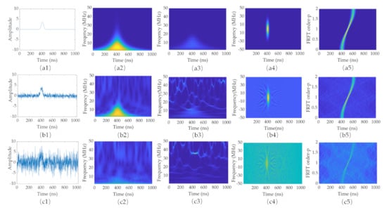
Figure 1.
(a1) Pure Lidar signal and its (a2) CWT, (a3) SST, (a4) WVD, and (a5) FRFT; (b1) noise-contaminated Lidar signal of 4 dB SNR and its (b2) CWT, (b3) SST, (b4) WVD, (b5) FRFT; (c1) noise-contaminated Lidar signal of −10 dB SNR and its (c2) CWT, (c3) SST, (c4) WVD, and (c5) FRFT.
3. FRFT Representation of Pulsed Lidar Signals
3.1. FRFT of Gaussian Kernel Function
FRFT was first proposed by Namias in 1980 to provide effective solutions for signal and image enhancement, restoration, recovery, and recognition, thus being widely used in areas of wave propagation, signal processing, and differential equations [28,29,48]. By introducing an angle parameter into the linear integral formula of FT, the p-order FRFT of a signal is defined as [24,27,48,49]:
where represents the kernel function of the FRFT, which is described as:
where , , n denotes an integer. According to the mathematical definition, some properties of the FRFT can be deduced. For brevity, only those useful to this study are listed as follows.
- (a)
- Time-shifting property:
- (b)
- Wigner distribution: The TF plane and all coordinates of the p-order FRFT are the results of rotating an angle relative to the original TF plane and the coordinates , which can be described as:
Mostly, FRFT is used for the processing of linear frequency modulated (LFM) signal namely the chirp signal, of which the WVD is a slash [50,51]. As per Equation (5), the slash is bound to be perpendicular to the u axis in the coordinates after a rotation of a certain angle , which means the FRFT result is converted to an impulse function. In other words, FRFT realizes the optimal focus of a single chirp signal at a certain angle and a certain u; thus, it can be used to accurate distinction and decomposition of a composite chirp signal even in a strong noise environment [26,52,53,54,55]. Different from the chirp signal, the WVD of a single Lidar signal is Gaussian, which means there is no possibility of converting the TF representation into an impulse function by rotation to reach the optimum focus. However, this does not mean there is no other effect of the FRFT on the Lidar signals to facilitate the extraction of the Lidar components from the strong noise.
Before exploring the FRFT of a multi-pulse Lidar signal which is universally represented by Equation (1), we first deduce the FRFT of a Gaussian basis function by substituting into Equation (2) and thus obtain the following result:
Overall, both the amplitude and the new incoming phase of the FRFT are Gaussian distributions of u. Specifically, when , the FRFT is converted into the FT of the Gaussian: . In fact, Equation (6) can be derived from the condition of with the time-shifting property of the FRFT represented by Equation (4). When , the FRFT of the Gaussian function is , which is no longer related to the order p. Essentially, the Wigner distribution plane of the Gaussian when is circular implies that the rotated plane always maintains the circular relationship. Consequently, the FRFT of the Gaussian along the p axis is uniform when .
3.2. FRFT Spectrum of Pulsed Lidar Signal
For a multi-pulse Lidar signal which contains multiple Gaussian components parameterized by , the FRFT of the k-th component can be derived according to the time shifting property in Equation (4):
where represents the modulus and the phase angle. To obtain , the items in Equation (6) are simplified as:
where and are respectively described by:
Here, we assume , where is the constant amplitude and is the Gaussian function of u. and are respectively expressed as:
Obviously, the pulse half-width of becomes:
Thus, the three conditions , , and are discussed as follows.
- (a)
- When : monotonically increases with the increase of within and decreases with the increase of within . When , reaches the maximum, which is . On the other hand, monotonically decreases with the increase of within and increases with the increase of within . When , reaches the minimum, which is . In summary, possesses the maximum amplitude and the minimum pulse width when .
- (b)
- When : monotonically decreases with the increase of within and increases with the increase of within . When , reaches the minimum, which is . On the other hand, monotonically increases with the increase of within and decreases with the increase of within . When , reaches the maximum, which is . In summary, possesses the minimum amplitude and the maximum pulse width when .
- (c)
- When : and do not vary with ,and remains .
The statements above indicate that the energy is more focused in the FRFT domain than the time domain when , less focused in the FRFT domain than the time domain when and remains unchanged when . To demonstrate the rules, simulations on Gaussian signals of = 2 ns, 0.5 ns and 1 ns are executed and their FRFT distributions are respectively shown in Figure 2a–c. Here, the ToF is assumed as .
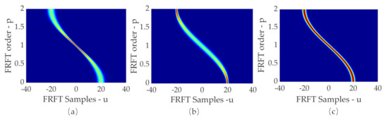
Figure 2.
FRFT distributions of signal-Gaussian signals of (a) , (b) and (c) .
Furthermore, Figure 2 indicates another characteristic with regard to symmetry. No matter which condition it is, the FRFT distribution within the plane is always centro-symmetric relative to a central point (0,1) since and ,that is:
It should be noted that, when the center of the time domain is not 0, the centro-symmetric point turns to be where is the central coordinate of the time domain. Moreover, is not an absolute number but a number related to the digitized rate. For instance, when the pulse width of Lidar signal is 1 ns and the sampling rate is 1 GHz, the FRFT distribution conforms to Condition (c). However, when the sampling rate is set to 2 GHz and 0.5 GHz respectively for the same Lidar signal of 1 ns, the FRFT distribution will transfer to Condition (a) and (c), respectively. Considering that the original sampling rate should satisfy the requirements of the Nyquist theorem for reliable recovery of Lidar pulses, the practical implementation only concentrates on Condition (a).
Based on the foregoing mathematical analysis of the FRFT of a single Gaussian signal and the linearity of the FRFT, the FRFT of a multi-pulse Lidar signal (i.e., multi-Gaussian signal) expressed by Equation (1) can be described by:
When , the offsets of all FRFT components are 0. In other words, the FRFT components overlap at point (0,1). Considering the foregoing corollary, we can draw the following conclusion: the FRFT distribution of a multi-pulse Lidar signal consists of multiple centro-symmetric spectral lines that intersect at the same point where is the central coordinate of the time domain. To test this point, a simulation is provided. The acquired data length is assumed to 4096 ns under a digitized rate of 1 GHz. The Lidar signal has three components, of which the ToFs are respectively = 1331 ns, = 2662 ns and = 3482 ns; the half-widths are respectively , and ; the amplitudes are respectively = 2.8 mV, = 3.6 mV and = 3.2 mV. After performing the FRFT on the Lidar signal, FRFT distribution of this signal over different values of p is presented in Figure 3. It is evident that the three centro-symmetric spectral lines intersect at the point where the energy is the most focused, which complies with the foregoing theoretical rule.
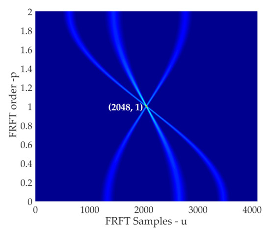
Figure 3.
Theoretical FRFT distribution of multi-pulse Lidar signal without noise.
4. FRFT Spectrum Processing Solution
In the previous sections, we found that the FRFT distribution is regularly recognizable even in strong noise situations and mathematically deduced the FRFT representation of a multi- pulse Lidar signal and summarized the distribution rule. Thus, the original problem of 1D time-domain signal processing is converted into the problem of 2D FRFT spectrum processing. In this section, we further investigate a solution of FRFT spectrum processing for accurate parametric decomposition.
The entire solution consists of three main steps. First, an image enhancement is employed to filter out the image noise and strengthen the components. Second, a ridge clustering method is used to determine the number of components and separate the ridges of the components. Finally, the feature extraction performs a fitting algorithm on the observed data of the separated ridges, finally obtaining ToFs, half-widths, and amplitudes of all components.
4.1. Enhancement of FRFT Spectrum
Image enhancement is a technique for removing as much noise as possible while preserving as many details as possible. To quantitatively evaluate the performance of the enhancement, we use the peak signal to noise ratio (PSNR) as an indicator, which is mathematically described by [56,57]:
For an 8-bit grayscale image, is 255. Considering that the observed image is not necessarily quantized to a gray level, is the peak intensity of the original image instead. In addition, in Equation (17) represents the mean square error (MSE) between the denoised image and the actual image and can be expressed as:
where is the image size (i.e., length × width) and and are respectively the filtered and original intensities of the pixel position .
Existing and effective image enhancement methods include mean filtering, median filtering, wavelet threshold filtering, Butterworth filtering, etc. Compared with median filtering, mean filtering is linear, which is more suitable to perform basic filtering on the noisy FRFT spectrum [58]. The output of pixel after mean filtering is:
where represents the weighted kernel function, which is actually a rectangle window with a size of , U and V are integers that satisfy and . The mean filter can result in a different filtering performance when is set differently. Generally, , which means the pixels within the windows are accumulated using the same weight.
Wavelet threshold filtering is a multi-scale denoising technique, which possesses good characteristics for TF localization [59,60,61], including hard thresholds and soft thresholds. Considering that the hard thresholds result in a high-frequency oscillation phenomenon (i.e., Gibbs phenomenon) and in a worse performance than soft thresholds, we choose to use the soft threshold filtering method in this study. There are many kinds of wavelet bases, and the number of wavelet layers can be freely selected. In practical application, we can combine them freely according to the specific situation.
To alleviate the edge loss and blurring produced by noise filtering, the Butterworth filter is further employed for image sharpening [62,63]. The system function of an n-order Butterworth high-pass filter is defined as follows:
where n represents the order of the filter, is the distance from the pixel position to the central position , and is a degree parameter. The greater is, the less high-frequency components of the image are reserved.
4.2. Clustering of Components and Extraction of ToFs
As shown in the flowchart in Figure 4, a stepwise processing of the enhanced FRFT spectrum is implemented as follows.
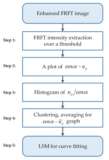
Figure 4.
Flowchart of ToF extraction approach.
Step 1: In order to filter out the useless noisy points, a local intensity image is extracted with layered thresholds, which are set as where is the mean value of the noise domain and is the standard deviation in a p-order condition.
Step 2: According to Equation (11), the FRFT peak intensity occurs at , which means the position of the peak intensity is linearly related to , we can draw a graph of according to this conclusion.
Step 3: After the slope of is obtained, we make mathematical statistics based on histograms. Essentially, the histogram is to equally divide the objective region into several intervals and record the frequency of the observed data within different interval. In this way, we can filter out some points that do not meet the requirements.
Step 4: Subsequently, automatic clustering is performed to determine the number of clusters and the corresponding points. The clustering algorithm consists of the following steps: (a) points with frequencies greater than a threshold are preserved and regarded as useful cluster points; (b) traverse all the cluster points: if the position of a current point is exactly adjacent to the position of a previous point, the current position is classified into the same cluster of the previous position; otherwise, the current position is classified into a new cluster; (c) Afterwards, traverse the next point and continue (b) until the last cluster point has been determined.
Step 5: After the clusters have been classified, the positions u of the different cluster points are averaged at different values of , which is defined as . Thus, the relationships between and can be obtained for different clusters.
Step 6: Using and , the ToFs of all components can be respectively derived by a curve-fitting algorithm. Here, the LSM is used to parameterize the observed data with and in the form of . Thus, we can obtain the fitting parameters by:
4.3. Extraction of Pulse Widths and Amplitudes
After the ToFs have been successfully extracted, the pulse width and amplitude require further exploration. According to Equations (12) and (13), we have two pieces of information available for obtaining the solution: one is the pulse distribution and the other is the peak intensity distribution . In contrast, the pulse-width information is more easily corrupted by a strong noise environment while the peak-intensity information is better preserved. Therefore, the latter solution is more reasonable and is thus adopted.
According to the foregoing mathematical relationship, we carry out the method shown in Figure 5 to extract the pulse widths and amplitudes of all components. It is vital that the employed FRFT-enhanced spectrum must be the linear image so that the intensity relationship will not be broken. Thus, we employ the mean-filtered FRFT spectrum for extraction of pulse widths and amplitudes. The entire procedure and the details of the steps are described as follows.
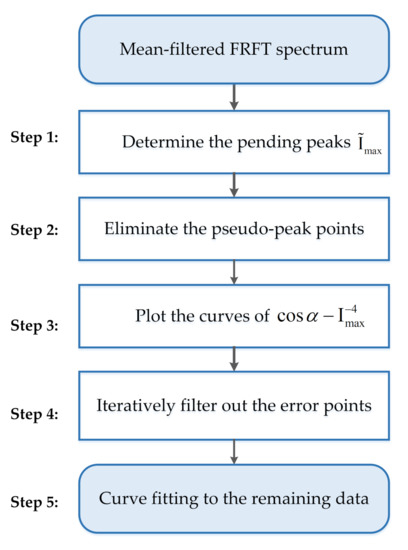
Figure 5.
Flowchart of pulse-width and amplitude extraction approach.
Step 1: Using the data in Figure 4 and the calculated results and , the pending peak intensities for different values of p are first determined by:
where represents the intensities of the enhanced FRFT spectrum and is a function of rounding a number to the nearest integer.
Step 2: Eliminate the pseudo-peak intensities from . In detail, go through all the at different values of , select a local interval centering on , and find the max intensity of the interval as . When is far less than , the at current is eliminated. Otherwise if approximates to , the at the current is preserved. After the elimination, the intensities of the remaining data are relabeled by .
Step 3: Plot the curve of with and explore the relationship between them. According to Equation (11), the curves should, in theory, approximate to a quadratic parabola. Using the effective peak intensities derived from Step (2), we finally obtain the curves of . When the error points of the observed data are not considered, we employ the fitting algorithm to determine the quantitative relationship between and , thus deriving the associated parameters. Considering the special relationships between , and in Equation (12), the quadratic polynomial formula should be specially set as . The LSM aims to find appropriate values of and to minimize the sum of squares of the deviations where are the observed peak intensities. Consequently, the parameters and are respectively determined by:
Thus, the half-pulse widths and amplitudes can be finally obtained by and . Considering that the current data contain many error points, curve fitting is not supposed to be used before the error points are eliminated.
Step 4: Error points near the center and on both sides of the curves are eliminated. On the one hand, as the central peak intensity is actually the intensity superimposed on the multiple compositions, it should not be used for any clusters. On the other hand, since the intensities of the two sides become relatively smaller as the deviations increase, they should also be ignored. Because the number of central error points is not very large, the former case is more easily handled. Generally, we may set a fixed threshold to filter out the points. The latter situation is more complicated since the degree of noise contamination differs for different clusters. To prune the observed points and determine the less-biased points for optimal fitting, an iterative algorithm is proposed as follows.
Algorithm:
- (a)
- The data length of is assumed to be L,a shifting step is initiated to 0.
- (b)
- Remove -point data simultaneously from two sides of the observed data. The length of the remaining data is reduced to . By using Equations (24) and (25), and are calculated, and the fitting curve is thus derived. The root-mean-square error (RMSE) between the remaining data and the fitting-curve data is obtained.
- (c)
- When the RMSE is less than a prescribed level or , the iteration ends; the calculated and are used for and ; otherwise, , continue Step (b).
It is noteworthy that the shifting scale of is not the shifting step but is expressed by where represents the shifting scale of .
5. Experimental Results
5.1. Data Acquisition
To investigate the real FRFT distribution of multi-pulsed Lidar signals in a strong noise scenario, we carried out an on-site experiment. The pulsed LIDAR system utilizes a 1064-nm solid laser with adjustable pulse width of 50∼80 ns. To determine the real ToF, amplitude, and width, we locate three calibration panels at three prescribed distances as the target surfaces and control the output power and pulse width of the laser emitter. By controlling the output power of the laser to an obviously low level ∼100 mW, weak pulsed Lidar signals are finally received by a linear-mode avalanche photodiode and digitized by a 1-GHz digitizer.
The full waveforms of Lidar signals can be recovered, as shown in Figure 6a. For comparison, the FT and CWT representations of the noisy signal are respectively derived and presented in Figure 6b,c. As can be seen from Figure 6a–c, the signals in the three domains of time, frequency, and wavelet are strongly concealed by heavy noise. The frequency spectrum, shown in Figure 6b, realizes good energy convergence of the three components but can hardly distinguish them. Although the wavelet spectrum shown in Figure 6c provides a TF view, it still cannot be used to part the components owing to scattering distributions of Gaussian components among the strong noises. In the absence of intuitive information, methods in Figure 6a–c can hardly realize accurate parameterization of the different components. According to the FRFT definition, we obtain the FRFT of the noisy signal and present it in Figure 6d. Different from the foregoing three types of signal representations, FRFT primarily retains the contours of the TF distribution, even with strong noise corruption.
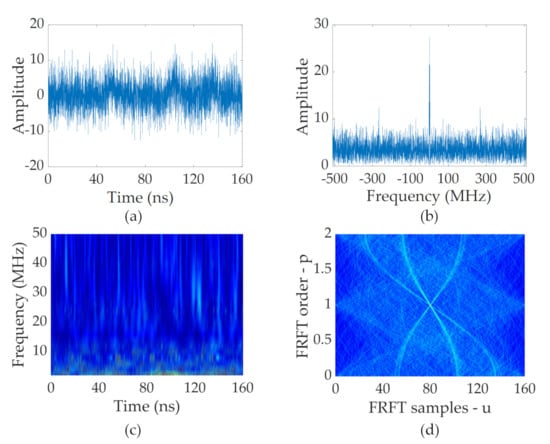
Figure 6.
(a) Noisy multi-pulse Lidar signals and its (b) FT, (c) CWT, and (d) FRFT.
5.2. Performance of FRFT Spectrum Enhancement
Based on the raw FRFT spectrum in Figure 6d, image enhancement is implemented. Figure 7a shows the result of mean filtering with a 5 × 5 kernel, of which the PSNR is 17.23 dB. As is shown, the details are effectively enhanced accompanied by broadening of the noise domain. Thus, the local noise still needs to be removed. To explore the optimal performance of soft-threshold wavelet filtering, the PSNRs of filtering results with different wavelet levels from 1 to 8 and bases from sym4, coief4, db2, to bior3.5 are tested and compared. As shown in Figure 8, it is evident that a higher level does not mean a better result. In fact, an increase in the wavelet level results in the removal of more details together with the noise, thus resulting in edge loss and image blurring. Here, the optimal denoising result occurs at the PSNR of 18.41 dB under a level of 5 and a base of sym4, which is displayed in Figure 7b.
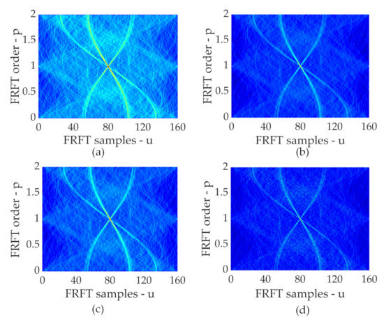
Figure 7.
Results of applying (a) mean filter, (b) wavelet-threshold filter, (c) both mean and wavelet-threshold filters, and (d) mean, wavelet-threshold, and Butterworth filters.
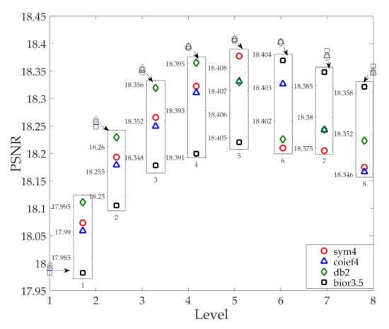
Figure 8.
PSNRs of soft-threshold wavelet filtering results with levels from 1 to 8 and bases of sym4 (marked by circle), coief4 (marked by triangle), db2 (marked by diamond), and bior3.5 (marked by square).
In order to utilize the attenuation property of the noise accumulation and the multiple shrinking of the wavelets, mean filtering and wavelet thresholding filtering are performed on the noisy image. Here, the optimal wavelet filtering with a basis of sym4 and a level of 5 is used. The kernel for the mean filtering remains at 5 × 5. By sequentially executing the mean and wavelet filtering, we obtain a further enhanced performance, as shown in Figure 7c. The PSNR is 18.82 dB, which is higher than the PSNR of using the separate techniques.
Although the combined method of the mean filter and wavelet thresholding filter effectively removes the noise, edge loss and image blurring occur. Thus, image sharpening should be further employed to improve the edges and eliminate the blurring. In the test, we set and for Butterworth filtering and derive the result shown in Figure 7d. Visually, the result has better clarity than Figure 7c. Quantitatively, the PSNR is 30.68 dB, which indicates a vast improvement compared with the non-sharpened result. To summarize the previous results, the PSNRs of the denoising results with different filtering methods are listed in Table 1. It is evident that the filtering method combining the mean, wavelet, and butterworth filters results in a particularly effective image enhancement of the FRFT spectrum, facilitating the subsequent parametric decomposition. The enhanced 2D FRFT spectrum exhibits much clearer global distribution of all components of pulsed Lidar signal.

Table 1.
The PSNRs of denoising results via different filters.
5.3. Performance of Parametric Decomposition
As mentioned before, the first step for parametric decomposition is to extract the ToFs from the enhanced spectral image. According to the solution given by Figure 3, we first filter the FRFT intensity image via layered thresholding and obtain the result shown in Figure 9a. Then, the changes in as a result of different values of are graphed in Figure 9b. The result of the statistical analysis contains three straight lines. To further remove the noisy points mixed in Figure 9b, only the points whose is greater than 1 or less than 4096 are preserved and used for histogram statistics. Here, the region of is divided to 160 times which means the resolution goes to 1 ns, and the histogram is shown in Figure 9c. After automatic clustering and equalization are performed, the graph of depicts the changes in (Figure 9d); different colors represent different clusters. Statistically, should approximate the peak positions of different orders. Visually, all the three clusters are linearly distributed. Finally, using the data in Figure 9d, we derive and of the three clusters and list them in Table 2. As the ToFs exist under the condition of , the peak positions of the different components are calculated by and thus listed in Table 2.
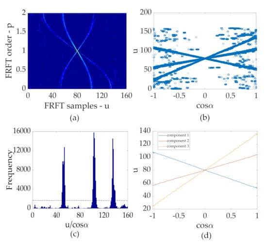
Figure 9.
(a) FRFT distribution over layered thresholds; (b) changes in of the observed data vs. ; (c) histogram of ; (d) changes in vs. after clustering and averaging.
Table 2.
The fitting results and the calculated ToFs regarding all clusters.
After obtaining the number of components and extracting the ToFs, pulse widths and amplitudes need to be further extracted. According to the solution given by Figure 10, pending peak intensities are determined and the pseudo-peak intensities are removed. Using the pruned peak intensities, the curve of with is plotted, as shown in Figure 10(a1,b1,c1).
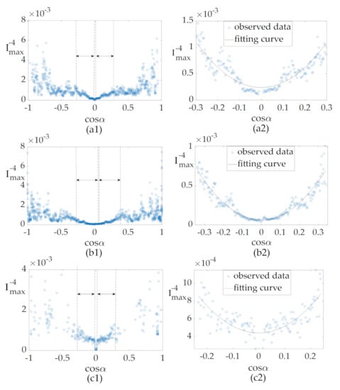
Figure 10.
Changes in vs. for (a1) Cluster 1, (b1) Cluster 2 and (c1) Cluster 3; fitting curves for observed data of (a2) Cluster 1, (b2) Cluster 2, and (c2) Cluster 3.
Obviously, the three distributions are visually consistent with the theoretical relationship. By using the curve fitting, the pulse widths and amplitudes can be finally obtained. However, the points on the both sides of these curves have great deviations and thus should be removed prior to curve fitting. To balance the tradeoff between more available points and less bias points, the iterative algorithm is used. Finally, we obtain the moving RMSEs of Clusters 1, 2, and 3 and plot the curves of and the RMSEs as shown in Figure 11. Here, we set and obtain the required for the three clusters of 0.700, 0.546, and 0.748 respectively. After eliminating the central error data, the useful data intervals are indicated by the double-headed arrows in Figure 10. Thus, the fitting results of the three clusters occurring at the required in the above algorithm are obtained and plotted in Figure 10(a2,b2,c2). Finally, the parameters of and are listed in Table 3.
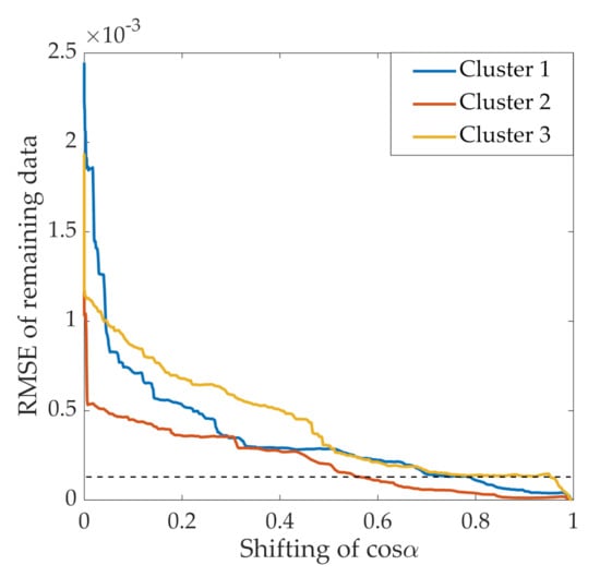
Figure 11.
Changes in the RMSE vs. the shifting scale from 0 to 1 for the three clusters.
Table 3.
The results of fitting parameters and the calculated pulse widths and amplitudes of all clusters.
For assessment, the RMSEs of the decomposed parameters regarding all clusters can be calculated as follows.
where C refers to the number of clusters; in the given experiment, . Moreover, and respectively refer to the decomposed and the real parameter values of the i-th cluster. Accordingly, the RMSEs of the amplitude, ToF, and pulse width obtained by the foregoing FRFT operation are 0.10, 11.84, and 2.05, respectively. For comparison, the most commonly used 1D signal processing method which combines denoising and nonlinear fitting are implemented. In detail, we employ the wavelet thresholding for noise reduction and the LM fitting algorithm for parametric decomposition, which is defined as WT-LM. Since the performance of Lidar signal denoising has great effect on the performance of parametric decomposition, different levels (i.e., level 1 to 8) and wavelet bases (i.e., sym4, sym8, db2 and bior3.5) are tested for noise reduction of the raw Lidar signal. By further use of LM fitting algorithm, the amplitudes, ToFs, and pulse widths of these denoised Lidar signals can be obtained. Thus, the RMSE variations of the three parameters with the increase of wavelet level are shown in Figure 12(a1,a2,a3), respectively. Overall, the proposed FRFT-spectrum method has remarkably better performance of parametric decomposition than the 1D signal processing method based on LM. In particular, the deviations of the pulse widths decomposed by all the candidate WT-LM methods are too large. Even the optimal pulse width decomposed by the WT-LM method with sym4 and level 6 has a deviation 24 times greater than the pulse width decomposed by the FRFT-spectrum method. To investigate the essence, the optimal LM fitting result from the corresponding wavelet denoised waveform (i.e., sym 4 and level 6) are shown in Figure 12b. In contrast to the amplitude and ToF, pulse width is more sensitive to the noise imposed on the real components, which is because the noise distributed on and around the real component easily leads to pulse widening after the denoising or smoothing operations. However, the denoising or smoothing techniques are very essential for the implementation of parametric decomposition in 1D signal processing. Therefore, the proposed FRFT-based approach can get rid of this tradeoff and achieve better parametric decomposition.
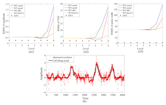
Figure 12.
Changes in RMSEs of (a1) amplitude, (a2) ToF and (a3) pulse width vs. wavelet level for different wavelet bases; (b) the WT-LM fitting result from the wavelet denoised waveform via sym4 and level 8.
To evaluate the performance of our proposed method under different SNRs, both the FRFT-spectrum and WT-LM methods are respectively performed on the simulated Lidar waveforms with SNRs varying from −10 dB to 10 dB. Thus, the mean deviations (MDs) of the three decomposed parameters from the real parameters can be respectively calculated by:
where and and C have the same meaning as those in Equation (26). Accordingly, the MDs of amplitudes, time offsets, and pulse widths under different SNRs are recorded and listed in Table 4, where the lower MDs are highlighted for each SNR to represent higher decomposition accuracy. Regarding the operation details, WT-LM requires initial parameter settings to activate the fitting process. In this simulation, we take [1; 2; 3], [1200; 2400; 3700], and [80; 80; 80] for initializations of amplitudes, time offsets, and pulse widths of three components, respectively. However, these appropriate initial settings can hardly be determined in low-SNR conditions without any prior knowledge, which greatly hinders feasible and accurate decomposition via such an iteration method. In contrast, the FRFT-spectrum method does not require exploring and specifying any initial parameters, which indicates a more direct and efficient operation. In terms of entire performance, the variations of WT-LM and FRFT-spectrum results in amplitude, time offset, and pulse width are shown in Figure 13. As illustrated by the red lines, the WT-LM method can reach satisfactory performance for parametric decomposition in a high SNR case, which is remarkably excellent in the decomposition of amplitude and time offset. However, when the SNR declines from −6 dB, the performance of FRFT drops dramatically. In contrast, the FRFT-spectrum method exhibits better performance in parametric decomposition than the WT-LM when SNR is less than −6 dB, as shown by the blue lines. In particular, the decomposition of pulse width via the FRFT-spectrum method is always far better than that via the WT-LM, as shown in Figure 13c. Essentially speaking, the heavy noise changes the direct distribution of time-domain signal hugely, thus greatly influencing accurate decomposition by the one-dimensional signal processing method. Meanwhile, the FRFT-spectrum expands the one-dimensional time or frequency domain to a two-dimensional time-frequency spectrum, which still presents real parametric distribution of Lidar signals statistically even in a rather low SNR situation. To summarize the above, our proposed FRFT-spectrum method can overcome the bottleneck of some one-dimensional signal processing methods and achieve excellent performance in parametric decomposition of pulsed Lidar signals under heavy noise scenarios.
Table 4.
Comparison of decomposition results between WT-LM and FRFT-S methods.
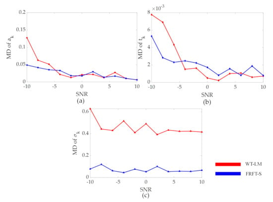
Figure 13.
Changes in MDs of (a) amplitude, (b) pulse width and (c) time offset vs. SNRs from −10 dB to 10 dB for WT-LM (in red) and FRFT-S (in blue) methods.
6. Discussion
The use of the FRFT for Lidar signals is essentially different from its conventional use for chirp signals. In terms of chirp signals, the FRFT aims to convert the original chirp form into an impulse form by rotating to a certain angle , thereby achieving the maximum energy convergence. Thus, the chirp parameters can be extracted with the specific theoretical relationship between the rotated angle and the parameters themselves. In a strict sense, the key point for chirp extraction lies in a certain angle where the transformed energy is more focused. In contrast, the Gaussian distribution of Lidar signals does not allow for achieving the most focused energy by rotation of a certain angle. However, the entire FRFT spectrum of Lidar signals presents particular characteristics. As deduced and tested before, the FRFT of a Gaussian component is a spectral line which is centro-symmetric to the angle . As for a pulsed Lidar signal, the FRFT spectrum exhibits multiple centro- symmetric spectral lines intersecting at the angle . These interesting characteristics explain why the FRFT can be applicable and efficient for pulsed Lidar signals even when the “most energy focus” principle cannot be applied.
Nevertheless, the present FRFT-spectrum approach only has remarkable performance for a coarse-grained Lidar detection from a long distance, such as detection by the airborne and satellite-borne systems. As for the fine-grained Lidar detection under which the pulse components of Lidar signals are heavily overlapped, our approach can only provide an average parametric measurement for different overlapped zones. Future studies will be devoted to finding a solution for this problem to enable a broader application of the proposed method.
7. Conclusions
This paper presented an FRFT-based approach for parametric decomposition of pulsed Lidar signals with strong noise corruption. To inspire the use of JTFA techniques for representation of pulse Lidar signals, some representative JTFA techniques including CWT, SST, WVD, and FRFT are investigated and compared. This preliminary trial indicates that FRFT distribution of pulsed Lidar signal is somewhat particular and quite robust to noise. Thus, we mathematically deduce the FRFT description of pulsed Lidar signals and find out the inherent rules. Based on the particular FRFT spectrums, we propose an FRFT spectrum processing solution which consists of image enhancement, auto-clustering, and feature extraction to realize the component parameterization. An onsite experiment is carried out to display the process of the foregoing theory. The final results demonstrate that the entire FRFT-based approach can achieve an accurate parametric decomposition of pulsed Lidar signals even in strong noise conditions, which is greatly superior to the traditional 1D signal processing approaches. Although the proposed FRFT-based approach can perform accurate decomposition on the component-separated Lidar waveforms for a coarse-grained Lidar detection, it can hardly distinguish the details of the component-overlapped Lidar waveforms for a fine-grained Lidar detection, which is a shortcoming expected to be overcome in future studies. To sum up, the principle, mechanism, and results reported in this paper can play an important role in improving the performance of many Lidar systems for robust remote sensing.
Author Contributions
Conceptualization, F.X.; methodology, F.X. and Q.W.; software, F.X. and J.C.; validation, F.X., J.C. and Y.L.; formal analysis, F.X. and Y.L.; investigation, J.C., Y.L. and Z.S.; resources, F.X., Q.W. and X.Z.; data curation, F.X. and J.C.; writing—original draft preparation, F.X.; writing—review and editing, F.X., J.C. and Y.L.; visualization, J.C. and Z.S.; supervision, F.X., Q.W. and X.Z.; project administration, F.X.; funding acquisition, F.X. All authors have read and agreed to the published version of the manuscript.
Funding
This work is supported by the National Natural Science Foundation of China (Grant No. 62001221), the China Postdoctoral Science Foundation Funded Project (Grant No. 2019M661830), the Jiangsu Planned Projects for Postdoctoral Research Funds (Grant No. 2021K087A), the Natural Science Foundation of Jiangsu Province, China (Grant No. BK20170813), and the Chinese Government Scholarship (Grant No. 201906835040).
Institutional Review Board Statement
Not applicable.
Informed Consent Statement
Not applicable.
Data Availability Statement
The data presented in this study are available on request from the corresponding author.
Acknowledgments
The authors would like to thank the editors and reviewers of this paper for their constructive suggestions.
Conflicts of Interest
The authors declare no conflict of interest.
References
- Altmann, Y.; Wallace, A.; McLaughlin, S. Spectral unmixing of multispectral lidar signals. IEEE Trans. Signal Process. 2015, 63, 5525–5534. [Google Scholar] [CrossRef]
- Groll, L.; Kapp, A. Effect of fast motion on range images acquired by lidar scanners for automotive applications. IEEE Trans. Signal Process. 2007, 55, 2945–2953. [Google Scholar] [CrossRef][Green Version]
- Hofton, M.A.; Minster, J.B.; Blair, J.B. Decomposition of laser altimeter waveforms. IEEE Trans. Geosci. Remote Sens. 2000, 38, 1989–1996. [Google Scholar] [CrossRef]
- Xu, F.; Li, F.; Wang, Y. Modified Levenberg–Marquardt-based optimization method for LiDAR waveform decomposition. IEEE Geosci. Remote Sens. Lett. 2016, 13, 530–534. [Google Scholar] [CrossRef]
- Qin, Y.; Li, B.; Niu, Z.; Huang, W.; Wang, C. Stepwise decomposition and relative radiometric normalization for small footprint LiDAR waveform. Sci. China Earth Sci. 2011, 54, 625–630. [Google Scholar] [CrossRef]
- Chauve, A.; Vega, C.; Durrieu, S.; Bretar, F.; Allouis, T.; Pierrot-Deseilligny, M.; Puech, W. Processing full-waveform lidar data in an alpine coniferous forest: Assessing terrain and tree height quality. Int. J. Remote Sens. 2009, 30, 5211–5228. [Google Scholar] [CrossRef]
- Reitberger, J.; Krzystek, P.; Stilla, U. Analysis of full waveform lidar data for tree species classification. Int. Arch. Photogramm. Remote Sens. Spat. Inf. Sci. 2006, 36, 228–233. [Google Scholar]
- Yan, S.; Yang, G.; Li, Q.; Wang, C. Waveform centroid discrimination of pulsed Lidar by combining EMD and intensity weighted method under low SNR conditions. Infrared Phys. Technol. 2020, 109, 103385. [Google Scholar] [CrossRef]
- Chang, J.; Zhu, L.; Li, H.; Xu, F.; Liu, B.; Yang, Z. Noise reduction in Lidar signal using correlation-based EMD combined with soft thresholding and roughness penalty. Opt. Commun. 2018, 407, 290–295. [Google Scholar] [CrossRef]
- Tian, P.; Cao, X.; Liang, J.; Zhang, L.; Yi, N.; Wang, L.; Cheng, X. Improved empirical mode decomposition based denoising method for lidar signals. Opt. Commun. 2014, 325, 54–59. [Google Scholar] [CrossRef]
- Shen, X.; Li, Q.Q.; Wu, G.; Zhu, J. Decomposition of LiDAR waveforms by B-spline-based modeling. ISPRS J. Photogramm. Remote Sens. 2017, 128, 182–191. [Google Scholar] [CrossRef]
- Zhou, Z.; Hua, D.; Wang, Y.; Yan, Q.; Li, S.; Li, Y.; Wang, H. Improvement of the signal to noise ratio of Lidar echo signal based on wavelet de-noising technique. Opt. Lasers Eng. 2013, 51, 961–966. [Google Scholar] [CrossRef]
- Zhang, Y.; Ma, X.; Hua, D.; Cui, Y.; Sui, L. An EMD-based denoising method for lidar signal. In Proceedings of the 2010 3rd International Congress on Image and Signal Processing, Yantai, China, 16–18 October 2010; Volume 8, pp. 4016–4019. [Google Scholar]
- Rocadenbosch, F.; Soriano, C.; Comerón, A.; Baldasano, J.M. Lidar inversion of atmospheric backscatter and extinction-to-backscatter ratios by use of a Kalman filter. Appl. Opt. 1999, 38, 3175–3189. [Google Scholar] [CrossRef] [PubMed]
- Sun, B.Y.; Huang, D.S.; Fang, H.T. Lidar signal denoising using least-squares support vector machine. IEEE Signal Process. Lett. 2005, 12, 101–104. [Google Scholar]
- Chen, V.C.; Ling, H. Joint time-frequency analysis for radar signal and image processing. IEEE Signal Process. Mag. 1999, 16, 81–93. [Google Scholar] [CrossRef]
- Kumar, R.; Zhao, W.; Singh, V. Joint time-frequency analysis of seismic signals: A critical review. Struct. Durab. Health Monit. 2018, 12, 65. [Google Scholar]
- Sharma, M.; Achuth, P.V.; Pachori, R.B.; Gadre, V.M. A parametrization technique to design joint time—Frequency optimized discrete-time biorthogonal wavelet bases. Signal Process. 2017, 135, 107–120. [Google Scholar] [CrossRef]
- Qian, S.; Chen, D. Joint time-frequency analysis. IEEE Signal Process. Mag. 1999, 16, 52–67. [Google Scholar] [CrossRef]
- Lao, G.; Yin, C.; Ye, W.; Sun, Y.; Li, G. A frequency domain extraction based adaptive joint time frequency decomposition method of the maneuvering target radar echo. Remote Sens. 2018, 10, 266. [Google Scholar] [CrossRef]
- Stanković, L.; Mandić, D.; Daković, M.; Brajović, M. Time-frequency decomposition of multivariate multicomponent signals. Signal Process. 2018, 142, 468–479. [Google Scholar] [CrossRef]
- Ahmad, A.A.; Lawan, S.; Ajiya, M.; Yusuf, Z.Y.; Bello, L.M. Extraction of the pulse width and pulse repetition period of linear FM radar signal using time-frequency analysis. J. Adv. Sci. Eng. 2020, 3, 1–8. [Google Scholar] [CrossRef]
- Daubechies, I. The wavelet transform, time-frequency localization and signal analysis. IEEE Trans. Inf. Theory 1990, 36, 961–1005. [Google Scholar] [CrossRef]
- Wang, P.; Gao, J.; Wang, Z. Time-frequency analysis of seismic data using synchrosqueezing transform. IEEE Geosci. Remote Sens. Lett. 2014, 11, 2042–2044. [Google Scholar] [CrossRef]
- Qian, S.; Chen, D. Decomposition of the Wigner-Ville distribution and time-frequency distribution series. IEEE Trans. Signal Process. 1994, 42, 2836–2842. [Google Scholar] [CrossRef]
- Almeida, L.B. The fractional Fourier transform and time-frequency representations. IEEE Trans. Signal Process. 1994, 42, 3084–3091. [Google Scholar] [CrossRef]
- Tant, K.M.; Mulholland, A.J.; Langer, M.; Gachagan, A. A fractional Fourier transform analysis of the scattering of ultrasonic waves. Proc. R. Soc. Math. Phys. Eng. Sci. 2015, 471, 20140958. [Google Scholar] [CrossRef] [PubMed]
- Weimann, S.; Perez-Leija, A.; Lebugle, M.; Keil, R.; Tichy, M.; Gräfe, M.; Heilmann, R.; Nolte, S.; Moya-Cessa, H.; Weihs, G. Implementation of quantum and classical discrete fractional Fourier transforms. Nat. Commun. 2016, 7, 1–8. [Google Scholar] [CrossRef] [PubMed]
- Saxena, R.; Singh, K. Fractional Fourier transform: A novel tool for signal processing. J. Indian Inst. Sci. 2005, 85, 11. [Google Scholar]
- Herrera, R.H.; Han, J.; van der Baan, M. Applications of the synchrosqueezing transform in seismic time-frequency analysis. Geophysics 2014, 79, V55–V64. [Google Scholar] [CrossRef]
- Ahrabian, A.; Looney, D.; Stanković, L.; Mandic, D.P. Synchrosqueezing-based time-frequency analysis of multivariate data. Signal Process. 2015, 106, 331–341. [Google Scholar] [CrossRef]
- Li, C.; Liang, M. A generalized synchrosqueezing transform for enhancing signal time–frequency representation. Signal Process. 2012, 92, 2264–2274. [Google Scholar] [CrossRef]
- Liu, W.; Cao, S.; Chen, Y. Seismic time–frequency analysis via empirical wavelet transform. IEEE Geosci. Remote Sens. Lett. 2015, 13, 28–32. [Google Scholar] [CrossRef]
- Galati, G.; Pavan, G.; De Palo, F. Chirp signals and noisy waveforms for solid-state surveillance radars. Aerospace 2017, 4, 15. [Google Scholar] [CrossRef]
- Sun, H.B.; Liu, G.S.; Gu, H.; Su, W.M. Application of the fractional Fourier transform to moving target detection in airborne SAR. IEEE Trans. Aerosp. Electron. Syst. 2002, 38, 1416–1424. [Google Scholar]
- Daubechies, I.; Lu, J.; Wu, H.T. Synchrosqueezed wavelet transforms: An empirical mode decomposition-like tool. Appl. Comput. Harmon. Anal. 2011, 30, 243–261. [Google Scholar] [CrossRef]
- Messioud, S.; Sbartai, B.; Dias, D. Harmonic seismic waves response of 3D rigid surface foundation on layer soil. Earthq. Struct. 2019, 16, 109–118. [Google Scholar]
- Mallet, C.; Bretar, F. Full-waveform topographic lidar: State-of-the-art. ISPRS J. Photogramm. Remote Sens. 2009, 64, 1–16. [Google Scholar] [CrossRef]
- Qin, Y.; Vu, T.T.; Ban, Y. Toward an optimal algorithm for LiDAR waveform decomposition. IEEE Geosci. Remote Sens. Lett. 2011, 9, 482–486. [Google Scholar] [CrossRef]
- Wagner, W.; Ullrich, A.; Ducic, V.; Melzer, T.; Studnicka, N. Gaussian decomposition and calibration of a novel small-footprint full-waveform digitising airborne laser scanner. ISPRS J. Photogramm. Remote Sens. 2006, 60, 100–112. [Google Scholar] [CrossRef]
- Qin, Y.; Vu, T.T.; Ban, Y.; Niu, Z. Range determination for generating point clouds from airborne small footprint LiDAR waveforms. Opt. Express 2012, 20, 25935–25947. [Google Scholar] [CrossRef] [PubMed]
- Steinvall, O.; Carlsson, T. Three-dimensional laser radar modeling. Proc. SPIE 2001, 4377, 23–34. [Google Scholar]
- Steinvall, O. Effects of target shape and reflection on laser radar cross sections. Appl. Opt. 2000, 39, 4381–4391. [Google Scholar] [CrossRef] [PubMed]
- Der, S.; Redman, B.; Chellappa, R. Simulation of error in optical radar range measurements. Appl. Opt. 1997, 36, 6869–6874. [Google Scholar] [CrossRef]
- Rioul, O.; Vetterli, M. Wavelets and signal processing. IEEE Signal Process. Mag. 1991, 8, 14–38. [Google Scholar] [CrossRef]
- Wang, S.; Chen, X.; Cai, G.; Chen, B.; Li, X.; He, Z. Matching demodulation transform and synchrosqueezing in time-frequency analysis. IEEE Trans. Signal Process. 2013, 62, 69–84. [Google Scholar] [CrossRef]
- Boashash, B.; Black, P. An efficient real-time implementation of the Wigner-Ville distribution. IEEE Trans. Acoust. Speech Signal Process. 1987, 35, 1611–1618. [Google Scholar] [CrossRef]
- Namias, V. The fractional order Fourier transform and its application to quantum mechanics. IMA J. Appl. Math. 1980, 25, 241–265. [Google Scholar] [CrossRef]
- Pei, S.C.; Ding, J.J. Fractional Fourier transform, Wigner distribution, and filter design for stationary and nonstationary random processes. IEEE Trans. Signal Process. 2010, 58, 4079–4092. [Google Scholar] [CrossRef]
- Lv, X.; Xing, M.; Zhang, S.; Bao, Z. Keystone transformation of the Wigner–Ville distribution for analysis of multicomponent LFM signals. Signal Process. 2009, 89, 791–806. [Google Scholar] [CrossRef]
- Barbarossa, S. Analysis of multicomponent LFM signals by a combined Wigner-Hough transform. IEEE Trans. Signal Process. 1995, 43, 1511–1515. [Google Scholar] [CrossRef]
- Alieva, T.; Bastiaans, M.J. On fractional Fourier transform moments. IEEE Signal Process. Lett. 2000, 7, 320–323. [Google Scholar] [CrossRef]
- Bastiaans, M.J.; Alieva, T.; Stankovic, L. On rotated time-frequency kernels. IEEE Signal Process. Lett. 2002, 9, 378–381. [Google Scholar] [CrossRef]
- Lohmann, A.W.; Soffer, B.H. Relationships between the Radon–Wigner and fractional Fourier transforms. JOSA A 1994, 11, 1798–1801. [Google Scholar] [CrossRef]
- Lohmann, A.W. Image rotation, Wigner rotation, and the fractional Fourier transform. JOSA A 1993, 10, 2181–2186. [Google Scholar] [CrossRef]
- Wu, H.R.; Yuen, M. A generalized block-edge impairment metric for video coding. IEEE Signal Process. Lett. 1997, 4, 317–320. [Google Scholar] [CrossRef]
- Zhou, W. Image quality assessment: From error measurement to structural similarity. IEEE Trans. Image Process. 2004, 13, 600–613. [Google Scholar]
- Kundu, A.; Mitra, S.; Vaidyanathan, P. Application of two-dimensional generalized mean filtering for removal of impulse noises from images. IEEE Trans. Acoust. Speech Signal Process. 1984, 32, 600–609. [Google Scholar] [CrossRef]
- Donoho, D.L.; Johnstone, I.M. Threshold selection for wavelet shrinkage of noisy data. In Proceedings of the 16th Annual International Conference of the IEEE Engineering in Medicine and Biology Society, Baltimore, MD, USA, 3–6 November 1994; Volume 1, pp. A24–A25. [Google Scholar]
- Donoho, D.L. De-noising by soft-thresholding. IEEE Trans. Inf. Theory 1995, 41, 613–627. [Google Scholar] [CrossRef]
- Chappalli, M.B.; Bose, N.K. Simultaneous noise filtering and super-resolution with second-generation wavelets. IEEE Signal Process. Lett. 2005, 12, 772–775. [Google Scholar] [CrossRef]
- Tang, H.Y.; Zhuang, T.G. Realizations of Fast 2D/3D Image Filtering and Enhancement. J. Shanghai Jiaotong Univ. (Sci.) 1998, 3, 108–112. [Google Scholar]
- Dogra, A.; Bhalla, P. Image sharpening by gaussian and butterworth high pass filter. Biomed. Pharmacol. J. 2014, 7, 707–713. [Google Scholar] [CrossRef]


Publisher’s Note: MDPI stays neutral with regard to jurisdictional claims in published maps and institutional affiliations. |
© 2021 by the authors. Licensee MDPI, Basel, Switzerland. This article is an open access article distributed under the terms and conditions of the Creative Commons Attribution (CC BY) license (https://creativecommons.org/licenses/by/4.0/).