Abstract
A series of marine remote sensing and ground-truth surveys were carried out at NW Gulf of Patras (W. Greece). The same area was surveyed in 1971 by Throckmorton, Edgerton and Yalouris, who are among the pioneers in the application of remote sensing techniques to underwater archaeology. The researchers conducted a surface reconnaissance survey to locate the site where the Battle of Lepanto took place on 7 October 1571. Their remote sensing surveying resulted in a map of two “target” areas that showed promise as possible remnants of wrecks from that battle and proposed a ground truth survey for their identification and in the detection of two modern shipwrecks. The ground truth survey was never fulfilled. The objectives of our repeat surveys, which were completed 50 years later, were to relocate the findings of this pioneer survey with higher spatial and vertical resolution, to ground-truth the targets, fulfilling their investigation, and to interpret the newly collected data in the light of modern developments in marine geosciences. Our repeat surveys detected mound clusters and individual mounds referred to “target” areas. These mounds could be interpreted as the surface expression of mud and fluid expulsion from the underlying deformed soft sediments. The ground truth survey demonstrated that the tops of mounds represent biogenic mounds. The ROV survey did not show any indication of wreck remnants of the Battle of Lepanto within the two survey areas. The site formation processes of the two modern shipwrecks were also studied in detail. Two noticeable seafloor morphological features were detected around the wreck sites; field of small-sized pockmarks and seafloor depressions. We would like to dedicate this work to the memory of Peter Throckmorton and Harold E. Edgerton, who are among the pioneers in the formative years of underwater archaeology in Greece.
1. Introduction
Around the late 1960s, the use of marine remote sensing techniques beyond the conventional diving methods (SCUBA) marked the beginning of a new era in maritime archaeology exploring shallow and deep-water depths and thus strengthening our knowledge of the ancient maritime world [1,2]. At these early stages, a significant remote sensing survey was carried out in Patras Gulf (western Greece) by Peter Throckmorton, a reporter–diver and a pioneer in underwater archaeology, and Harold E. Edgerton, professor of electrical engineering at M.I.T who developed side-scan sonar technology.
Prof. S. Marinatos—one of the premier Greek archaeologists of the 20th century who was the first to excavate the area of Akrotiri (Thera)—invited these researchers to search for the remains of the naval battle between the Christian and Ottoman fleets—the Battle of Lepanto. The researchers surveyed an area in the western part of the Patras Gulf, 10 km southeast of the island of Oxia (Figure 1a). They selected that area as the most possible site for the naval battle based on historical maps of the Gennadeion Library of the American School of Classical Studies in Athens, constructed in 1598, 1700 and 1702. At the time of the naval battle, 400 years ago, they assumed that the northern coastline of the Gulf of Patras at the mouth of the Acheloos river was located around 11 km north of the present location due to the large silting of the river.
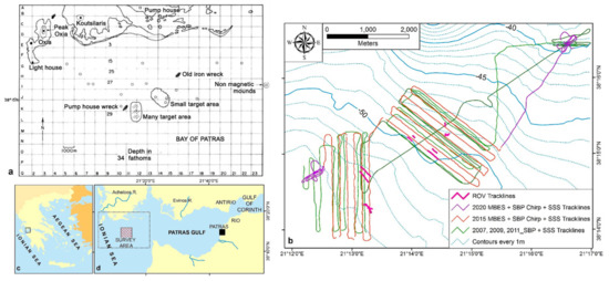
Figure 1.
(a) Map published by Throckmorton et al. (1973): (121, Figure 1) showing the “many target” and “small target” areas and the “pump house” and “old iron” wrecks. (b) Bathymetric map showing the 3.5 kHz, Chirp and side-scan sonar track lines and the R.O.V. transect in the survey areas at the western part of the Patras Gulf. (c,d) Sketch maps of Greece and Patras Gulf showing the study area (shaded rectangular) and the area corresponding to the map of Figure 1b.
Their survey was conducted over five cruises—four in 1971 and one in 1972—using the RV Stormie Seas. For the survey, the researchers employed all the available geophysical equipment of that time: (i) an EG and G side-scan sonar system covering the port side only, (ii) an EG and G penetrating pinger with a recorder Model 254 operating at a basic frequency of 5 kHz and a pulse length of 0.5 ms and (iii) an ELSEC Proton Magnetometer (Type 592). The navigation of the research vessel was based on several optical methods, and the accuracy of the worst-case position was ±400 m. The results of that survey were published in The International Journal of Nautical Archaeology and Underwater Exploration (1973), 2.1:121–130.
The side-scan sonar survey revealed the presence of numerous small targets, which appeared on the sonographs as shallow mounds, over an extensive area. Some targets were considered quite promising and were related to the remnants of the Battle of Lepanto, and a few others were considered interesting but of ambiguous origin. According to the authors, the shallow mounds could be associated with ancient wrecks or could be of geological origin. However, based on the areal distribution and the size of the targets, the researchers distinguished the studied area into two large areas defined as “many target” and “small target” areas (Figure 1a). Furthermore, the enhanced signal of the magnetometer over the “many target” area led the authors to conclude that this area was the most promising site of the remnants of the Battle of Lepanto and was the prime target for future investigation. In addition, the remote sensing survey discovered two steel wrecks. One of them was called a “pump house” wreck, as it was located approximately 9 km south of a local pump house, and the other was referred to as an “old iron” wreck (Figure 1a).
Although the survey resulted in a map of promising targets as possible sites of wrecks of the battle, the authors suggested that a visual inspection would be appropriate to identify the targets and confirm their origin. Unfortunately, that final step of the survey was never fulfilled. That innovative survey was the opening of a new era in archaeological oceanography in the Greek and eastern Mediterranean Sea, where the seafloor shelters the remains of glorious moments in prehistoric and historic times of the civilizations that developed on the surrounding coastline. A series of respective surveys would follow, attempting to investigate ancient and historic shipwrecks, naval battles and marine routes in Greek seas by using remote sensing techniques [3,4,5,6,7,8,9,10]. Over the last 15 years, marine remote sensing techniques have proven themselves in underwater archaeology predominately to be effective and reliable means of detecting ancient and historic shipwrecks and for site-specific archaeological surveys [11,12,13,14].
In the present work, we present the results of the new surveys, we compare the newly collected high resolution data with that of the initial study [15], and we interpret the new high-resolution data in the light of modern developments and aspects in geosciences and marine sciences. In this context, we have attempted to explore the relationship between sub-seabed soft-sediment deformation features and fluid expulsion and the presence of mounds that have been detected and mapped inside the two “target” areas of the original survey, using high-resolution sub-bottom profiling data. We also present the results of the ground truth survey of the mounds inside the two “target” areas retrieved after the interpretation of the geophysical data, thus fulfilling the unfinished survey of the pioneer researchers.
Moreover, we reveal the identity of the two initially detected unknown steel shipwrecks [15]. Finally, we study the site formation processes in the two shipwrecks from the point of view of the existence of soft sediments and fluid expulsion features in the area. Those two shipwrecks constitute one of the few well-documented examples of a possible causative relationship between pockmarks and shipwrecks.
2. Historical Environment
On 7 October 1571, two extraordinary fleets met at the entrance of the Gulf of Patras (known as Gulf of Lepanto at that time), and the battle that followed served to change the course of history. They were the fleet of the Holy League and the Ottoman fleet. In the battle that followed, the Holy League aimed for supremacy in the Mediterranean and to stop the territorial expansion of Ottomans in Europe. The Ottoman navy had become the greatest single naval power in the Mediterranean after 1538, capable of besieging Malta (1565), reaching the Caspian Sea (from 1569) and attacking Venetian-held Cyprus (1570) [16]. On the other hand, European forces (Spain, France, Italy) were distracted by their own issues, such as the dominance of Italy or Spanish affairs in territories far from the Mediterranean [17]. The Pope, through extensive negotiation, managed to overcome the internal divisions between the Christian states and to create the fleet of the Holy League, incorporating papal, Spanish, Venetian and Genoese fleets.
The Ottoman fleet numbered 230 warships commanded by Uluc Ali Pasha, and the Christian fleet numbered 208, commanded by Don Juan of Austria. The fleets comprised several types of galleys (gallia sottil, galiot, laternas, galleases, fustas) which carried flanking or centerline bronze guns [17]. An ordinary galley, which was the dominant warship of that battle, was 40 m long and 5 m wide. The vessel carried a centerline gun in its bow battery, flanked by two lighter pieces [17]. At the end of the battle, only 30 Ottoman galleys escaped; the rest was captured by the victors or sunk [16]. The Ottomans suffered over 30,000 dead and wounded and 3000 prisoners. The Christians lost 10 galleys and suffered 8000 men killed and 21,000 wounded. Among the allied wounded was Miguel de Cervantes, author of Don Quixote.
The battle was certainly a glorious victory for the allied navy, and Christian Europe was overwhelmingly joyful [16]. Famous paintings and frescoes in churches and palaces were created in memory of this battle. Beyond the immediate human and military consequences of this last major galley conflict, the Battle of Lepanto seemed to mark the passing of a new epoch in which the Mediterranean Sea no longer occupied a central position in the events that would mold the future of Europe [18].
4. Survey Design and Instrumentation
Forty kilometers of tracking remote sensing data were acquired over three three-day periods in September 2007, August 2009 and August 2011 (Figure 1b). Moreover, recurring marine remote sensing surveys were carried out in July 2015 and July 2020 using more advanced equipment (Figure 1b). The surveys covered a total area of 5.7 km2 centered on the “many target” area and the “small target” area as reported in [15] (Figure 1a). The extent of the western site, which is equivalent to the “many target” area, is 2.7 km2, and the extent of the eastern site, which is equivalent to the “small target” area, is 3.0 km2 (Figure 1b). Table 1 presents the various instrument characteristics against survey target analyses used in the original survey [15] and in each campaign of the present work.

Table 1.
Sensor device characteristics against survey target analyses for the original survey [15] and each campaign of the present work.
The surveys in 2007, 2009 and 2011 utilized (i) a dual-frequency hydrographic single beam echo sounder (Elac Nautic Hydrostar 4300), (ii) a dual-frequency (100 kHz and 500 kHz) EG and G 272 TD side-scan sonar tow fish in association with the EDGETECH 4200 Topside processor, (iii) a 3.5 kHz sub-bottom profiling system with a Geopulse transmitter and receiver (types 5430A and 5210A) and a 4 array transducer (type O.R.E. Ferranti 132B) in association with a Triton Imaging Inc digital recorder and (iv) a small light work-class R.O.V. (Benthos Minirover MKII) with a multicolor CCD camera and a 35 mm camera with flash. Positional data for the remote sensing and ground truth data, with a horizontal resolution of ±2 m, were provided by a Hemisphere GNSS with differential corrections. The navigation of the vessel was managed with the TritonMap software.
The surveys in 2007, 2009 and 2011 were organized in two phases. The first phase consisted of a systematic remote sensing survey of the seafloor using side-scan sonar and a high-resolution sub-bottom profiler. These two systems are commonly used in maritime archaeological surveys for the examination of seafloor morphology and stratigraphy and the detection of potential targets lying on the seafloor or buried in the sediments. In the present study, this instrumentation was additionally used to detect and relocate the targets reported in [15] (Figure 1b). The second phase incorporated a visual inspection at specific sites based on the results of the first phase (Figure 1b).
In July 2015 and 2020, repeat marine surveys took place using more advanced systems to gather data with a higher resolution compared to the previous surveys. The repeat surveys were conducted using (i) a Multibeam echosounder (MBES) Elak Nautik Seabeam 1185 with 300 m maximum operational depth, maximum swath coverage of 153° and the maximum number of sounding of 126 per swath, (ii) a “Chirp” Kongsberg Geoacoustics Geopulse Plus sub-bottom profiler system with a Universal transceiver, an acquisition display and an over-the-side Transducer Mounting (array of 4 transducers) with a hydrophone, (iii) an Edgetech dual Frequency (100 and 400 kHz) digital towfish 4200SP with an Edgetech 4200-P topside Processor and (iv) a Hemisphere Vector VS101 Compass GPS with two multipath resistant antennas with <0.5 m accuracy. The HYPACK software was used for the navigation of the vessel.
An 11 m long plastic-hull vessel (Irene, NP 464) was used for 2007, 2009 and 2011 surveys, and a 14 m long vessel (Milady Mylord III, ΝP 488) was used for the 2015 and 2020 surveys. The speed of both vessels was almost steady and ranged between 1.5 and 2 m/s. Both towfish were towed at a height of around 30 m above the seafloor at operational frequencies of 100 kHz, 400 kHz and 500 kHz. The range of each side-scan sonar lane was 100 m for each side (swath width of 200 m) and the lane spacing was 150 m, providing a 50% range overlap. Data were acquired without slant-range correction and were subsequently mosaiced using the Triton Imaging® Inc., Capitola, California, USA suite (Triton Isis and Tritonmap) software. The 3.5 kHz Geopulse sub-bottom profiler data were acquired using a 3.5 kHz frequency and a 1 ms pulse duration with a pulse rate of 10 s−1. The vertical resolution of the system was less than 0.5 m, which was the minimum distance between the distinguishable reflectors or targets. The Kongsberg Geopulse Plus sub-bottom profiler data were acquired using hyperbolic chirp (1.5–11.5 kHz) and Ricker pulses (3.3 and 4.6 kHz) with a pulse rate of 4 s−1 for a 32 ms chirp sweep. The “chirp” technology modifies the pulse as a range of frequencies are transmitted by the transducer, achieving more penetration and better resolution (~0.1 m). For the Elak Nautik Seabeam MBES survey, an SMC IMU-108 motion senor was used for pitch, roll and heave compensation with a resolution angle of 0.001° (pitch, roll) and resolution heave of 0.01 m. A hemisphere Vector VS101 GPS Compass with two multipath-resistant antennas and a heading accuracy of <0.10° rms was used for yaw compensation. A Sea&Sun Technology Sound Velocity Profiler with a resolution of 0.001 m/s and accuracy of ± 0.02 m/was used to collect the sound velocity profile. Both areas were sampled by close-range pulses (0–50°), offering a sample spacing ranging between 0.8 and 2.2 m per swath. According to the above, the point density could be estimated to an average of 1.5 points/m2.
5. Results and Discussion
5.1. Results of the Acquired Geophysical Data
High-resolution MBES bathymetric data highlight the presence of a smooth seafloor gently dipping to the southwest with an average gradient of 2°. The water depth over the survey area ranges from 38 to 54 m (Figure 2). Although the seafloor is generally flat, due to the high bathymetric point density and the data processing, it was possible to map the micro-relief (<0.5 m) at specific locations of the study area. The micro-relief of the seafloor consisted of small mounds and was mainly detected at the western part of the “many target” area and the south and south-western parts of the “small-target” area (Figure 2b).
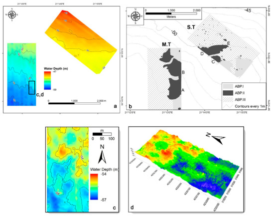
Figure 2.
(a) Bathymetric map of the two survey areas and location of Figure 2c,d. (b) Map showing the areal distribution of the three acoustic backscatter patterns in “many target” (M.T) and “small target” (S.T) areas deduced from the marine remote sensing survey (ABP.I: uniform soft seafloor, ABP.II: small mounds, ABP.III: long, linear to curvilinear features on the seafloor, A, B, C, D, E: mound clusters) (see also Figure 3 and Figure 4), (c) enlarged bathymetric map, and (d) enlarged 3D bathymetric map (location is shown in Figure 2a).
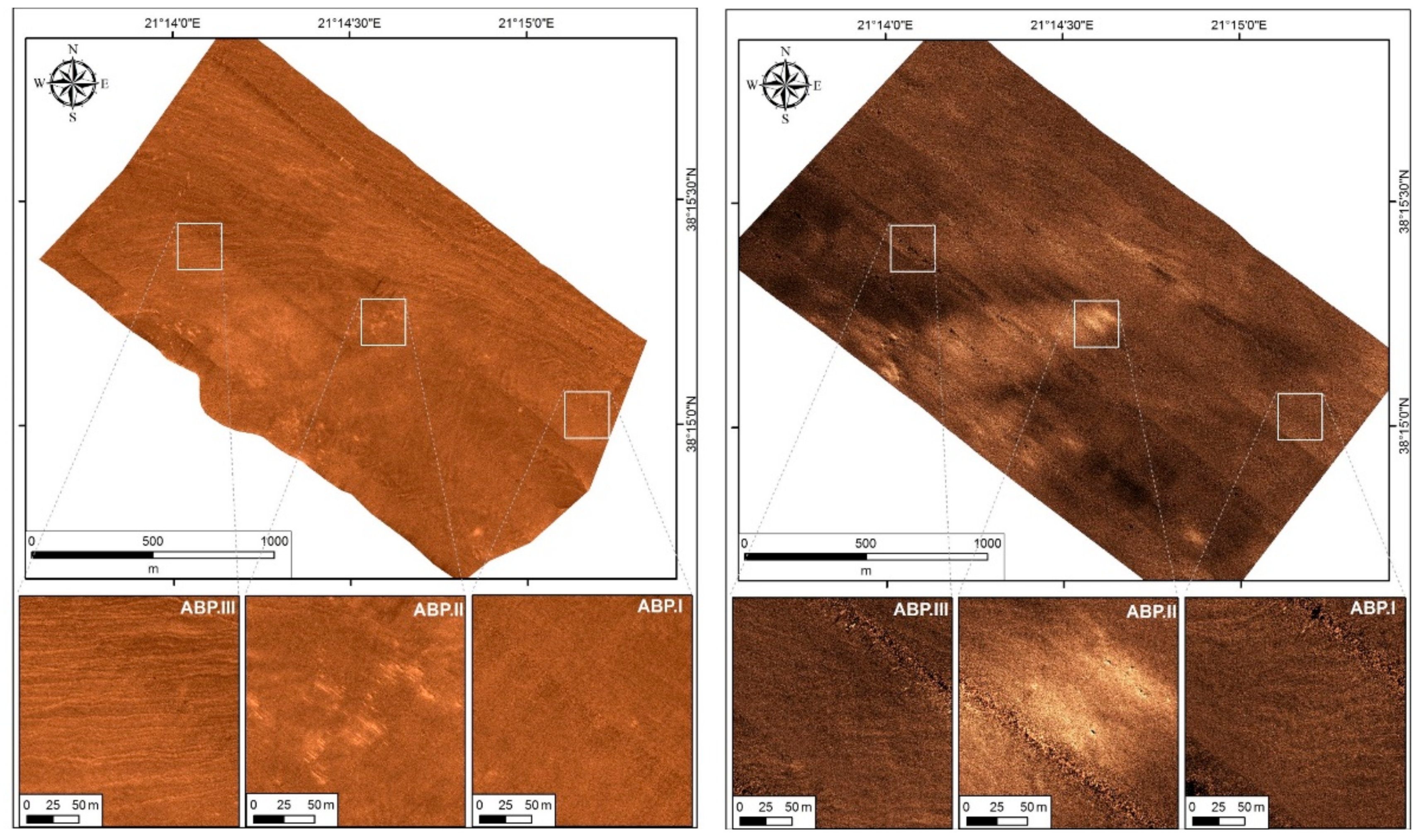
The interpretation of both the 100 kHz and 400 kHz side-scan sonar mosaics (Figure 3 and Figure 4) revealed three distinct acoustic backscatter patterns (ABP): (i) uniform low-reflectivity seafloor (ABP.I), (ii) localized strong backscatter facies in low reflectivity seafloor (ABP.II), an ABP that matches well with the micro-relief seafloor areas and (iii) numerous, long, linear to curvilinear and parallel to subparallel features on the seafloor (ABP.III) (Figure 2b).
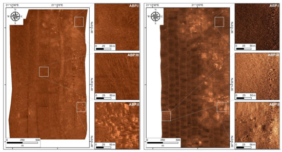
Figure 3.
Side-scan sonar mosaics at 100 kHz (left) and 400 kHz (right) of the “many target” area and representative sonographs of the three acoustic backscatter patterns.
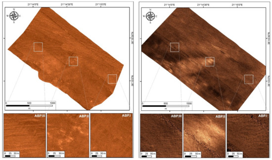
Figure 4.
Side-scan sonar mosaics at 100 kHz (left) and 400 kHz (right) of the “small target” area and representative sonographs of the three acoustic backscatter patterns.
Different types of seafloor produce a distinct return on the side-scan sonar records. The superficial sediment grain-size distribution, the seabed roughness, the epibenthic fauna and flora and gas-induced pockmarks strongly influence acoustic backscatter. In the digital sonographs presented in this study, lighter tones depict strong acoustic reflectivity and represent coarse-grained sediments that send back much more of the incident sound. Darker tones indicate seafloor areas that produce weak backscatter due to the presence of fine-grained sediments (mud and sand). The tone gradation in the analog side-scan sonar records is based on similar principles. In [15], the dark tones indicate strong reflectivity, and the light tones show weak reflectivity.
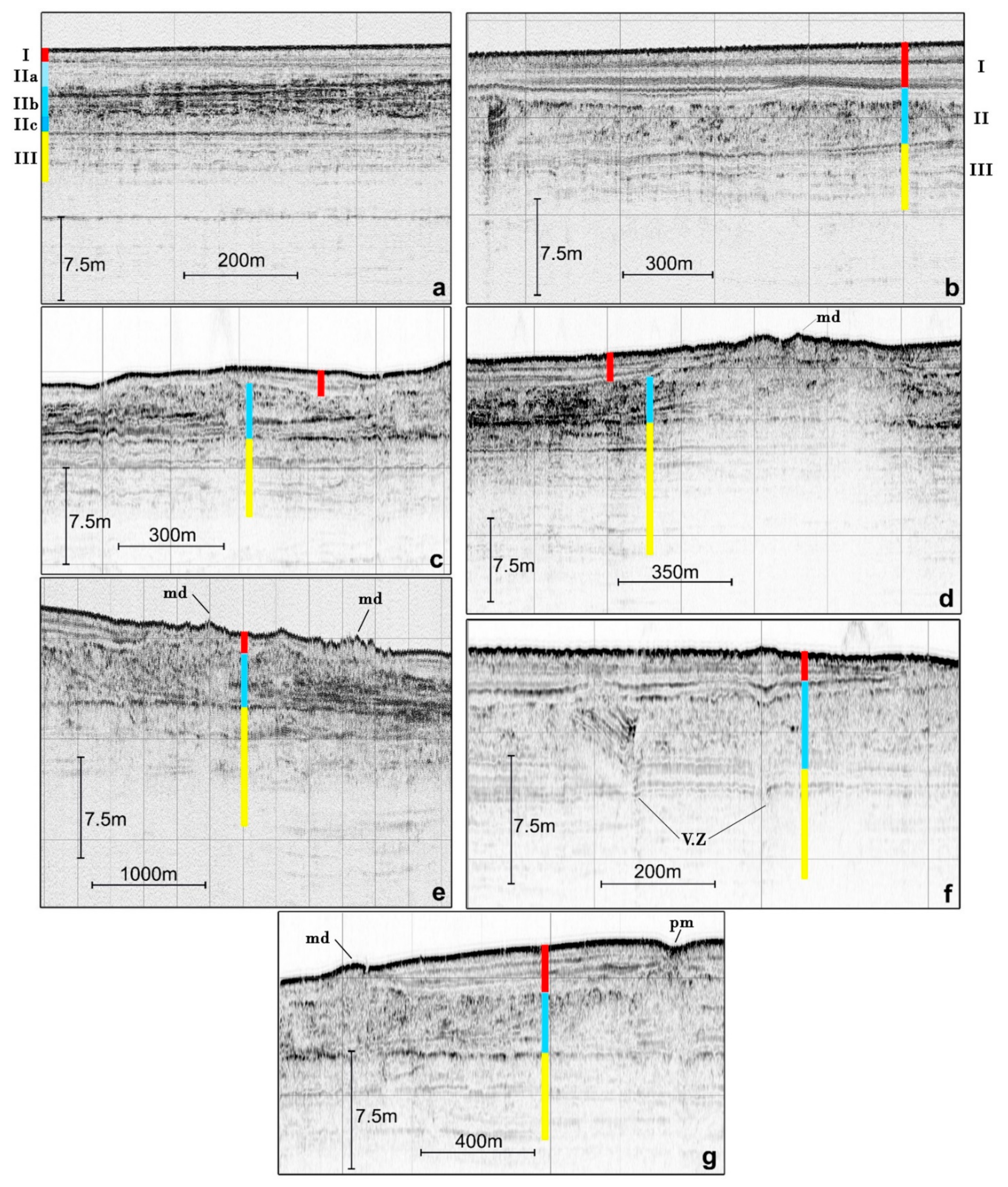
The 3.5 kHz and “chirp” profiles from the survey area showed that the seabed is characterized by three acoustic sequences (Figure 5a). The upper sequence (I) consists of parallel to subparallel reflectors overlying a high reflective–acoustic transparent sequence (sequence II) (Figure 5a). The topmost part of sequence II (IIa) is characterized by an acoustically semi-transparent layer with a few higher amplitude internal reflectors (Figure 5a).
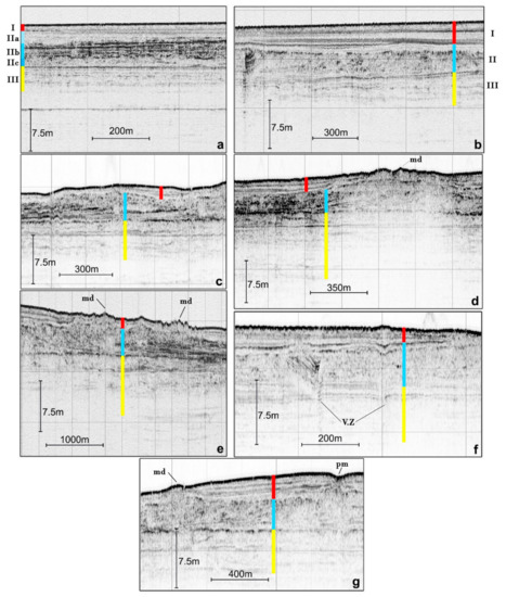
Figure 5.
Chirp seismic reflection profiles collected from the study area showing (a) specific acoustic characteristics of the three acoustic sequences (I, II, III). (b,c) The middle sequence II consists of a sediment body of chaotic seismic reflections with locally very disturbed reflectors and acoustic transparent zones, (d,e) sequence II locally subcrops and finally outcrops the seabed, forming small mounds (md), (f) vertical zones (vz) of seismic anomalies within the chaotic sequence II and the underlying III, and (g) negative (pockmarks? pm) and positive (mounds, md).
The middle part of sequence II (IIb) exhibits parallel to subparallel continuous high amplitude internal reflectors, while the base (IIc) is also characterized by an acoustically semi-transparent layer (Figure 5a). The lower sequence (III) consists of parallel strong to weak reflectors. The middle sequence (II), which has been observed as a composite well-shaped/acoustic transparent in the western part of the “many target” area, has been replaced, in the major part of the survey area, by a sediment body of chaotic seismic reflection appearance with locally very disturbed reflectors and acoustically transparent zones (Figure 5b). This chaotic deposit has a maximum thickness of 6 m and a more or less irregular top (Figure 5c). It seems that is composed of more than one stacked individual deposit, as indicated by the existence of seismic reflectors within the sediment body (Figure 5c,d). The deposit is covered by the sediments of sequence (I) but locally subcrops and finally outcrops the seafloor, forming small mounds (Figure 5d,e). These small mounds coincide well with the micro-relief area of the MBES data and the ABPII in the side-scan sonar mosaics. The internal acoustic character and the external shape characteristics suggest that this chaotic unit probably represents a deposit affected by soft-sediment deformation. Vertical zones of seismic anomalies were detected within the chaotic deposit and the underlying sequence (III) (Figure 5f). These features are characterized by down-bending marginal reflections and in some cases by an upward-convex reflector configuration towards their central zone (Figure 5f). These down-bending and upward-convex reflection signatures represent real structures rather than a sound velocity effect. Moreover, the features show clear evidence for seismic reflector truncations (Figure 5g). Based on the above characteristics, these features can be considered as vertical pore water and/or gas expulsions. In fluid expulsion features that terminate at the seafloor, negative (pockmarks?) and positive (mounds) have been observed and gas (?) flares have been also detected (Figure 5g).
The upward-convex reflector configuration within the fluid expulsion features may indicate sediment mobilization due to upward pore water and/or gas-enrichment fluid migration. Although the 3.5 kHz and chirp profiles, in the survey area, do not show the entire variety of acoustic characters of gas-charged sediments, the presence of gas within the sediment interstices of deeper sequences cannot be excluded. Disturbed and discontinuous reflectors of high reflectivity have been observed all over the survey area (Figure 6). The strong acoustic character of these reflectors can be attributed to the presence of gas within the sediment interstices (Figure 6). Furthermore, in studies presenting the seismic stratigraphy of the Patras Gulf [23,24,27,28], the authors suggested that the Pleistocene/Holocene boundary, 20–25 m beneath the seafloor, is a gas accumulative horizon, based on 3.5 kHz profiles selected from the eastern entire part of the Gulf.
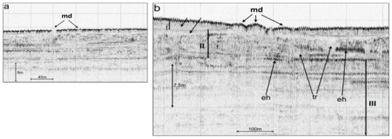
Figure 6.
Seismic reflection profiles at 3.5 kHz collected from the areas of mound clusters showing (a) examples of small mounds (coralligene algae reefs, md) over the soft seabed and (b) specific acoustic characteristics of the upper (I), middle (II) and lower (II) sequence. The middle (II) sequence has a complex internal geometry consisting of discontinuous and locally enhanced (eh) reflectors which are interrupted by areas of acoustically transparent facies (tr).
5.2. Coupling the Present Study and the Study of Thockmorton et al. (1973)
5.2.1. “Many Target” and “Small Target” Areas
The first acoustic backscatter pattern (ABP.I) on sonographs is characterized by uniform low-reflectivity (dark grey to black) and represents loose fine-grained superficial sediments (Figure 2b, Figure 3 and Figure 4). This pattern is in full agreement with the findings of [15], in which the seafloor was recorded with light tones on the sonographs indicating fine-grained sediments ([15]: 128, Figure 8; 129, Figure 9). The presence of a silty to sandy seafloor is further supported by the 3.5 kHz and chirp acoustic profiles.
The second acoustic backscatter pattern (ABP.II; Figure 2b, Figure 3 and Figure 4) in conjunction with the acquired 3.5 kHz and chirp profiles in the area represents small-scale mounds of low height (<1 m) (Figure 2b and Figure 3, Figure 4 and Figure 5). These mounds were detected as individuals but most commonly in dense clusters, forming a micro-relief seafloor and showing a similar acoustic signal to that of the targets described by [15] (Figure 3 and Figure 4).
The mound clusters and individual mounds detected in both survey areas are referred to as “many target” and “small target” areas by [15] (Figure 1). However, these two areas can be further distinguished based on the density in the occurrence of the clusters of the mounds and their acoustic backscatter characteristics.
The mound clusters have a higher density at the eastern part of the “many target” area (Figure 2b, Figure 3 and Figure 4). There, two extensive mound clusters (A and B) present densities ranging between 20 and 30 mounds/10−2km2 in occurrence (Figure 2b). In the “small target” area, the mounds are in three main clusters (C–E), but at lower densities ranging between 5 to 10 mounds/10−2km2 (Figure 2b). Moreover, the mounds 9j the “many target” areas present higher reflectivity and a sharper shape in relation to those obtained at the “small target” area (Figure 3 and Figure 4).
It seems that the above-mentioned differences in the density and acoustic signal between the mounds of the two areas explain the names proposed for them in [15]. Therefore, the western “many target” area is characterized by a significant number of well-shaped high reflectivity mounds and the eastern “small target” area is characterized by small mounds with lower reflectivity.
The 3.5 kHz and chirp seismic profiles, collected from the areas of mound clusters, provided further insight into the acoustic signature of these features (Figure 5d–g and Figure 6). The mounds appeared as hyperbolic and single dome-shaped, almost acoustically transparent structures (Figure 5d–g and Figure 6). The tops of the mounds are characterized by a low-amplitude acoustic signal that is always distinctly lower than that of the seafloor reflections from the adjacent areas (Figure 5d–g and Figure 6).
The seismic profiles have also shown that the chaotic deposit at the area of the small mounds exhibits a very complex internal acoustic character consisting of acoustically transparent and chaotic zones and discontinuous, locally land or seaward dipping, folded, and locally enhanced reflectors. The small mound areas are related to the chaotic deposit subcropping and outcropping at the seafloor. Therefore, the small mounds can be interpreted as the surface expression of mud and fluid expulsion from the underlying chaotic deposit. These mud and/or fluid expulsions rise through the surface sequence (I) due not only to the excess pore pressure induced by the deformation of the chaotic deposit but possibly due to gas-enrichment fluid migration.
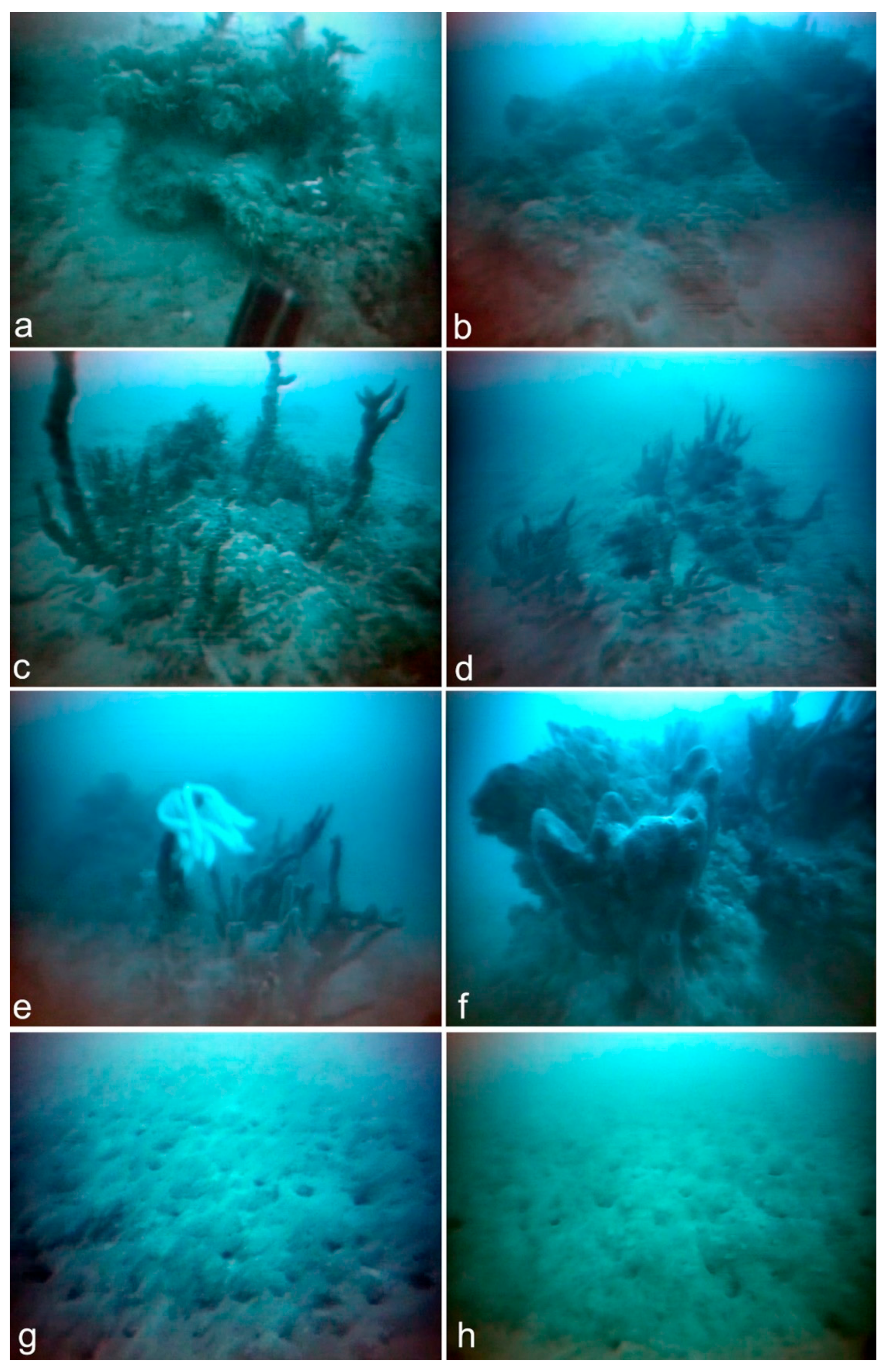
Several ROV dives were dedicated to examining the mounds in both survey areas (“many” and “small target”) (Figure 1b). The patchiness of the mounds’ appearance required large areas of the seafloor to be examined. Eventually, 11 ROV transects were conducted at both areas, covering a total linear distance of 2.9 km (Figure 1b). These transects were chosen to explore spatially the five detected mound clusters—two (A and B) were within the “many target” area and three (C–E) were in the “small target” area (Figure 2b). ROV dive transects demonstrated that the high-reflectivity mounds represent biogenic mounds (Figure 7). These mounds consist of calcareous small blocks which form a mound-like structure with a distinct positive relief (0.5–1.0 m) (Figure 7a,b). Small sponges, polychaetes and soft-tissue corals cover the top of the mounds (Figure 7c–f).

Figure 7.
R.O.V. photos showing (a,b) coralligene algae reefs less than 1.0 m in height, (c–e) coralligene algae reefs covered by polychaetes and soft-tissue corals, (f) small sponges on the top of the coralligene reef and (g,h) an abundance of depressions (a few cm in scale) on a monotonous soft sandy seabed.
These biogenic mounds are quite similar to the coralline algae reefs that have been reported in the Eastern Mediterranean Sea (Aegean Sea) by [29]. Coralline algae are one of the most important constructors of biogenic habitats and form crusts comprising formations known as coralligène. So far, two types of coralligène formations have been recognized: minute reefs (0.5–2.5 min height) and superficial layer formations (less than 0.2 m thick [29]). Coralligène formations have been observed at depths ranging from 56 to 114 m, but they are more often observed between 70 and 90 m [29]. The biogenic mounds found in the present survey area are quite similar to the minute reefs of the Aegean Sea, but they are not as well developed as those.
ROV dives around the small reefs imaged a monotonous, soft, sandy seafloor. On the sandy seafloor, an abundance of depressions occurs, giving a hummocky appearance to the seafloor (Figure 8). These depressions are a few centimeters in scale and could be attributed to bioturbation. The possibility that these holes could be related to fluid venting cannot be excluded. However, no bubbles or fluid release was observed from these depressions during the ROV survey. The ROV survey did not show any indication of wreck remnants of the Battle of Lepanto within the two surveyed areas.
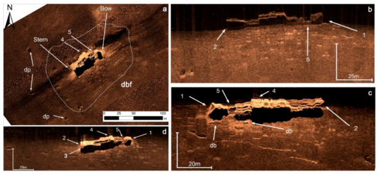
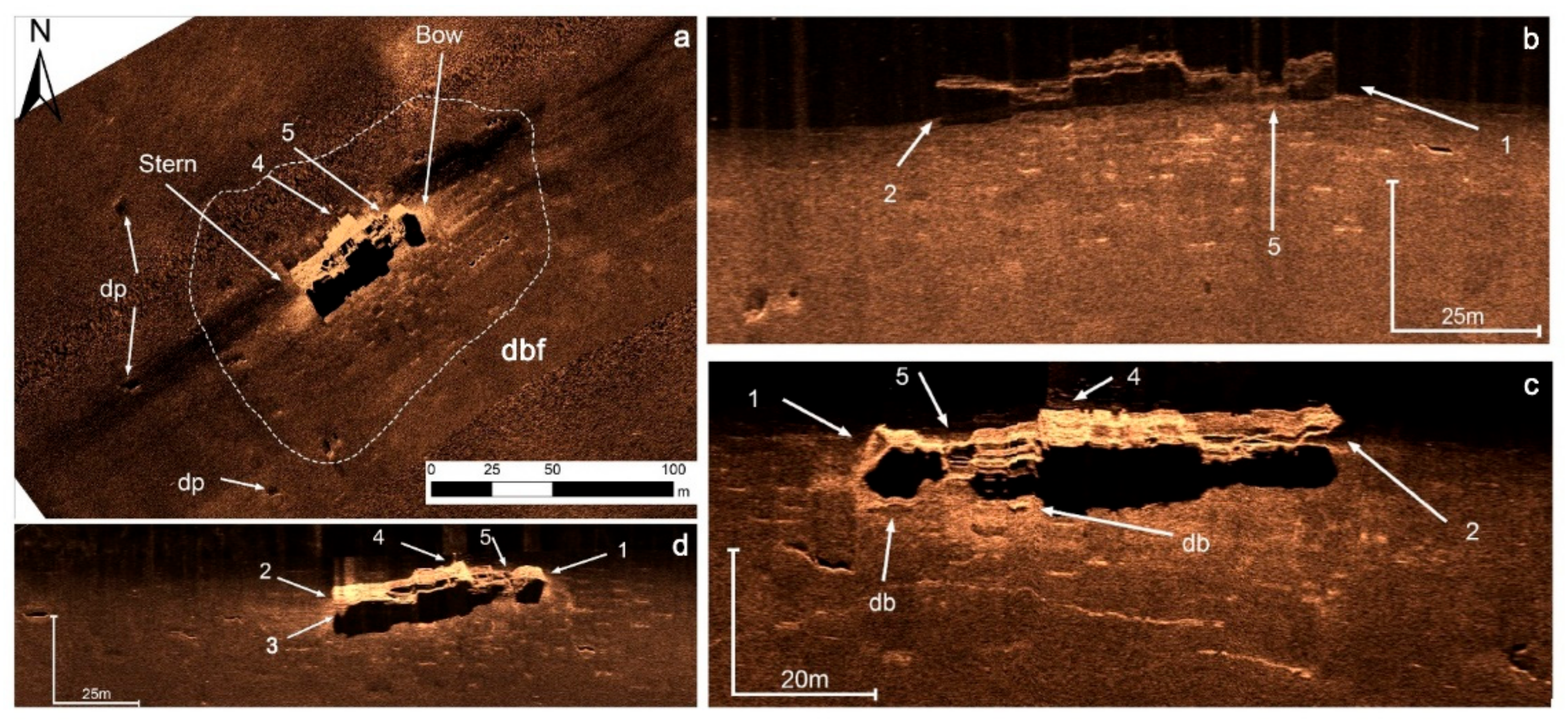
Figure 8.
(a) Regional 100 kHz sonograph showing the “pump house” wreck and its environment (dbf: debris field, db: wreck debris, dp: seabed depressions). (b–d) 500 kHz sonographs showing the main structural components of the “pump house” wreck (1: vertical bow or “plumb”, very common during the past half of the 19th century and the first decades of the 20th in merchant ships; 2: stern, 3: propellers; 4: bridge and 5: heavy damage on the bow).
5.2.2. “Pump House” Wreck and “Old Iron” Wreck
The marine remote sensing survey also revealed the presence of two steel wrecks: the “pump house” wreck and “old iron” wreck, initially detected by [15] and identified by [30].
The “pump house” wreck site is located 500 m west of the “many target” area, lies in an average water depth of 54 m and was identified as “SS Christoforos” by [30]. The length of the wreck is 60 m and its width is 17 m based on MBES measurements. The “SS Christoforos” was a cargo ship built in 1889 at Lübeck shipyards (Germany) as Kollund and then was renamed to “Alide”. She sunk on the 1st of February 1921 in heavy weather.
The seafloor sediments in the wreck site are characterized by a uniform low backscatter pattern, indicating that the wreck settled on a substrate of uniform, planar homogenous fine-grained sediments (Figure 8). The wreck lies on the seafloor and has a total length of 55 m from bow to stern (Figure 8). Sonographs taken at 400 kHz show the main structural components of the wreck, including the “plumb” or vertical bow, the bridge, the stern and the heavy damage at the bow (Figure 8). A debris field has been also recorded around the wreck containing many items spilled from the ship as it sank or by post-sinking man-made activities (mainly trawling). Tens of meters away from the wreck, the side-scan sonar survey also clearly imaged several small crater-like features (Figure 8). These features were interpreted as bomb craters by [15]. Although the visibility at the site of the “pump house” wreck was poor, ranging from less than 2 m above the seafloor to 3–4 m in the water column over the shipwreck, the R.O.V. survey inspected the main hull and the superstructure of the wreck. The bridge and the funnel of the vessel are almost intact and the aft and fore holds are empty and covered by mud. The wreck has been threatened by fishing activities, as indicated by the nets that are tangled around the bridge.
The side-scan sonar survey also successfully detected the “old iron” wreck. The wreck is located 3.4 km northeast of the “small target” area, very close to the site initially reported by [15]. In a recent survey [30], the authors suggested that the “old iron” wreck corresponds to the tugboat “Tanag33” based on remote sensing data, the visual inspection of the wreck and the available shipwreck database for the Patras Gulf. “Tanag33” attempted to tow sailing ship No123 of the Min Caique type but entered into a minefield due to mistaken navigation and finally sunk on 16 July of 1945. The wreck lies in an average water depth of 41 m and is oriented in a northeast–southwest direction. The length of the wreck as measured from the MBES bathymetry is 31 m and its width is 11 m. The resulting high-resolution sonographs showed that the hull of the wreck is not in one piece (Figure 9a–d). The bow has been partially separated from the hull of the wreck and is lying at about a 40–45° angle to the main hull (Figure 9a–d). The sonograph clearly shows the bow and the superstructures of the wreck (Figure 9d). A wreck debris field surrounds the wreckage site (Figure 9a,b,d). The most striking finding is the existence of numerous small-sized crater-like features around the “old iron” shipwreck at an average distance of about 50 m significantly higher than that reported by [30]. The same authors interpreted the small crater-like features as pockmarks (Figure 9b–d). The pockmarks form a well-developed pockmark field around the shipwreck (Figure 9a).
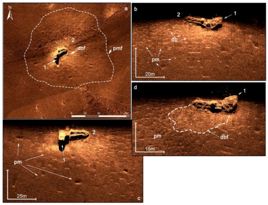
Figure 9.
(a) Regional 100 kHz sonograph showing the “old iron” wreck and its environment, (b–d) 500 kHz sonographs showing the main structural components of the “old iron” wreck (1: bow, 2: stern) (dbf: debris field, db: wreck debris, pm: pockmarks, pmf: pockmark field).
5.2.3. Shipwreck Site Formation Processes
The acquired sub-bottom profiling, bathymetric and side-scan sonar data from the two wreckage sites revealed two noticeable seafloor morphological features: (i) seafloor depressions and (ii) a field of small-sized craters, both surrounding the core of the wreckages. Therefore, these features can be considered to have been initiated by the introduction of the shipwrecks to the seafloor.
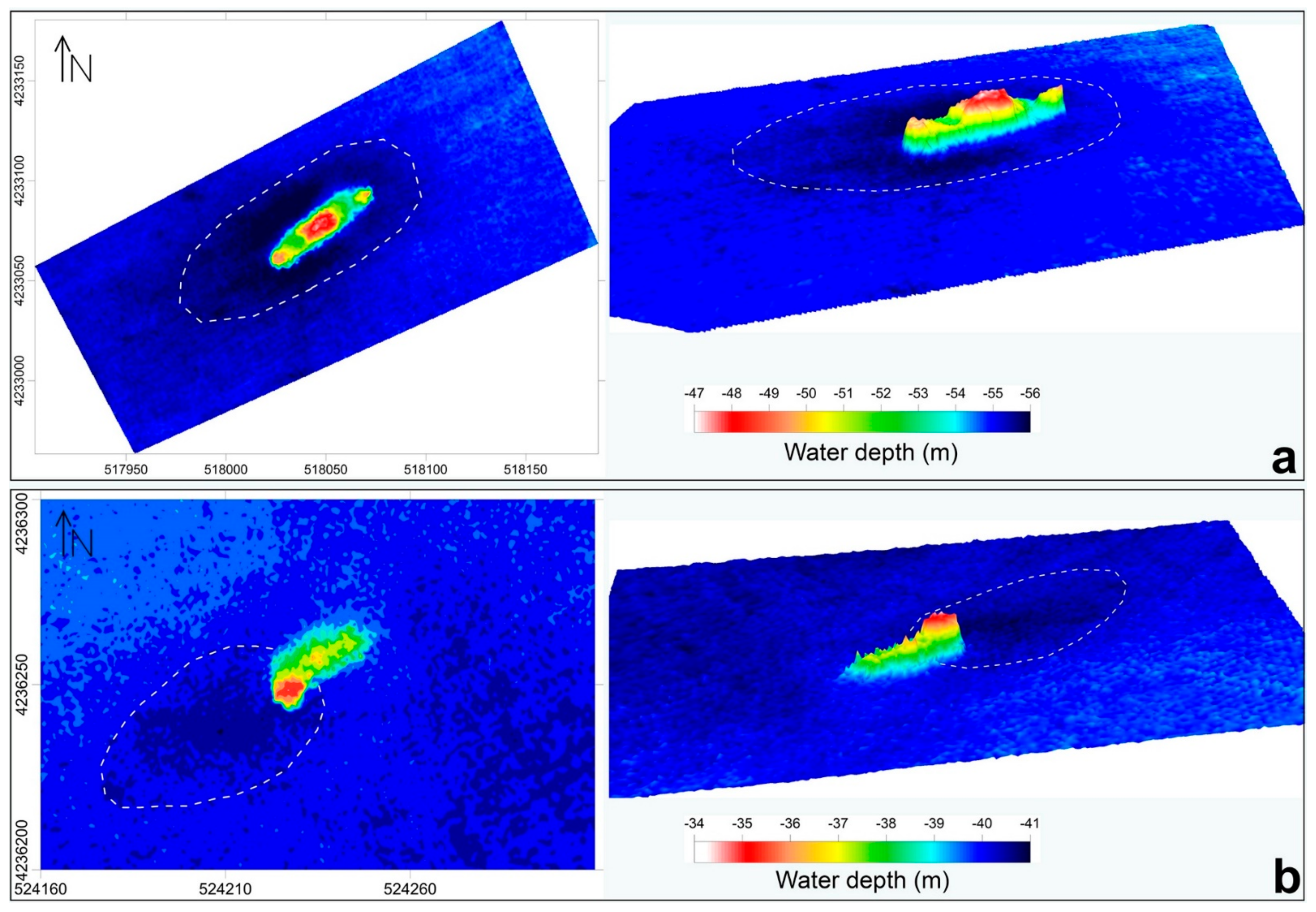
Bathymetric data together with sub-bottom profiling data clearly show seafloor depressions around the “pump house” wreck and the bow of the “old iron” wreck. The seafloor depression around the “pump house” wreck is almost elliptical-shaped, about 140 m long and 50 m wide and roughly 1 m deeper than the surrounding seabed (Figure 10a). The strong asymmetry in the depression around the shipwreck has been well documented. The stern-end of the depression is located 45 m from the stern, while the bow-end is about 15 m away from the bow of the shipwreck (Figure 10a). A teardrop-shaped depression has been also observed around the bow area of the “old iron” wreck (Figure 10b). The depression has a length of 40 m and a width of about 20 m and originates around the bow of the wreck extending southwest, parallel to the shipwreck axis (Figure 10b).
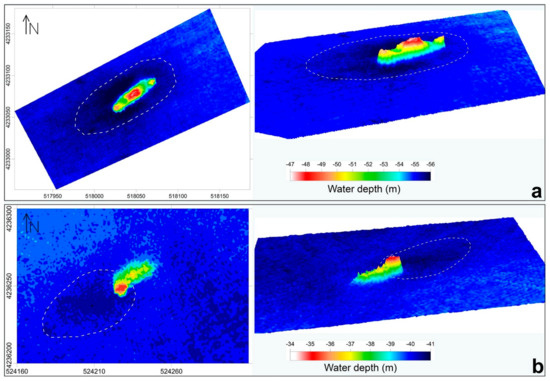
Figure 10.
Multibeam 2D and 3D bathymetric maps showing seafloor depressions around (a) the “pump house” wreck and (b) the bow of the “old iron” wreck.
Seafloor depressions as a result of scouring have been frequently observed around shipwrecks ([31] and references within). Scouring at wreck sites is controlled by a variety of factors, among which the most important is the hydrodynamic regime (currents, waves or combined waves and currents) [31]. Since the survey area is dominated by weak currents, the seafloor depressions around the shipwrecks cannot be considered as scour depressions.
The second noticeable seafloor formation detected mainly around the “old iron” wreck site and to a lesser extent close to the “pump house” wreck site consists of small-sized crater-like features (Figure 8 and Figure 9). These features are distributed in halos around the shipwreck sites. This distribution around the wrecks, with their mean location within a few tens of meters from each wreck, further suggests that the wrecks provide a nucleus for halo formation. In the “old iron” wreck site, the almost circular field consists of many craters and extends over an area of 13,000 m2 (Figure 9). The spacing of the individual craters ranges between 2.5 and 11 m, and they are widespread around the wreck in a radius of 70 m (Figure 9). The craters are mostly circular or oval in plan view, ranging from 2 to 3 m in diameter and up to 0.5 m in depth (Figure 9). The wreck is not located at the center of this field but at the southwestern end. The possibility of a ship sinking by chance on the seabed inside a field of craters seems extremely small. Moreover, few craters have been also observed in the vicinity of the “pump house” wreck, with a considerably larger size (−5 m) compared to those of the “old iron” wreck (Figure 8).
A reliable explanation for the existence of the craters is that they could have been formed by fluid flows escaping from the seafloor due to the loading of the wreck on the soft sediments of the seafloor. In that case, the crater-like features could be considered to be small-sized pockmarks. This explanation is also suggested by [30]. The crater-like nature of pockmarks suggests an erosional power of interstitial water venting commonly related to an overpressured, buried, unconsolidated sediment body and/or gas seepage related to an overpressured reservoir of biogenic/thermogenic gases [32].
There are few well-documented examples showing a possible causative relationship between pockmarks and shipwrecks which can be attributed either to the buoyancy loss of the ship due to gas emission from an active pockmark or to pockmark formation due to shipwreck loading on the soft seabed. In a marine geophysical survey [32], the authors mentioned the discovery of an almost intact shipwreck inside a large and shallow pockmark (Witch’s Hole) in the North Sea. In the same survey [32], the authors suggested that the location of the shipwreck at the center of the pockmark could be attributed to (i) the buoyancy loss of the ship due to vigorous gas release from the pre-existing pockmark and the consequent sinkage of the vessel inside the pockmark and (ii) the formation of the pockmark by the loading of the landing ship on the soft seafloor and the consequent escape of fluid flows. During a marine remote sensing survey [33], two other pockmarks also reported, similar in appearance to the Witch’s Hole pockmark, both with wreck-like targets lying in the very middle of the pockmarks. According to the author, this new evidence suggests that, rather than the ships being sunk by gas escapes, which seems extremely improbable, the impact of the ship hitting the seabed may have triggered the gas escaping and hence the formation of the pockmarks.
In a study of shipwrecks formation processes [34], the authors documented pockmark-like features around a shipwreck in N.E. Ireland. Their origin remains unknown, and the authors suggested that those features could be (i) traces of salvage operations conducted at the site in the past or (ii) pockmarks as a result of gas emission from the interstitials due to the excessive pressure on the sediments by the load of the shipwreck.
Moreover, researchers studying the Skagerrak seeps (North Sea) [35] reported that the seep area was located very close to a wreck. Furthermore, in a study of bioturbation around shipwrecks [36], the author detected a circular depression of 10 m in diameter around five wreck sites located at the Great Barrier Reef mid-shelf, and he interpreted them as formations of biological activity.
The size of the pockmarks around the “old iron” and “pump house” wrecks does not appear to be representative of vigorous gas discharge. Furthermore, the identification of the two steel wrecks excludes the loss of buoyancy as the cause of the ship’s sinking. The steel wreck load on the soft seabed is large enough to cause the deformation of the porous medium and pore water flow. When the wreck landed on the seabed, the load was applied to the seabed surface, excess pore water pressure was generated and pore water flowed out. The focused seepage from the porous medium could become a major factor for pockmark formation due to the erosional power of fluid venting. The fluid seepage could be enhanced by the existence of an overpressured, buried reservoir of biogenic and/or thermogenic gas.
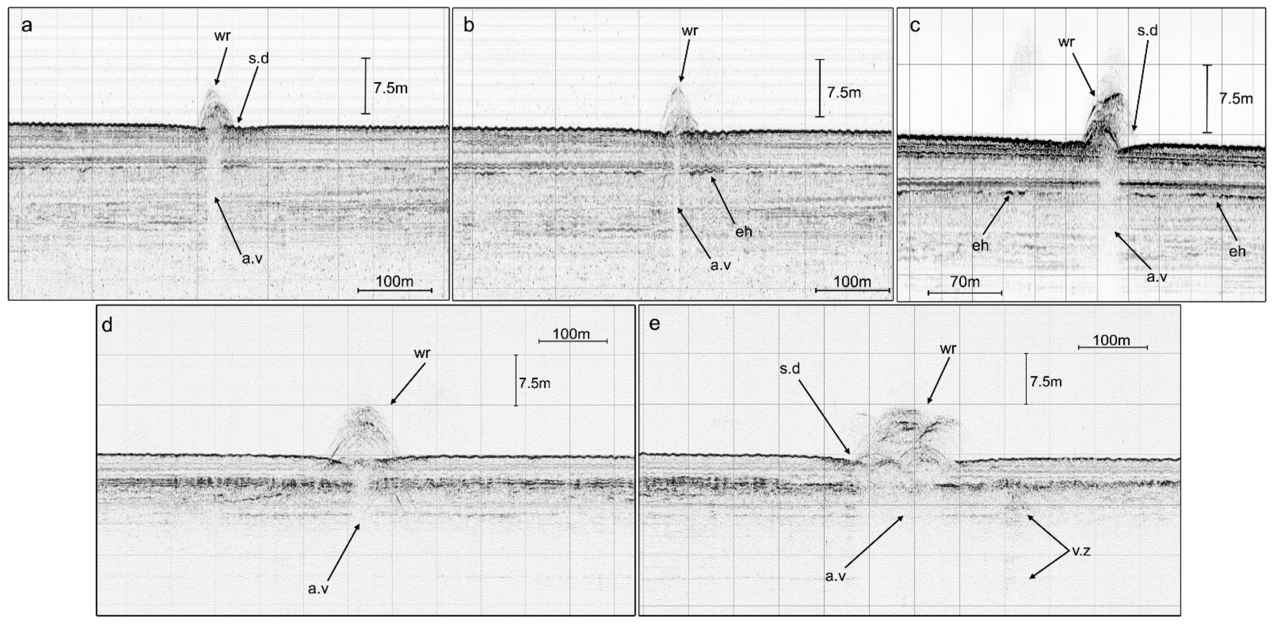
Chirp and 3.5 kHz seismic profiles were acquired for both wreck sites. Elevated multiple hyperbolic echoes indicate the existence of the wrecks. The vertex elevation of the hyperbolic echoes above the seafloor indicates the height of the wrecks at this section, suggesting a height of about 10 m for the “old iron” wreck and about 6 m for the “pump house” wreck (Figure 11). The prolonged hyperbolic echoes were formed by out-of-plane sound wave reflections off the wreck, which is characterized as an object of very high acoustic impedance. The well-developed acoustic void area seen below the hyperbolic echoes on the seismic profiles was produced due to the reflection of the sound waves by the very dense and solid body of the wrecks (Figure 11). This results in no acoustic return below the wreck and thus to the acoustic masking of the sub-bottom stratigraphy of the seafloor.
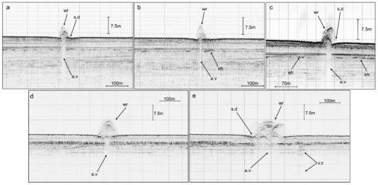
Figure 11.
(a,b) Profile at 3.5 kHz and (c) chirp profile across the “old iron” wreck and (d,e) chirp profiles of “pump house” wreck showing the multiple hyperbolic echoes due to the existence of the wrecks (wr) and the seabed depressions (s.d) around them (a.v: acoustic void area, eh: enhanced reflectors, v.z: vertical zone of acoustic anomalies).
The seismic data show that the underlying sediment stratigraphy is quite different for the two steel shipwrecks. The “pump house” wreck is lying on the top of the surface sequence (I), previously described as the upper sequence, consisting of parallel to subparallel reflectors with more weak reflectors and almost semi-transparent character at its base (Figure 11a–c). This surface sequence overlies sequence (II) with high amplitude reflectors. The “old iron” wreck is lying on the surface sequence (I), in that case overlying the chaotic sediment deposit (Figure 11d,e).
The seismic profiles do not reveal any clear acoustic anomaly indicative of gas-charged sediments. The only weak indication is the existence of enhanced reflectors below the wreck sites (Figure 11b,c). Moreover, vertical pore water and/or gas expulsions were detected in the vicinity of both shipwrecks. In one case, about 100 m southwest of the “pump house” wreck, a vertical zone of seismic anomalies was detected (Figure 11e). This feature possibly indicates vertical pore water and/or gas migration. No other amplitude anomalies (acoustic turbid zones, gas pockets, gas plumes) were observed on the profiles in the vicinity of the wreck sites. However, the absence of amplitude anomalies does not necessarily mean the absence of gas in the sediment interstices. Taking into consideration the fact that the Holocene/Pleistocene boundary in the Patras Gulf is a gas accumulation horizon [27,28], the minor contribution of gas seepage in the formation of the crater-like features cannot be excluded. Therefore, the craters detected around the wreckage sites can be interpreted as pockmarks formed by the erosional power of fluid venting.
Taking into consideration the above interpretation of the crater-like features, the seafloor depressions observed around the shipwrecks could also be interpreted as morphological features caused by the loading of the wrecks and consequently the compaction of the sediments.
5.2.4. Trawling Marks
The third acoustic backscatter pattern (ABP III) in the side-scan sonar data does not correlate with any changes in the acoustic signal in the seismic profiles, suggesting a superficial geomorphological character (Figure 3 and Figure 4). The linear features of ABP III are interpreted as marks produced by bottom-fishing gear. It is well known that the northern part of Patras Gulf has been an active commercial fishing ground for bottom-fishing gear, particularly trawls [26]. Both survey areas (“many target” and “small target”) constitute parts of this extensive fishing ground. Trawls normally interact with the seafloor through two trawl doors leaving two parallel tracks, scouring and flattening the seabed with ropes and weights and redistributing or removing sediment and other man-made objects [37]. In most cases, the side-scan sonar tracklines are almost parallel to trawling axis, and the trawl marks are relatively clear and countable on the images. In the cross-track side-scan sonar images, the trawl marks are less evident but are still well defined and countable. The trawl marks observed on the side-scan sonar records are very dense and thus are very rarely noted as being paired.
The main axes of trawling are 345° and 313° in the “many target” and “small target” areas, respectively, following the depth contours as well as the prevailing wind direction. Although the mean density of trawl marks is significant pover the entire studied area (491 trawl marks/km2), their presence is more enhanced in the “small target” area (610 trawl marks/km2 with a total length of 166 km) compared to the “many target” area (336 trawl marks/km2 with a total length of 78 km). The higher accumulation of trawl marks in the “small target” area suggests higher fishing activity, resulting in a flattening or weakening of the mounds at this site and consequently to the reduction of their reflectivity. The lower reflectivity of the mounds observed in the “small target” area compared to that of the “many target” area is fully explained by the more intense fishing activity (Figure 3 and Figure 4).
In [15], the authors did not report any trawl marks, although parallel to sub-parallel scours can be detected on the sonograph where the “pump house” wreck is presented ([15]: 128, Figure 8). However, at the time when the survey was carried out [15], the fishing trawlers were wooden vessels with much lighter gear, and thus the trawl marks on the seafloor—and consequently their acoustic signatures—were weakened.
Unfortunately, trawl fishery is very common at sites of archaeological interest. Wrecks or remnants of wrecks usually develop into artificial reefs of enhanced biological activity; this attracts that kind of fishery, which often damages the site.
5.2.5. Future Work
Although the present remote sensing survey did not show any indication of wreck remnants of the Battle of Lepanto within the two surveyed areas, the wider area constitutes a very promising environment for applying innovative methodological approaches and systems [38,39,40]. The MBES with multispectral backscatter capabilities provides backscatter at multiple frequencies from a single pass over the survey seabed and improves our understanding of seafloor morphology, particularly in areas with scattered mounds [40]. The parametric sub-bottom profiler transmits two primary simultaneous high-frequency signals at high sound pressure and provides ultra-high-resolution seismic profiles. Parametric SBP is an ideal tool for the detection of embedded objects of archaeological importance [41] and could provide valuable information for potential buried targets in the “small target” and “many target” areas. Moreover, the core sampling of undisturbed sediments, collected within both areas, combined with dating techniques (e.g., radiocarbon dating) would offer an estimation of the sedimentation rate of the wider area and consequently the burial depth of the remnants of the Battle of Lepanto [42].
6. Conclusions
A series of marine remote sensing and ground-truth surveys were carried out at the NW Gulf of Patras, in the same area that was surveyed in 1971 by Throckmorton, Edgerton and Yalouris to locate the site at which the Battle of Lepanto took place on 7 October 1571. The marine remote sensing survey of those pioneers resulted in the detection of promising “targets” located in two areas (“many target” and “small target”) and two steel shipwrecks. A ground-truthing survey for the identification of “targets” was proposed by those researchers, but this final step never took place. Our repeat surveys detected mound clusters and individual mounds referred to as “many and small targets” areas by [15]. These two areas are further distinguished based on the spatial density of the clusters and their acoustic backscatter characteristics. Based on high-resolution sub-bottom profiling data, the mounds can be interpreted as the surface expression of mud and fluid expulsion from the underlying deformed soft sediments. The ground-truthing survey demonstrated that the tops of mounds represent biogenic mounds quite similar to the coralline algae reefs reported in the Aegean Sea. Small sponges, polychaetes and soft-tissue corals cover the top of the mounds. The ROV survey did not show any indication of wreck remnants of the Battle of Lepanto within the two survey areas. The site formation processes of the two shipwrecks—the “pump house” (SS Christoforos) and “old iron” (Tanag 33) shipwrecks—have also been studied in detail. Two noticeable seafloor morphological features have been detected around the wreck sites: fields of small-sized craters and seafloor depressions. Based on the side-scan sonar and profiling data, those craters can be interpreted as small-sized pockmarks formed by the erosional power of fluid venting. The load of the steel wrecks on the soft seabed is large enough to cause the deformation of the porous medium and pore water flow. The seafloor depressions observed around the shipwrecks could be also interpreted as morphological features caused by the loading of the wrecks and consequently the compaction of the sediments. Both mound areas have been heavily affected by bottom fishing activity, as indicated by the dense trawl marks recorded on the sonographs.
Author Contributions
Conceptualization and writing, G.P.; writing, M.G.; data acquisition and analysis, D.C., E.F.; data acquisition, M.I., N.G., X.D.; data analysis and editing, N.G., X.D.; editing, G.F. All authors have read and agreed to the published version of the manuscript.
Funding
This study was funded by the Laboratory of Marine Geology and Physical Oceanography (Oceanus-lab, https://oceanus-lab.upatras.gr/, accessed date 1 July 2021).
Acknowledgments
G. Karelas, M. Patsourakis, M. Prevenios and S. Sergiou are gratefully thanked for their assistance in acquiring the data. The authors would also like to thank the captain and the crew of “IRENE” NP 464 and “Milady Mylord III”, ΝP 488 for their help during the research cruises.
Conflicts of Interest
The authors declare no conflict of interest.
References
- Frey, D. Sub-bottom survey of Porto Longo harbour, Peleponnesus, Greece. Int. J. Naut. Archaeol. 1972, 1, 170–175. [Google Scholar] [CrossRef]
- Scoufopoulos, N.C.; Mckernan, J.G. Underwater survey of ancient Gythion, 1972. Int. J. Naut. Archaeol. 1975, 4, 103–116. [Google Scholar] [CrossRef]
- Papatheodorou, G.; Stefatos, A.; Christodoulou, D.; Ferentinos, G. Remote sensing in submarine archaeology and marine cultural resources management: An ancient shipwreck outside Zakynthos port, Greece. In Proceedings of the 7th International Conference on Environmental Science and Technology, Ermoupolis, Syros Island, Greece, 3–6 September 2001; Volume C, pp. 377–385. [Google Scholar]
- Papatheodorou, G.; Geraga, M.; Ferentinos, G. The Navarino Naval Battle site, Greece—An integrated remote-sensing survey and a rational management approach. Int. J. Naut. Archaeol. 2005, 34, 95–109. [Google Scholar] [CrossRef]
- Papatheodorou, G. Ghostly images of HMHS britannic. Hydro Int. 2008, 12, 15–18. [Google Scholar]
- Delaporta, K.; Jasinski, M.E.; Søreide, F. The Greek-Norwegian Deep-Water Archaeological Survey. Int. J. Naut. Archaeol. 2006, 35, 79–87. [Google Scholar] [CrossRef]
- Sakellariou, D.; Georgiou, P.; Mallios, A.; Kapsimalis, V.; Kourkoumelis, D.; Micha, P.; Theodoulou, T.; Dellaporta, K. Searching for ancient shipwrecks in the aegean sea: The discovery of chios and kythnos hellenistic wrecks with the use of marine Geological-geophysical methods. Int. J. Naut. Archaeol. 2007, 36, 365–381. [Google Scholar] [CrossRef]
- Geraga, M.; Papatheodorou, G.; Ferentinos, G.; Fakiris, E.; Christodoulou, D.; Georgiou, N.; Dimas, X.; Iatrou, M.; Kordella, S.; Sotiropoulos, G.; et al. The study of an ancient shipwreck using marine remote sensing techniques, in Kefalonia Island (Ionian Sea), Greece. Archaeol. Marit. Mediterr. 2015, 12, 183–200. [Google Scholar]
- Ferentinos, G.; Fakiris, E.; Christodoulou, D.; Geraga, M.; Dimas, X.; Georgiou, N.; Kordella, S.; Papatheodorou, G.; Prevenios, M.; Sotiropoulos, M. Optimal sidescan sonar and sub-bottom profiler surveying of ancient wrecks: The ‘Fiskardo’ wreck, Kefallinia Island, Ionian Sea. J. Archaeol. Sci. 2020, 113, 105032. [Google Scholar] [CrossRef]
- Ferentinos, G.; Gkioni, M.; Geraga, M.; Papatheodorou, G. Early seafaring activity in the southern Ionian Islands, Mediterranean Sea. J. Archaeol. Sci. 2012, 39, 2167–2176. [Google Scholar] [CrossRef]
- Ballard, R.D.; McCann, A.M.; Yoerger, D.; Whitcomb, L.; Mindell, D.; Oleson, J.; Singh, H.; Foley, B.; Adams, J.; Piechota, D.; et al. The discovery of ancient history in the deep sea using advanced deep submergence technology. Deep Sea Res. Part I Oceanogr. Res. Pap. 2000, 47, 1591–1620. [Google Scholar] [CrossRef]
- Quinn, R.; Bull, J.M.; Dix, J.K.; Adams, J.R. The Mary Rose site–geophysical evidence for palaeo-scour marks. Int. J. Naut. Archaeol. 1997, 26, 3–16. [Google Scholar] [CrossRef] [Green Version]
- Quinn, R.; Adams, J.; Dix, J.; Bull, J. The (1758) site—An integrated geophysical assessment. Int. J. Naut. Archaeol. 1998, 27, 126–138. [Google Scholar] [CrossRef]
- Quinn, R.; Breen, C.; Forsythe, W.; Barton, K.; Rooney, S.; O’Hara, D. Integrated Geophysical Surveys of The French Frigate La Surveillante (1797), Bantry Bay, Co. Cork, Ireland. J. Archaeol. Sci. 2002, 29, 413–422. [Google Scholar] [CrossRef]
- Throckmorton, P.; Edgerton, H.E.; Yalouris, E. The Battle of Lepanto search and survey mission (Greece), 1971–1972. Int. J. Naut. Archaeol. 1973, 2, 121–130. [Google Scholar] [CrossRef]
- Setton, K. Venice, Austria, and the Turks in the Seventeenth Century; American Philosophical Society: Philadelphia, PA, USA, 1991. [Google Scholar]
- Konstam, A.; Bryan, T. Lepanto, 1571: The Greatest Naval Battle of the Renaissance; Osprey Publishing: Oxford, UK, 2005; ISBN 1841764094. [Google Scholar]
- Hess, A.C. The Battle of Lepanto and its place in Mediterranean History. Past Present 1972, 57, 53–73. [Google Scholar] [CrossRef]
- Vött, A. Silting up Oiniadai’s harbours (Acheloos River delta, NW Greece). Geoarchaeological implications of late Holocene landscape changes. Géomorphol. Reli. Process. Environ. 2007, 13. [Google Scholar] [CrossRef] [Green Version]
- Vött, A.; Brückner, H.; Schriever, A.; Handl, M.; Besonen, M.; Borg, K. Van Der Holocene coastal evolution around the ancient seaport of Oiniadai, Acheloos alluvial plain, NW Greece. Geogr. Der Meere Und Küsten 2004, 1, 43–53. [Google Scholar]
- Poulos, S.E. Sediment yield of Greek rivers. In Proceedings of the 5th Panhellenic Symposium of Oceanography and Fisheries, Kavala, Greece, 15–18 April 1997; pp. 481–482. [Google Scholar]
- Piper, D.J.W.; Panagos, A.G. Surficial Sediments of the Gulf of Patras. Thalassographica 1979, 3, 5–20. [Google Scholar]
- Chronis, G.; Piper, D.J.W.; Anagnostou, C. Late Quaternary evolution of the Gulf of Patras, Greece: Tectonism, deltaic sedimentation and sea-level change. Mar. Geol. 1991, 97, 191–209. [Google Scholar] [CrossRef]
- Ferentinos, G.; Brooks, M.; Doutsos, T. Quaternary tectonics in the Gulf of Patras, western Greece. J. Struct. Geol. 1985, 7, 713–717. [Google Scholar] [CrossRef]
- Fourniotis, N.T.; Horsch, G.M. Three-dimensional numerical simulation of wind-induced barotropic circulation in the Gulf of Patras. Ocean Eng. 2010, 37, 355–364. [Google Scholar] [CrossRef]
- Tzanatos, E.; Somarakis, S.; Tserpes, G.; Koutsikopoulos, C. Identifying and classifying small-scale fisheries métiers in the Mediterranean: A case study in the Patraikos Gulf, Greece. Fish. Res. 2006, 81, 158–168. [Google Scholar] [CrossRef]
- Papatheodorou, G.; Hasiotis, T.; Ferentinos, G. Gas-charged sediments in the Aegean and Ionian Seas, Greece. Mar. Geol. 1993, 112, 171–184. [Google Scholar] [CrossRef]
- Hasiotis, T.; Papatheodorou, G.; Kastanos, N.; Ferentinos, G. A pockmark field in the Patras Gulf (Greece) and its activation during the 14/7/93 seismic event. Mar. Geol. 1996, 130, 333–344. [Google Scholar] [CrossRef]
- Georgiadis, M.; Papatheodorou, G.; Tzanatos, E.; Geraga, M.; Ramfos, A.; Koutsikopoulos, C.; Ferentinos, G. Coralligène formations in the eastern Mediterranean Sea: Morphology, distribution, mapping and relation to fisheries in the southern Aegean Sea (Greece) based on high-resolution acoustics. J. Exp. Mar. Biol. Ecol. 2009, 368, 44–58. [Google Scholar] [CrossRef]
- Geraga, M.; Christodoulou, D.; Eleftherakis, D.; Papatheodorou, G.; Fakiris, E.; Dimas, X.; Georgiou, N.; Kordella, S.; Prevenios, M.; Iatrou, M.; et al. Atlas of Shipwrecks in Inner Ionian Sea (Greece): A Remote Sensing Approach. Heritage 2020, 3, 1210–1236. [Google Scholar] [CrossRef]
- Quinn, R. The role of scour in shipwreck site formation processes and the preservation of wreck-associated scour signatures in the sedimentary record—Evidence from seabed and sub-surface data. J. Archaeol. Sci. 2006, 33, 1419–1432. [Google Scholar] [CrossRef]
- Judd, A.; Hovland, M. Seabed Fluid Flow. In The Impact on Geology, Biology and the Marine Environment; Cambridge University Press: Cambridge, UK, 2007. [Google Scholar]
- Judd, A. Pockmarks in the UK sector of the North Sea. Tech. Rep. Prod. Strateg. Environ. Assess. SEA2 2001, 71, 1–20. [Google Scholar]
- Majcher, J.; Quinn, R.; Plets, R.; Coughlan, M.; McGonigle, C.; Sacchetti, F.; Westley, K. Spatial and temporal variability in geomorphic change at tidally influenced shipwreck sites: The use of time-lapse multibeam data for the assessment of site formation processes. Geoarchaeology 2021, 36, 429–454. [Google Scholar] [CrossRef]
- Dando, P.R.; Bussmann, I.; Niven, S.J.; O’Hara, S.C.M.; Schmalijohann, R.; Taylor, L.J. A methane seep area in the Skagerrak, the habitat of the pogonophore Siboglinum poseidoni and the bivalve mollusc Thyasira sarsi. Mar. Ecol. Prog. Ser. 1994, 107, 157–168. [Google Scholar] [CrossRef]
- Stieglitz, T.C. Habitat engineering by decadal-scale bioturbation around shipwrecks on the Great Barrier Reef mid-shelf. Mar. Ecol. Prog. Ser. 2013, 477, 29–40. [Google Scholar] [CrossRef] [Green Version]
- Smith, C.J.; Banks, A.C.; Papadopoulou, K.-N. Improving the quantitative estimation of trawling impacts from sidescan-sonar and underwater-video imagery. ICES J. Mar. Sci. 2007, 64, 1692–1701. [Google Scholar] [CrossRef] [Green Version]
- Yang, F.; Xu, F.; Zhang, K.; Bu, X.; Hu, H.; Anokye, M. Characterisation of terrain variations of an underwater ancient town in Qiandao Lake. Remote Sens. 2020, 12, 268. [Google Scholar] [CrossRef] [Green Version]
- Missiaen, T.; Evangelinos, D.; Claerhout, C.; De Clercq, M.; Pieters, M.; Demerre, I. Archaeological prospection of the nearshore and intertidal area using ultra-high resolution marine acoustic techniques: Results from a test study on the Belgian coast at Ostend-Raversijde. Geoarchaeology 2018, 33, 386–400. [Google Scholar] [CrossRef]
- Pydyn, A.; Popek, M.; Kubacka, M.; Janowski, Ł. Exploration and reconstruction of a medieval harbour using hydroacoustics, 3-D shallow seismic and underwater photogrammetry: A case study from Puck, southern Baltic Sea. Archaeol. Prospect. 2021, 1–16. [Google Scholar] [CrossRef]
- Papatheodorou, G.; Geraga, M.; Georgiou, N.; Christodoulou, D.; Dimas, X.; Fakiris, E.; Ferentinos, G. The palaeogeography of the strait of Salamis: Marine geoarchaeological survey in the strait of Salamis and the Ampelakia Bay. In Salamis 480 B.C.; Hellenic Maritime Museum: Athens, Greece, 2020; pp. 392–411. ISBN 139786188218178. [Google Scholar]
- Geraga, M.; Papatheodorou, G.; Agouridis, C.; Kaberi, H.; Iatrou, M.; Christodoulou, D.; Fakiris, E.; Prevenios, M.; Kordella, S.; Ferentinos, G. Palaeoenvironmental implications of a marine geoarchaeological survey conducted in the SW Argosaronic gulf, Greece. J. Archaeol. Sci. Rep. 2017, 12, 805–818. [Google Scholar] [CrossRef] [Green Version]


Publisher’s Note: MDPI stays neutral with regard to jurisdictional claims in published maps and institutional affiliations. |
© 2021 by the authors. Licensee MDPI, Basel, Switzerland. This article is an open access article distributed under the terms and conditions of the Creative Commons Attribution (CC BY) license (https://creativecommons.org/licenses/by/4.0/).