
IONORING: Real-Time Monitoring of the Total Electron Content over Italy


Abstract
:1. Introduction
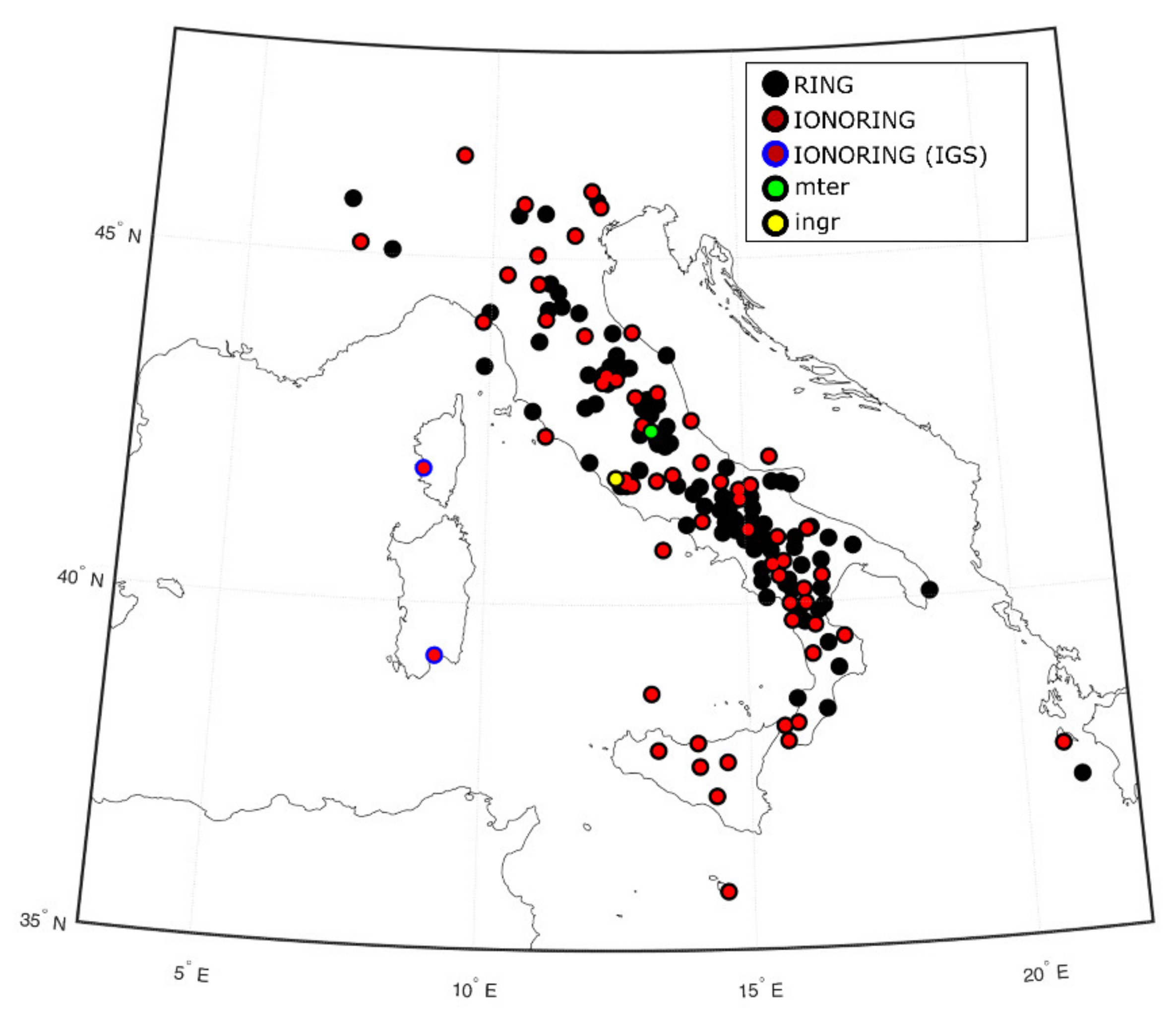
2. Data and Method
- Download of RINEX files for all the GNSS stations for the previous 3 days;
- Evaluation of for each satellite-receiver pair for the previous 3 days by applying Gg calibration technique;
- Calculation of the mean value over the previous 3 days for each satellite-receiver pair ();
- Creation of a lookup table containing m x n values, being m the total number of RING stations, n the total number of operating GPS satellites.
3. Results
4. Discussion
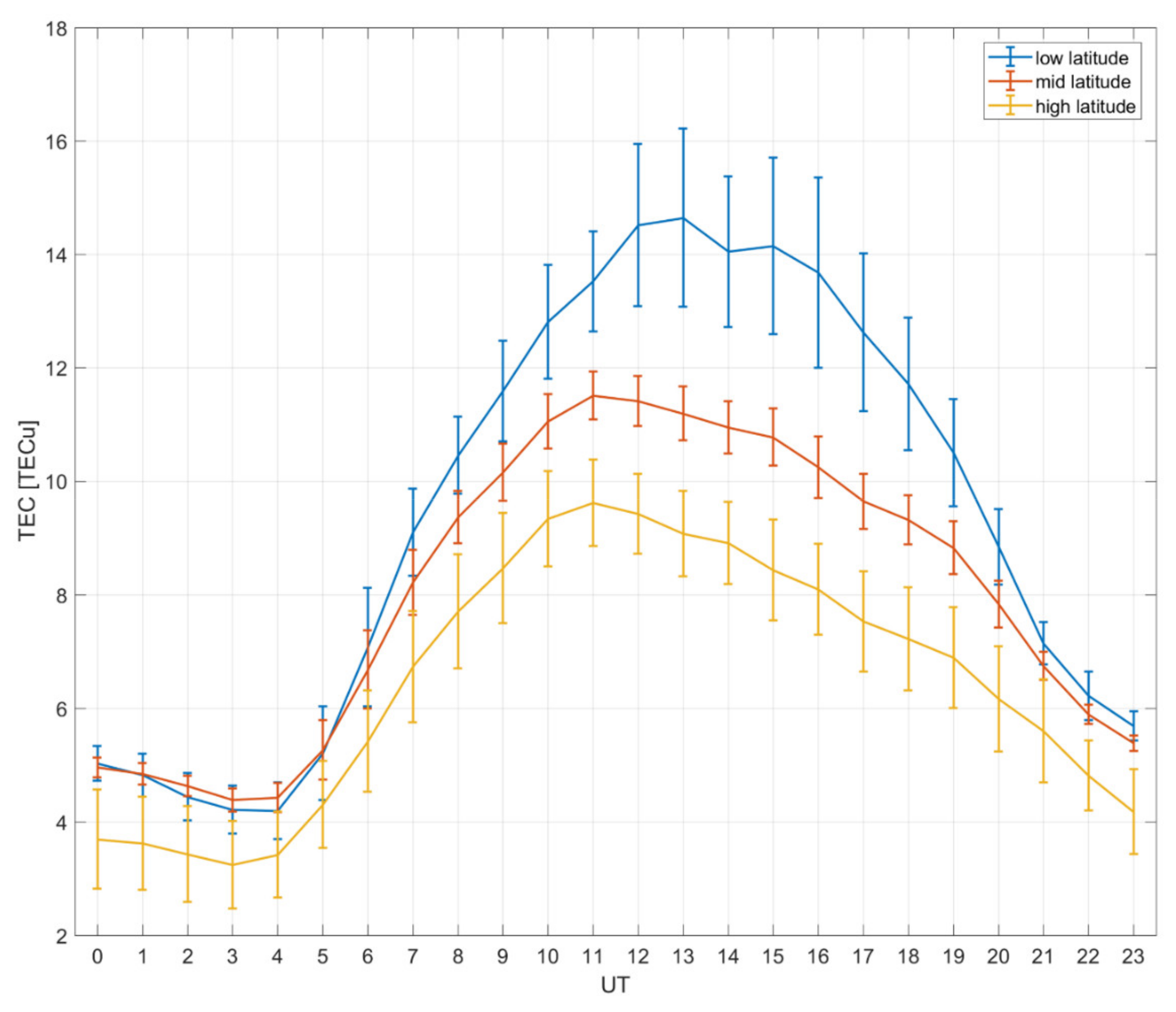
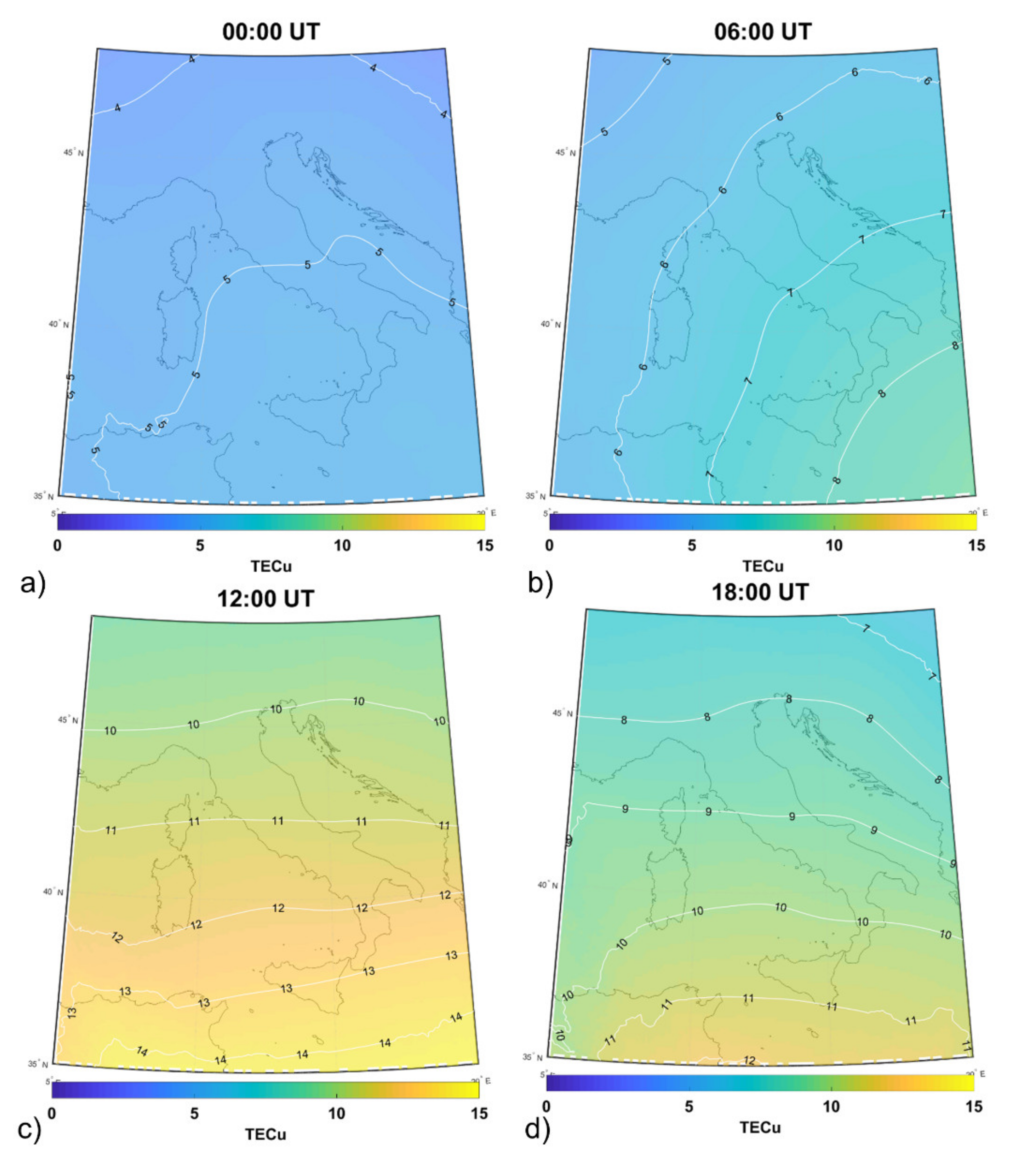
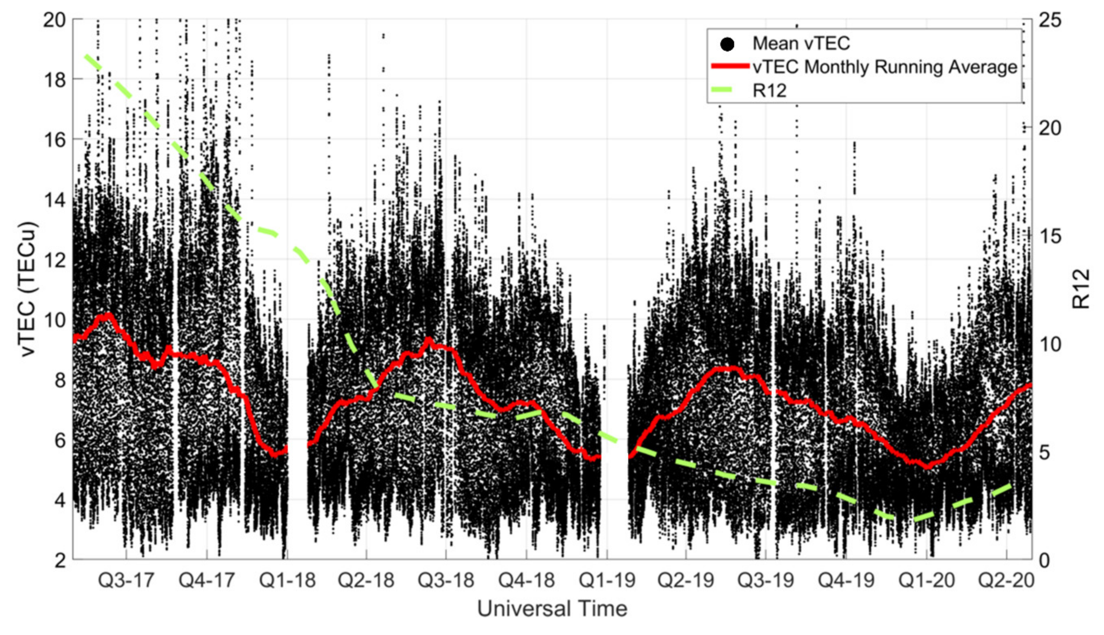
4.1. Seasonal, Daily and Latitudinal Variations
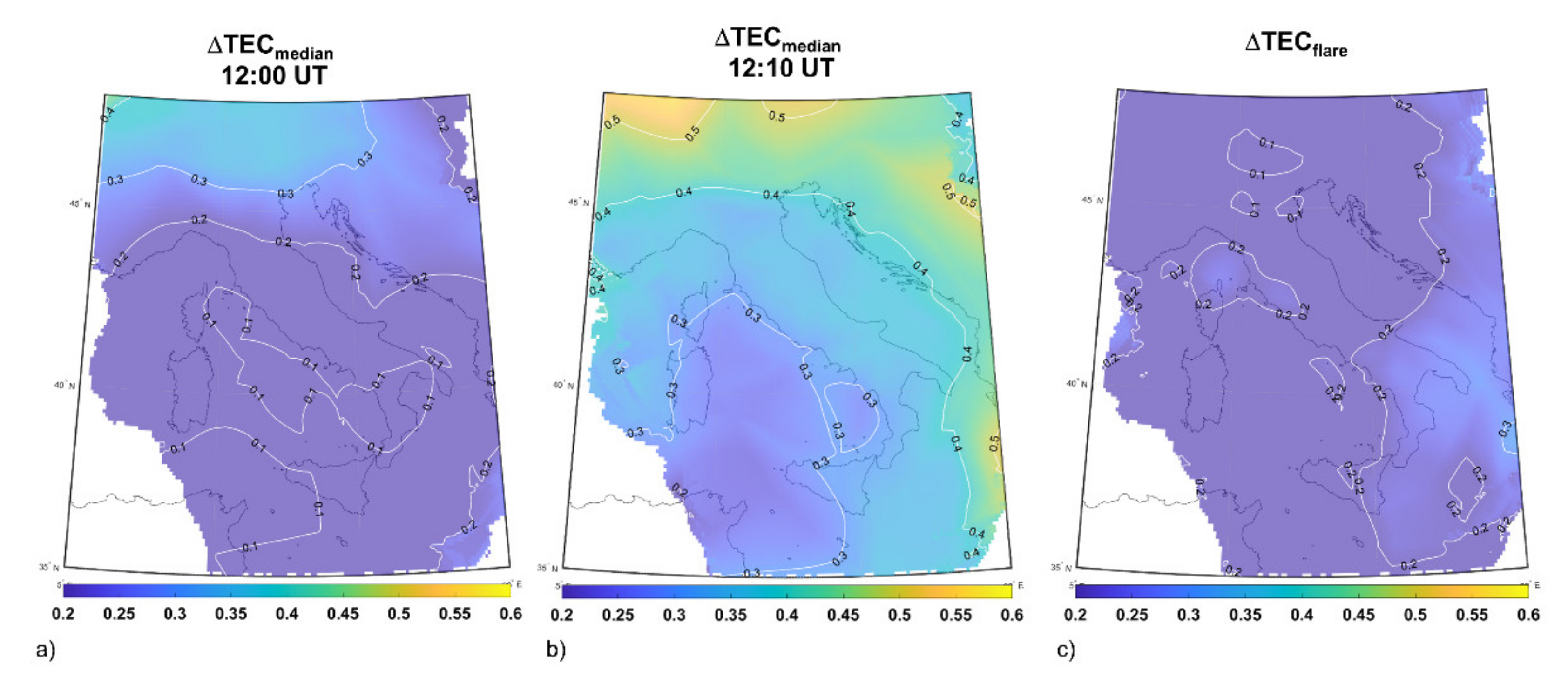
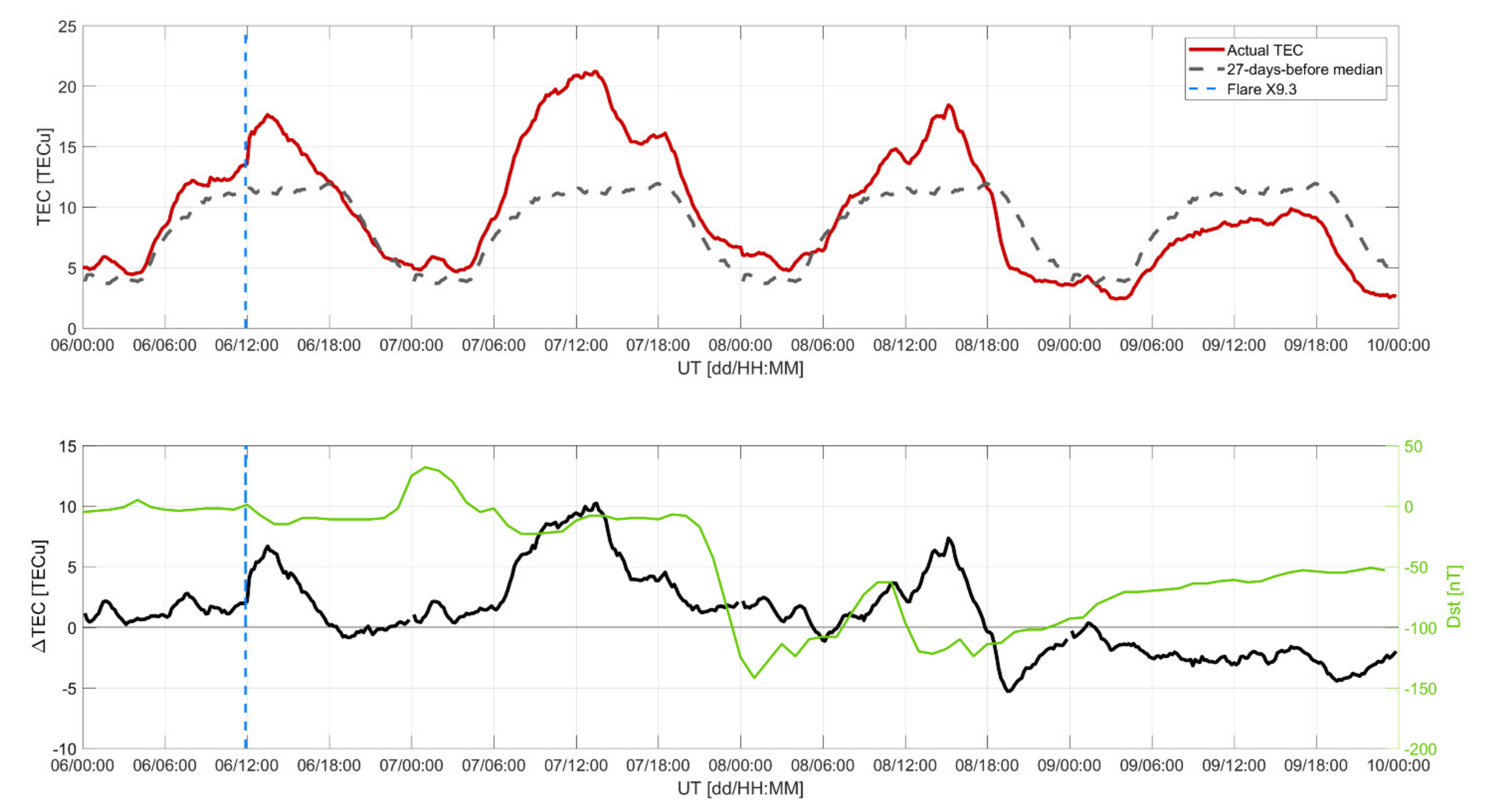
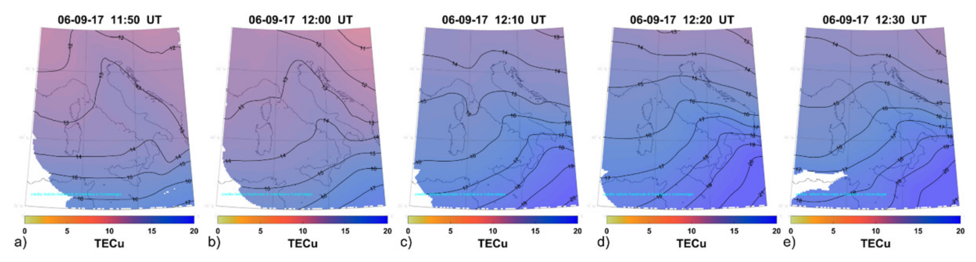
4.2. September 2017 Geomagnetic Storm
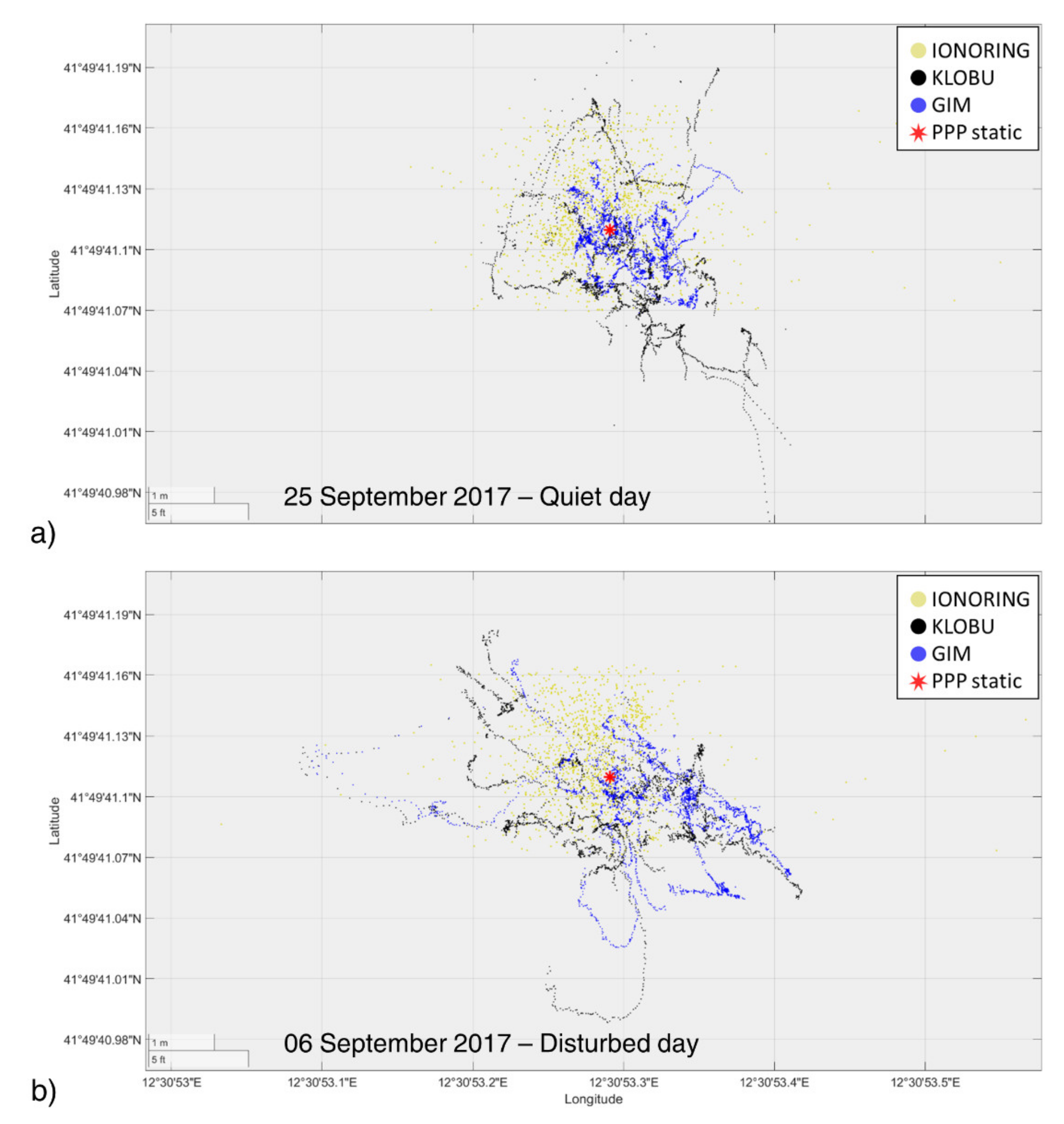
4.3. Application on Positioning
5. Conclusions
Author Contributions
Funding
Institutional Review Board Statement
Informed Consent Statement
Data Availability Statement
Acknowledgments
Conflicts of Interest
References
- Schrijver, C.J. Socio-Economic Hazards and Impacts of Space Weather: The Important Range between Mild and Extreme. Space Weather 2015, 13, 524–528. [Google Scholar] [CrossRef] [Green Version]
- De Franceschi, G.; Spogli, L.; Alfonsi, L.; Romano, V.; Cesaroni, C.; Hunstad, I. The ionospheric irregularities climatology over Svalbard from solar cycle 23. Sci. Rep. 2019, 9, 1–14. [Google Scholar] [CrossRef] [Green Version]
- Spogli, L.; Cesaroni, C.; Di Mauro, D.; Pezzopane, M.; Alfonsi, L.; Musicò, E.; Povero, G.; Pini, M.; Dovis, F.; Romero, R.; et al. Formation of ionospheric irregularities over Southeast Asia during the 2015 St. Patrick’s Day storm. J. Geophys. Res. Space Phys. 2016, 121, 12,211–12,233. [Google Scholar] [CrossRef]
- Spogli, L.; Sabbagh, D.; Regi, M.; Cesaroni, C.; Perrone, L.; Alfonsi, L.; Di Mauro, D.; Lepidi, S.; Campuzano, S.A.; Marchetti, D.; et al. Ionospheric Response Over Brazil to the August 2018 Geomagnetic Storm as Probed by CSES-01 and Swarm Satellites and by Local Ground-Based Observations. J. Geophys. Res. Space Phys. 2021, 126. [Google Scholar] [CrossRef]
- Mannucci, A.J.; Tsurutani, B.T.; Iijima, B.A.; Komjathy, A.; Saito, A.; Gonzalez, W.D.; Guarnieri, F.L.; Kozyra, J.U.; Skoug, R. Dayside global ionospheric response to the major interplanetary events of 29–30 October 2003 “Halloween Storms”. Geophys. Res. Lett. 2005, 32. [Google Scholar] [CrossRef] [Green Version]
- Yang, Z.; Mrak, S.; Morton, Y.J. Geomagnetic Storm Induced Mid-latitude Ionospheric Plasma Irregularities and Their Implications for GPS Positioning over North America: A Case Study. In Proceedings of the 2020 IEEE/ION Position, Location and Navigation Symposium (PLANS), Portland, OR, USA, 20–23 April 2020; pp. 234–238. [Google Scholar] [CrossRef]
- Ledvina, B.M.; Makela, J.; Kintner, P.M. First observations of intense GPS L1 amplitude scintillations at midlatitude. Geophys. Res. Lett. 2002, 29, 4-1–4-4. [Google Scholar] [CrossRef]
- Balan, N.; Liu, L.; Le, H. A brief review of equatorial ionization anomaly and ionospheric irregularities. Earth Planet. Phys. 2018, 2, 1–19. [Google Scholar] [CrossRef]
- Li, G.; Ning, B.; Otsuka, Y.; Abdu, M.A.; Abadi, P.; Liu, Z.; Spogli, L.; Wan, W. Challenges to Equatorial Plasma Bubble and Ionospheric Scintillation Short-Term Forecasting and Future Aspects in East and Southeast Asia. Surv. Geophys. 2020, 42, 201–238. [Google Scholar] [CrossRef]
- Shiokawa, K.; Otsuka, Y.; Ogawa, T.; Balan, N.; Igarashi, K.; Ridley, A.; Knipp, D.; Saito, A.; Yumoto, K. A large-scale traveling ionospheric disturbance during the magnetic storm of 15 September 1999. J. Geophys. Res. Space Phys. 2002, 107, SIA 5-1–SIA 5-11. [Google Scholar] [CrossRef] [Green Version]
- Zakharenkova, I.; Astafyeva, E.; Cherniak, I. GPS and GLONASS observations of large-scale traveling ionospheric disturbances during the 2015 St. Patrick’s Day storm. J. Geophys. Res. Space Phys. 2016, 121, 12,138–12,156. [Google Scholar] [CrossRef]
- Cesaroni, C.; Alfonsi, L.; Pezzopane, M.; Martinis, C.; Baumgardner, J.; Wroten, J.; Mendillo, M.; Musicò, E.; Lazzarin, M.; Umbriaco, G. The First Use of Coordinated Ionospheric Radio and Optical Observations Over Italy: Convergence of High-and Low-Latitude Storm-Induced Effects. J. Geophys. Res. Space Phys. 2017, 122, 11,794–11,806. [Google Scholar] [CrossRef]
- Park, J.; Sreeja, V.; Aquino, M.; Cesaroni, C.; Spogli, L.; Dodson, A.; De Franceschi, G. Performance of ionospheric maps in support of long baseline GNSS kinematic positioning at low latitudes. Radio Sci. 2016, 51, 429–442. [Google Scholar] [CrossRef] [Green Version]
- Klobuchar, J.A. Ionospheric Time-Delay Algorithm for Single-Frequency GPS Users. IEEE Trans. Aerosp. Electron. Syst. 1987, AES-23, 325–331. [Google Scholar] [CrossRef]
- Yuan, Y.; Wang, N.; Li, Z.; Huo, X. The BeiDou global broadcast ionospheric delay correction model (BDGIM) and its preliminary performance evaluation results. NAVIGATION 2019, 66, 55–69. [Google Scholar] [CrossRef] [Green Version]
- Yuan, Y.; Ou, J. Auto-covariance estimation of variable samples (ACEVS) and its application for monitoring random ionospheric disturbances using GPS. J. Geod. 2001, 75, 438–447. [Google Scholar] [CrossRef]
- Hernández-Pajares, M.; Juan, J.M.; Sanz, J.; Orus, R.; Garcia-Rigo, A.; Feltens, J.; Komjathy, A.; Schaer, S.C.; Krankowski, A. The IGS VTEC maps: A reliable source of ionospheric information since 1998. J. Geod. 2009, 83, 263–275. [Google Scholar] [CrossRef]
- Hernández-Pajares, M.; Roma-Dollase, D.; Krankowski, A.; García-Rigo, A.; Orús-Pérez, R. Methodology and consistency of slant and vertical assessments for ionospheric electron content models. J. Geod. 2017, 91, 1405–1414. [Google Scholar] [CrossRef]
- Li, Z.; Wang, N.; Hernández-Pajares, M.; Yuan, Y.; Krankowski, A.; Liu, A.; Zha, J.; García-Rigo, A.; Roma-Dollase, D.; Yang, H.; et al. IGS real-time service for global ionospheric total electron content modeling. J. Geod. 2020, 94, 1–16. [Google Scholar] [CrossRef]
- Reinisch, B.W.; Galkin, I.A. Global Ionospheric Radio Observatory (GIRO). Earth Planets Space 2011, 63, 377–381. [Google Scholar] [CrossRef] [Green Version]
- Bilitza, D.; Altadill, D.; Truhlik, V.; Shubin, V.; Galkin, I.; Reinisch, B.; Huang, X. International Reference Ionosphere 2016: From ionospheric climate to real-time weather predictions. Space Weather 2017, 15, 418–429. [Google Scholar] [CrossRef]
- Froń, A.; Galkin, I.; Krankowski, A.; Bilitza, D.; Hernández-Pajares, M.; Reinisch, B.; Li, Z.; Kotulak, K.; Zakharenkova, I.; Cherniak, I.; et al. Towards Cooperative Global Mapping of the Ionosphere: Fusion Feasibility for IGS and IRI with Global Climate VTEC Maps. Remote Sens. 2020, 12, 3531. [Google Scholar] [CrossRef]
- Bergeot, N.; Chevalier, J.-M.; Bruyninx, C.; Pottiaux, E.; Aerts, W.; Baire, Q.; Legrand, J.; Defraigne, P.; Huang, W. Near real-time ionospheric monitoring over Europe at the Royal Observatory of Belgium using GNSS data. J. Space Weather. Space Clim. 2014, 4, A31. [Google Scholar] [CrossRef] [Green Version]
- Aa, E.; Huang, W.; Yu, S.; Liu, S.; Shi, L.; Gong, J.; Chen, Y.; Shen, H. A regional ionospheric TEC mapping technique over China and adjacent areas on the basis of data assimilation. J. Geophys. Res. Space Phys. 2015, 120, 5049–5061. [Google Scholar] [CrossRef] [Green Version]
- Mendoza, L.P.O.; Meza, A.M.; Paz, J.M.A. A Multi-GNSS, Multifrequency, and Near-Real-Time Ionospheric TEC Monitoring System for South America. Space Weather 2019, 17, 654–661. [Google Scholar] [CrossRef]
- Opperman, B.D.; Cilliers, P.J.; McKinnell, L.-A.; Haggard, R. Development of a regional GPS-based ionospheric TEC model for South Africa. Adv. Space Res. 2007, 39, 808–815. [Google Scholar] [CrossRef]
- De Santis, A.; de Franceschi, G.; Zolesi, B.; Pau, S.; Cander, L.R. Regional Mapping of the Critical Frequency of the F2 Layer by Spherical Cap Harmonic Expansion. AnGeo 1991, 9, 401–406. [Google Scholar]
- De Franceschi, G.; De Santis, A.; Pau, S. Ionospheric mapping by regional spherical harmonic analysis: New developments. Adv. Space Res. 1994, 14, 61–64. [Google Scholar] [CrossRef]
- Li, W.; Zhao, D.; Shen, Y.; Zhang, K. Modeling Australian TEC Maps Using Long-Term Observations of Australian Regional GPS Network by Artificial Neural Network-Aided Spherical Cap Harmonic Analysis Approach. Remote Sens. 2020, 12, 3851. [Google Scholar] [CrossRef]
- Musico, E.; Cesaroni, C.; Spogli, L.; Boncori, J.P.M.; De Franceschi, G.; Seu, R. The Total Electron Content from InSAR and GNSS: A Midlatitude Study. IEEE J. Sel. Top. Appl. Earth Obs. Remote Sens. 2018, 11, 1725–1733. [Google Scholar] [CrossRef]
- Tornatore, V.; Cesaroni, C.; Pezzopane, M.; Alizadeh, M.; Schuh, H. Performance Evaluation of VTEC GIMs for Regional Applications during Different Solar Activity Periods, Using RING TEC Values. Remote Sens. 2021, 13, 1470. [Google Scholar] [CrossRef]
- Ciraolo, L.; Azpilicueta, F.; Brunini, C.; Meza, A.; Radicella, S.M. Calibration errors on experimental slant total electron content (TEC) determined with GPS. J. Geod. 2006, 81, 111–120. [Google Scholar] [CrossRef]
- Pi, X.; Mannucci, A.J.; Lindqwister, U.J.; Ho, C.M. Monitoring of global ionospheric irregularities using the Worldwide GPS Network. Geophys. Res. Lett. 1997, 24, 2283–2286. [Google Scholar] [CrossRef]
- Mannucci, A.J.; Wilson, B.D.; Yuan, D.N.; Ho, C.H.; Lindqwister, U.J.; Runge, T.F. A global mapping technique for GPS-derived ionospheric total electron content measurements. Radio Sci. 1998, 33, 565–582. [Google Scholar] [CrossRef]
- Rawer, K.; Kouris, S.; Fotiadis, D. Variability of F2 parameters depending on MODIP. Adv. Space Res. 2003, 31, 537–541. [Google Scholar] [CrossRef]
- Brunini, C.; Azpilicueta, F. GPS slant total electron content accuracy using the single layer model under different geomagnetic regions and ionospheric conditions. J. Geod. 2010, 84, 293–304. [Google Scholar] [CrossRef]
- Piersanti, M.; Cesaroni, C.; Spogli, L.; Alberti, T. Does TEC react to a sudden impulse as a whole? The 2015 Saint Patrick’s day storm event. Adv. Space Res. 2017, 60, 1807–1816. [Google Scholar] [CrossRef]
- Cesaroni, C.; Spogli, L.; Alfonsi, L.; De Franceschi, G.; Ciraolo, L.; Monico, J.F.G.; Scotto, C.; Romano, V.; Aquino, M.; Bougard, B. L-band scintillations and calibrated total electron content gradients over Brazil during the last solar maximum. J. Space Weather Space Clim. 2015, 5, A36. [Google Scholar] [CrossRef] [Green Version]
- Olwendo, O.; Cesaroni, C. Validation of NeQuick 2 model over the Kenyan region through data ingestion and the model application in ionospheric studies. J. Atmos. Solar-Terr. Phys. 2016, 145, 143–153. [Google Scholar] [CrossRef]
- Olwendo, O.; Cesaroni, C.; Yamazaki, Y.; Cilliers, P. Equatorial ionospheric disturbances over the East African sector during the 2015 St. Patrick’s day storm. Adv. Space Res. 2017, 60, 1817–1826. [Google Scholar] [CrossRef] [Green Version]
- Pezzopane, M.; Del Corpo, A.; Piersanti, M.; Cesaroni, C.; Pignalberi, A.; Di Matteo, S.; Spogli, L.; Vellante, M.; Heilig, B. On some features characterizing the plasmasphere–magnetosphere–ionosphere system during the geomagnetic storm of 27 May 2017. Earth Planets Space 2019, 71, 1–21. [Google Scholar] [CrossRef] [Green Version]
- Sardón, E.; Zarraoa, N. Estimation of total electron content using GPS data: How stable are the differential satellite and receiver instrumental biases? Radio Sci. 1997, 32, 1899–1910. [Google Scholar] [CrossRef]
- Cleveland, W.S. Robust Locally Weighted Regression and Smoothing Scatterplots. J. Am. Stat. Assoc. 1979, 74, 829–836. [Google Scholar] [CrossRef]
- Hargreaves, J. The Solar-Terrestrial Environment; Cambridge University Press: Cambridge, UK, 1992. [Google Scholar]
- Mendillo, M. Storms in the ionosphere: Patterns and processes for total electron content. Rev. Geophys. 2006, 44. [Google Scholar] [CrossRef]
- Roble, R. The calculated and observed diurnal variation of the ionosphere over Millstone Hill on 23–24 March 1970. Planet. Space Sci. 1975, 23, 1017–1033. [Google Scholar] [CrossRef]
- Xiong, C.; Lühr, H.; Ma, S. The magnitude and inter-hemispheric asymmetry of equatorial ionization anomaly-based on CHAMP and GRACE observations. J. Atmos. Solar-Terr. Phys. 2013, 105-106, 160–169. [Google Scholar] [CrossRef]
- Alfonsi, L.; Cesaroni, C.; Spogli, L.; Regi, M.; Paul, A.; Ray, S.; Lepidi, S.; Di Mauro, D.; Haralambous, H.; Oikonomou, C.; et al. Ionospheric Disturbances Over the Indian Sector During 8 September 2017 Geomagnetic Storm: Plasma Structuring and Propagation. Space Weather 2021, 19, e2020SW002607. [Google Scholar] [CrossRef]
- Berdermann, J.; Kriegel, M.; Banyś, D.; Heymann, F.; Hoque, M.M.; Wilken, V.; Borries, C.; Hesselbarth, A.; Jakowski, N. Ionospheric Response to the X9.3 Flare on 6 September 2017 and Its Implication for Navigation Services Over Europe. Space Weather 2018, 16, 1604–1615. [Google Scholar] [CrossRef]
- Sato, H.; Jakowski, N.; Berdermann, J.; Jiricka, K.; Heßelbarth, A.; Banys, D.; Wilken, V. Solar Radio Burst Events on 6 September 2017 and Its Impact on GNSS Signal Frequencies. Space Weather. 2019, 17, 816–826. [Google Scholar] [CrossRef]
- De Castro, C.G.G.; Raulin, J.; Silva, J.F.V.; Simões, P.J.A.; Kudaka, A.S.; Valio, A. The 6 September 2017 X9 Super Flare Observed From Submillimeter to Mid-IR. Space Weather. 2018, 16, 1261–1268. [Google Scholar] [CrossRef]
- Linty, N.; Minetto, A.; Dovis, F.; Spogli, L. Effects of Phase Scintillation on the GNSS Positioning Error During the September 2017 Storm at Svalbard. Space Weather. 2018, 16, 1317–1329. [Google Scholar] [CrossRef]
- Qian, L.; Wang, W.; Burns, A.G.; Chamberlin, P.C.; Coster, A.; Zhang, S.; Solomon, S.C. Solar Flare and Geomagnetic Storm Effects on the Thermosphere and Ionosphere During 6–11 September 2017. J. Geophys. Res. Space Phys. 2019, 124, 2298–2311. [Google Scholar] [CrossRef]
- Tsurutani, B.T.; Judge, D.L.; Guarnieri, F.L.; Gangopadhyay, P.; Jones, A.R.; Nuttall, J.; Zambon, G.A.; Didkovsky, L.; Mannucci, A.J.; Iijima, B.; et al. The October 28, 2003 extreme EUV solar flare and resultant extreme ionospheric effects: Comparison to other Halloween events and the Bastille Day event. Geophys. Res. Lett. 2005, 32. [Google Scholar] [CrossRef]
- Wu, X.; Hu, X.; Wang, G.; Zhong, H.; Tang, C. Evaluation of COMPASS ionospheric model in GNSS positioning. Adv. Space Res. 2013, 51, 959–968. [Google Scholar] [CrossRef]
- Rovira-Garcia, A.; Ibáñez-Segura, D.; Orús-Perez, R.; Juan, J.M.; Sanz, J.; González-Casado, G. Assessing the quality of ionospheric models through GNSS positioning error: Methodology and results. GPS Solutions 2019, 24, 1–12. [Google Scholar] [CrossRef] [Green Version]
- Segura, D.I.; Garcia, A.R.; Alonso, M.T.; Sanz, J.; Juan, J.M.; Casado, G.G.; Martínez, M.L. EGNOS 1046 Maritime Service Assessment. Sensors 2020, 20, 276. [Google Scholar] [CrossRef] [Green Version]
- Leandro, R.; Santos, M.; Langley, R. UNB Neutral Atmosphere Models: Development and Performance. In Proceedings of the 2006 National Technical Meeting of The Institute of Navigation, Monterey, CA, USA, 18–20 January 2006; pp. 564–573. [Google Scholar]
- Veettil, S.V.; Cesaroni, C.; Aquino, M.; De Franceschi, G.; Berrili, F.; Rodriguez, F.; Spogli, L.; Del Moro, D.; Cristaldi, A.; Romano, V.; et al. The ionosphere prediction service prototype for GNSS users. J. Space Weather. Space Clim. 2019, 9, A41. [Google Scholar] [CrossRef]
- Pica, E.; Marcocci, C.; Cesaroni, C.; Zuccheretti, E.; Pezzopane, M.; Vecchi, S.; Romano, V.; Spogli, L.; Pica, E.; Marcocci, C.; et al. The SWIT-ESWua System: Managing, Preservation and Sharing of the Historical and near Real-Time Ionospheric Data at the INGV. AGUFM 2020; Earth and Space Science Open Archive ESSOAr: Washington, DC, USA, 2020. [Google Scholar]


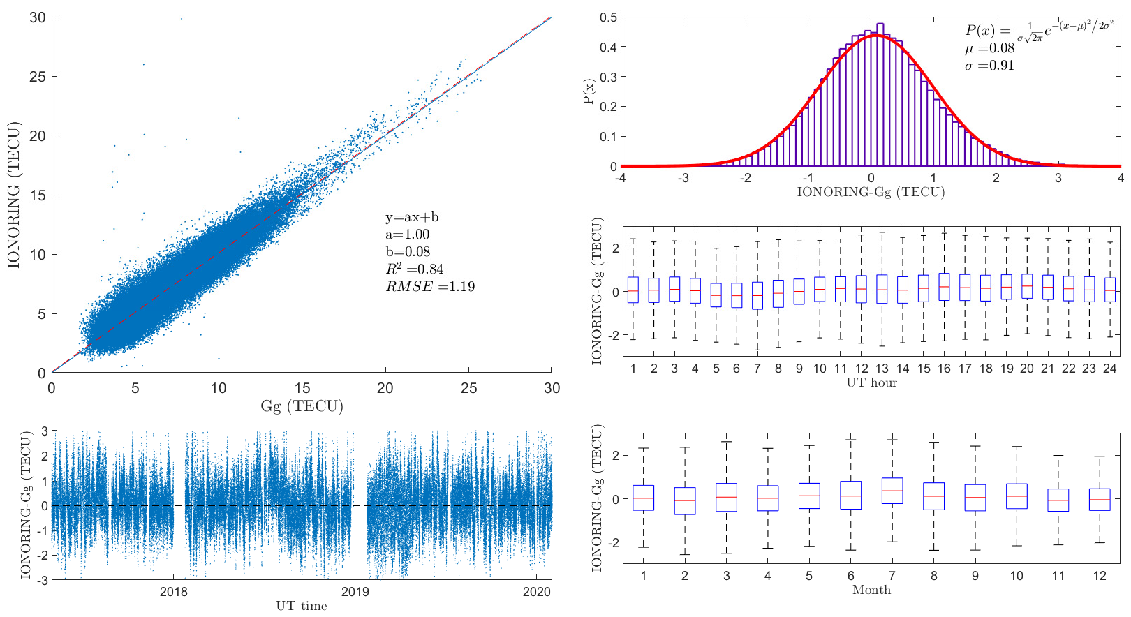
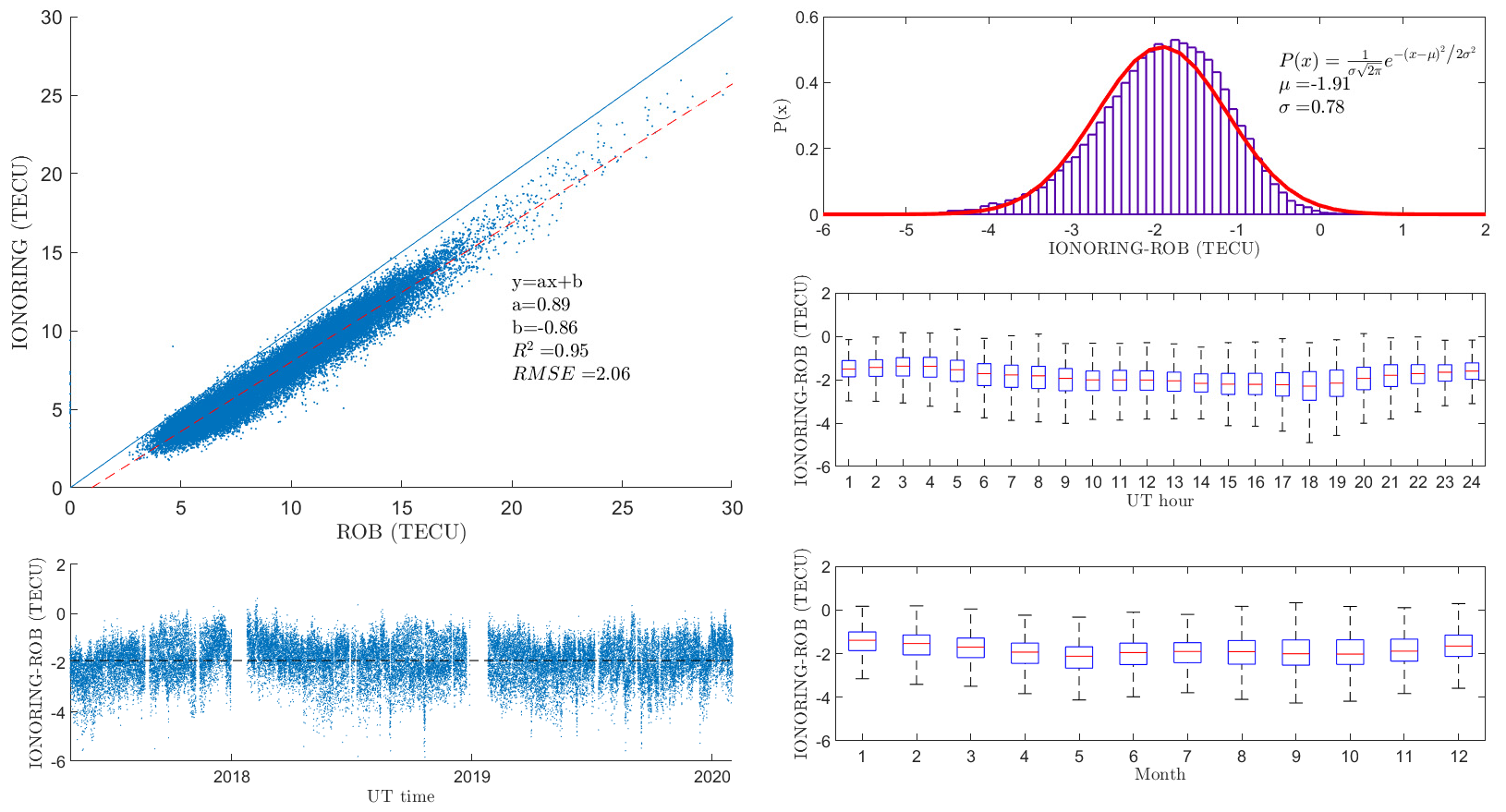
| Validation Dataset | a | b (TECu) | R2 | RMSE (TECu) | μ(TECu) | σ(TECu) |
|---|---|---|---|---|---|---|
| Gg | 1.00 | 0.08 | 0.84 | 1.2 | 0.1 | 0.9 |
| ROB | 0.89 | −0.86 | 0.95 | 2.0 | −1.9 | 0.8 |
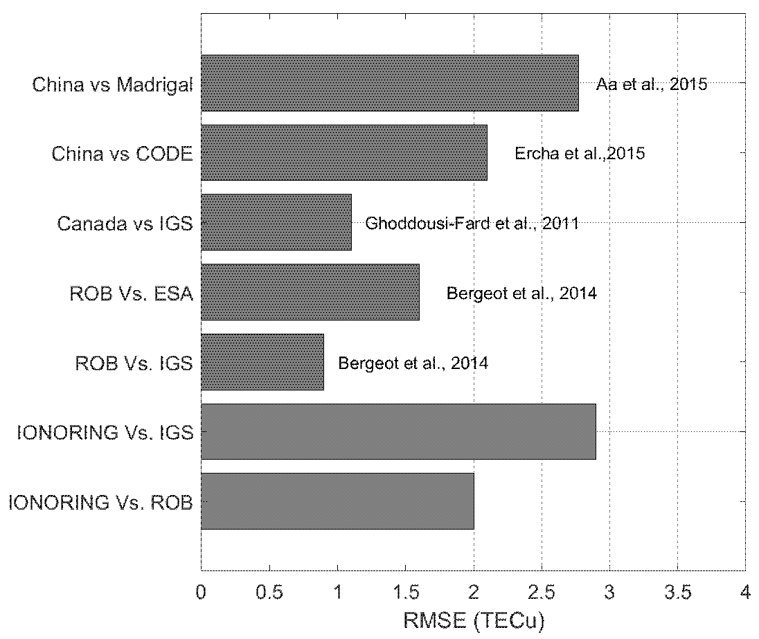
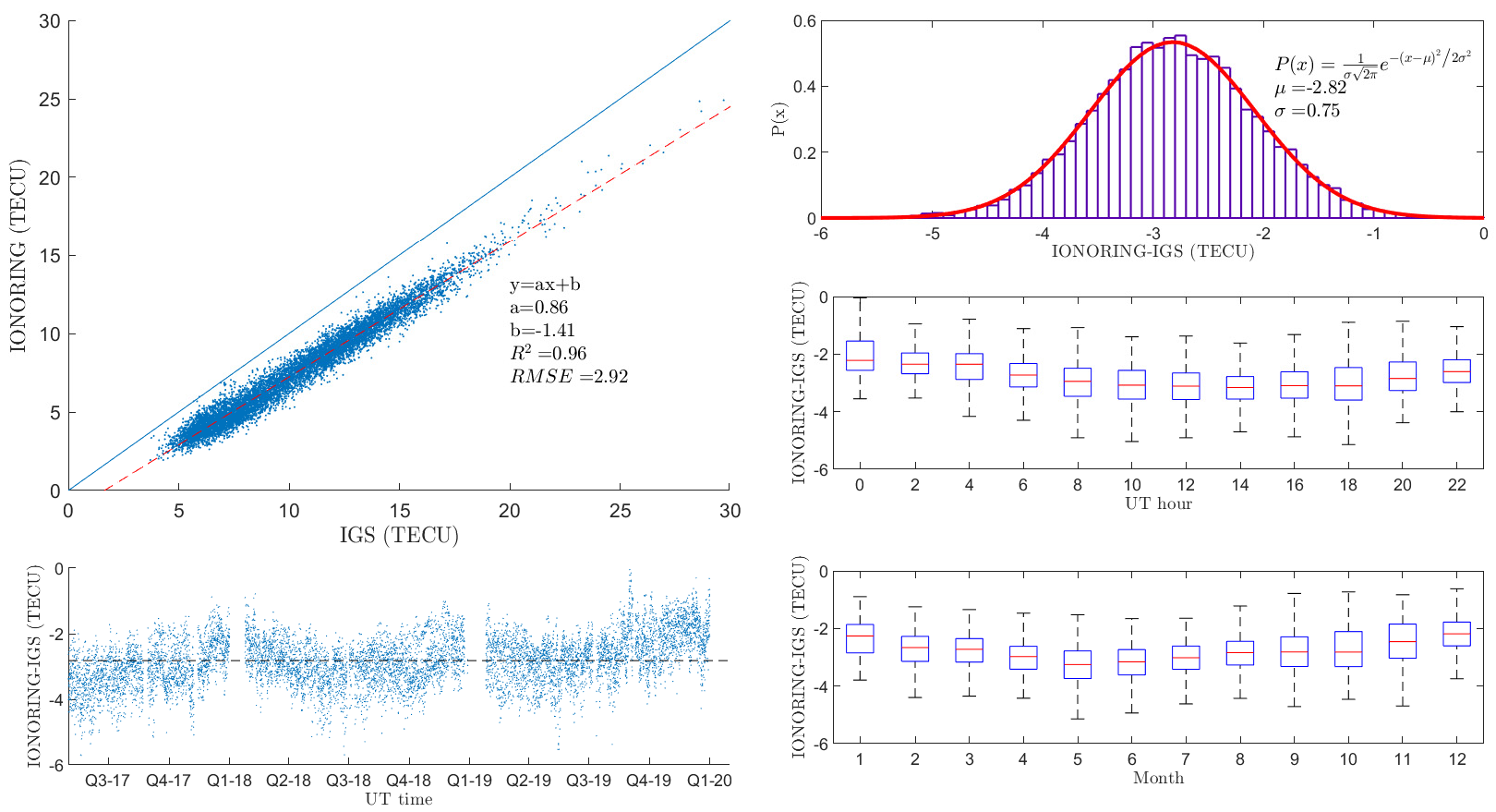
| IGS | 0.86 | −1.41 | 0.96 | 2.9 | −2.8 | 0.8 |
| Date | KLOBUCHAR | GIM | IONORING | ||||||||
|---|---|---|---|---|---|---|---|---|---|---|---|
| North (m) | East (m) | HPE (m) | North (m) | East (m) | HPE (m) | IR | North (m) | East (m) | HPE (m) | IR | |
| 25 Sep 2017 | 1.25 | 1.29 | 3.23 | 0.51 | 0.85 | 0.98 | 91% | 0.76 | 1.49 | 2.8 | 25% |
| 6 Sep 2017 | 1.04 | 1.79 | 4.29 | 0.9 | 1.74 | 3.84 | 20% | 0.75 | 1.38 | 2.47 | 67% |
Publisher’s Note: MDPI stays neutral with regard to jurisdictional claims in published maps and institutional affiliations. |
© 2021 by the authors. Licensee MDPI, Basel, Switzerland. This article is an open access article distributed under the terms and conditions of the Creative Commons Attribution (CC BY) license (https://creativecommons.org/licenses/by/4.0/).
Share and Cite
Cesaroni, C.; Spogli, L.; De Franceschi, G. IONORING: Real-Time Monitoring of the Total Electron Content over Italy. Remote Sens. 2021, 13, 3290. https://doi.org/10.3390/rs13163290
Cesaroni C, Spogli L, De Franceschi G. IONORING: Real-Time Monitoring of the Total Electron Content over Italy. Remote Sensing. 2021; 13(16):3290. https://doi.org/10.3390/rs13163290
Chicago/Turabian StyleCesaroni, Claudio, Luca Spogli, and Giorgiana De Franceschi. 2021. "IONORING: Real-Time Monitoring of the Total Electron Content over Italy" Remote Sensing 13, no. 16: 3290. https://doi.org/10.3390/rs13163290
APA StyleCesaroni, C., Spogli, L., & De Franceschi, G. (2021). IONORING: Real-Time Monitoring of the Total Electron Content over Italy. Remote Sensing, 13(16), 3290. https://doi.org/10.3390/rs13163290