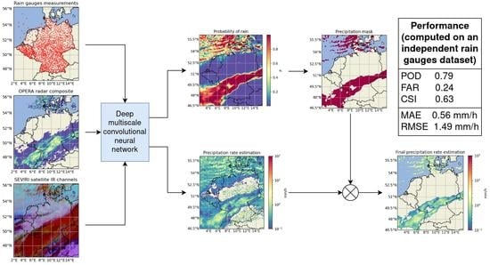
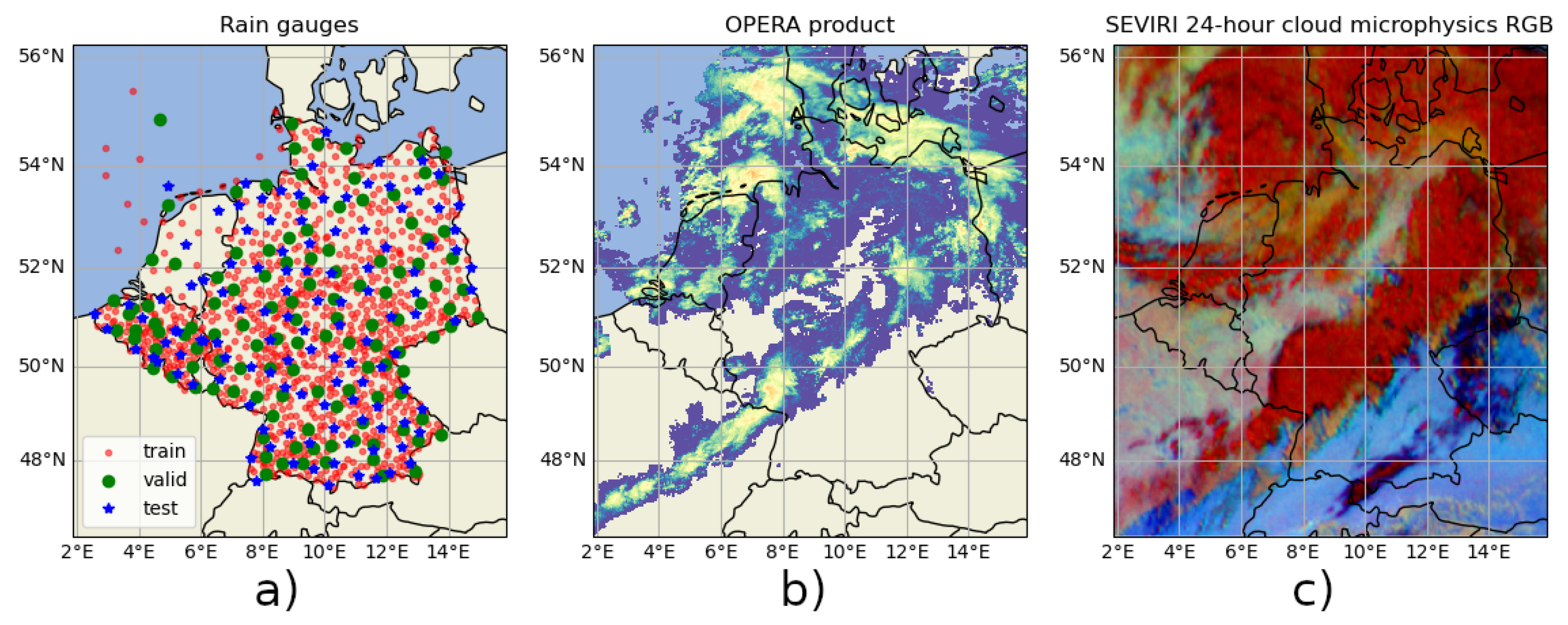
Figure 1.
Visualization of the three modalities of data source used as input, and also target for the rain gauges (a). The OPERA rain rate composite (b) and the SEVIRI 24-h cloud microphysics RGB (c) images are from 29 September 2019 12:55:00.
Figure 1.
Visualization of the three modalities of data source used as input, and also target for the rain gauges (a). The OPERA rain rate composite (b) and the SEVIRI 24-h cloud microphysics RGB (c) images are from 29 September 2019 12:55:00.
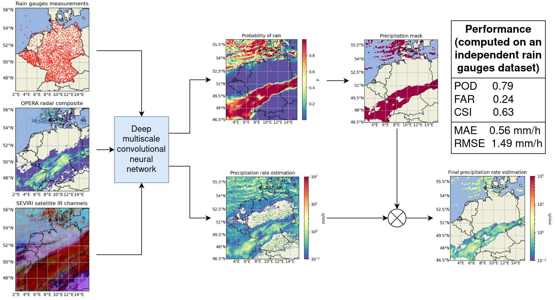
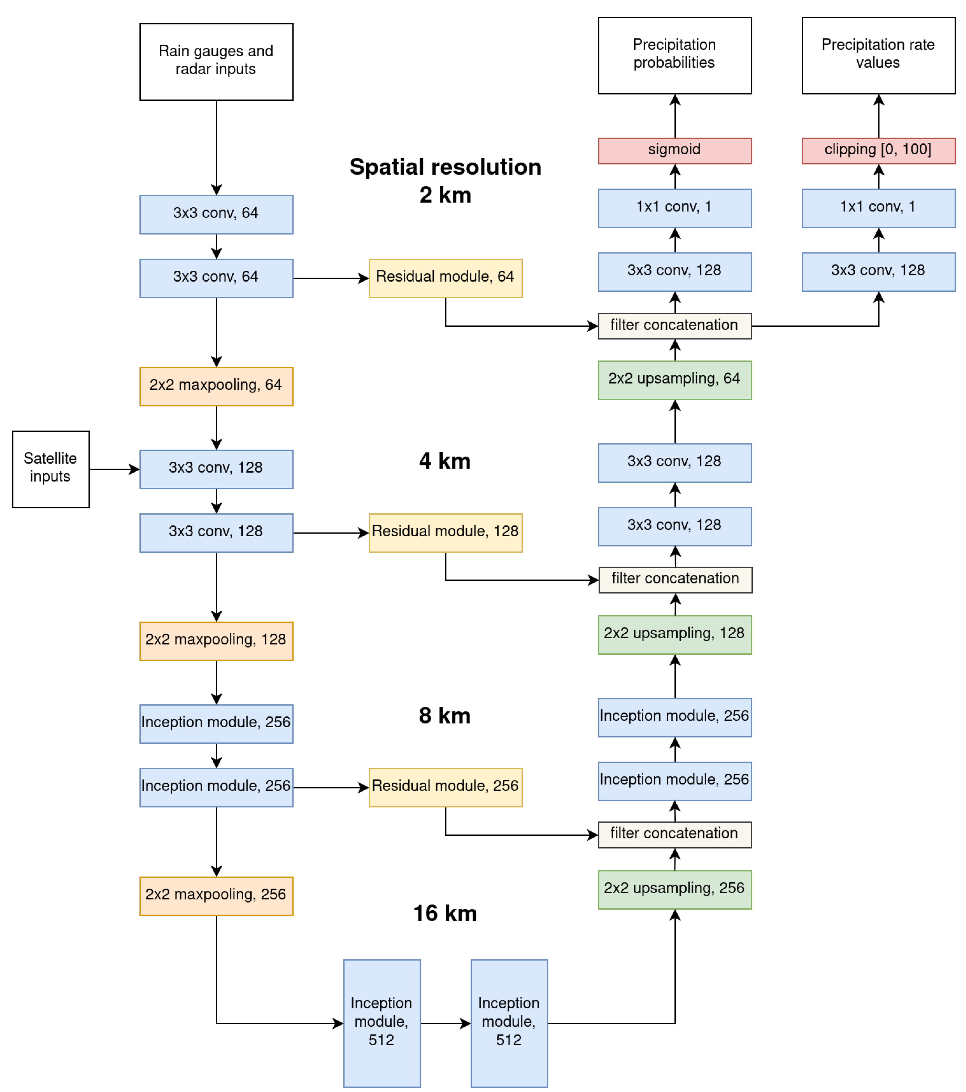
Figure 2.
The architecture of our multiscale convolutional model. Each block defines the type of layer and number of filters.
Figure 2.
The architecture of our multiscale convolutional model. Each block defines the type of layer and number of filters.
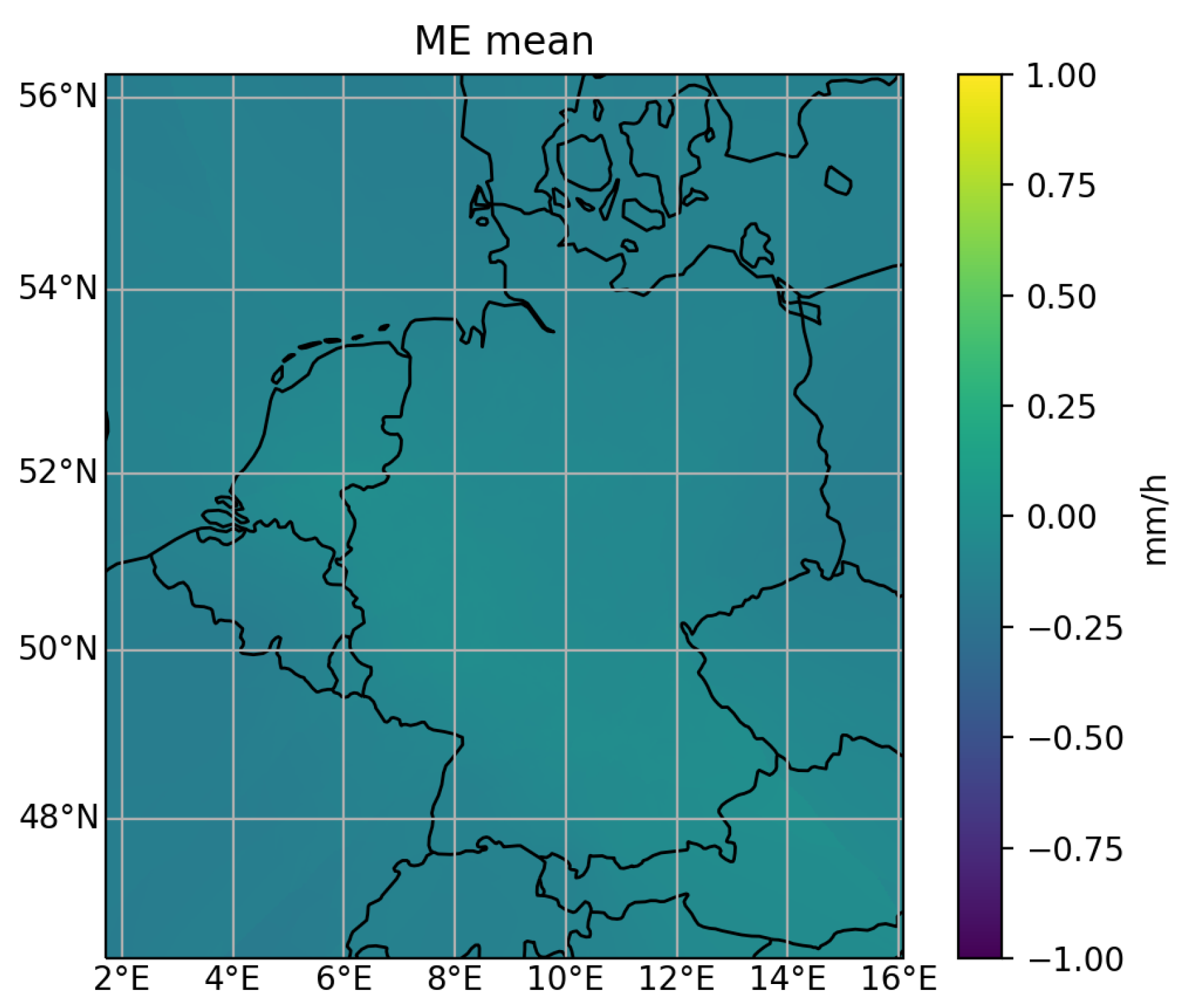
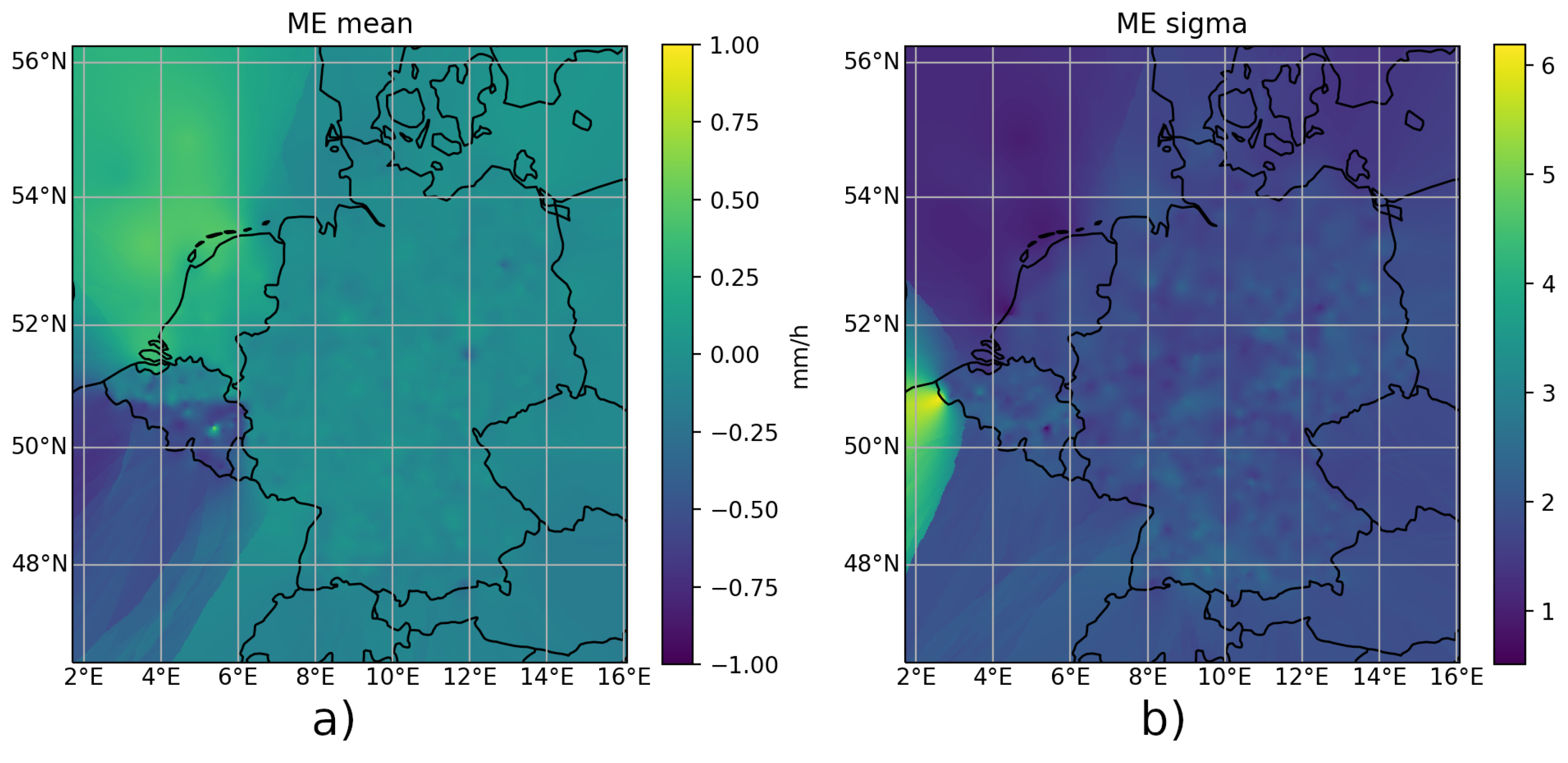
Figure 3.
Map of the average ME (a), and the standard deviation of the ME (b), for the estimation of the satellite model trained on the DWD network. The map is interpolated from the ME mean and standard deviation values of every rain gauge used in our study.
Figure 3.
Map of the average ME (a), and the standard deviation of the ME (b), for the estimation of the satellite model trained on the DWD network. The map is interpolated from the ME mean and standard deviation values of every rain gauge used in our study.
Figure 4.
Map of the average ME for the satellite model trained on the DWD network, using our bias correction method.
Figure 4.
Map of the average ME for the satellite model trained on the DWD network, using our bias correction method.
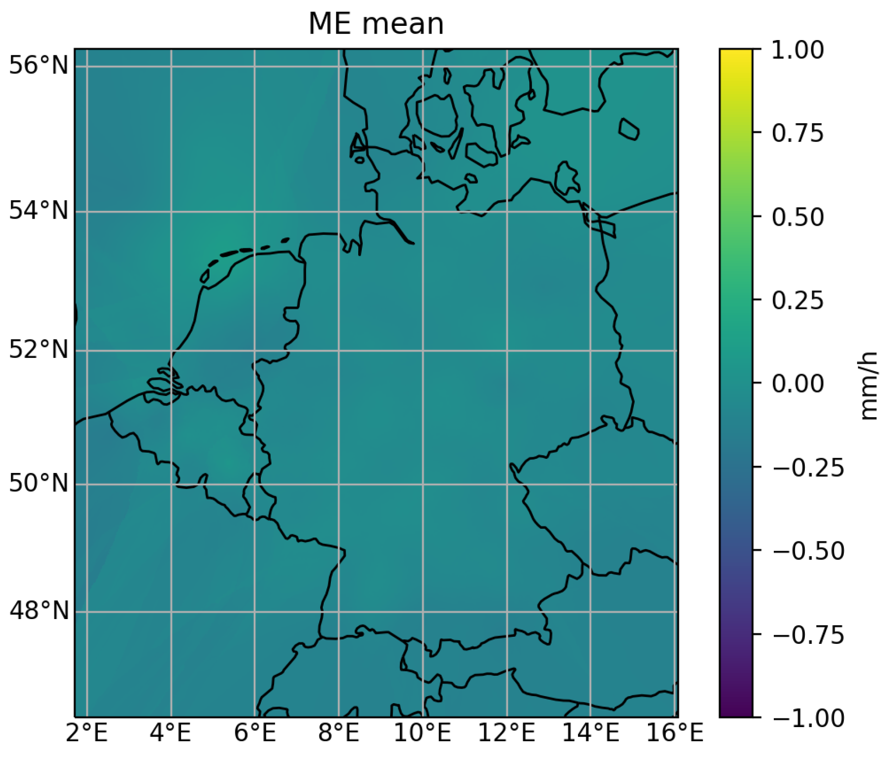
Figure 5.
Map of the average ME, for the model using the three modalities of data (satellite, radar and rain gauges), using our bias correction method.
Figure 5.
Map of the average ME, for the model using the three modalities of data (satellite, radar and rain gauges), using our bias correction method.
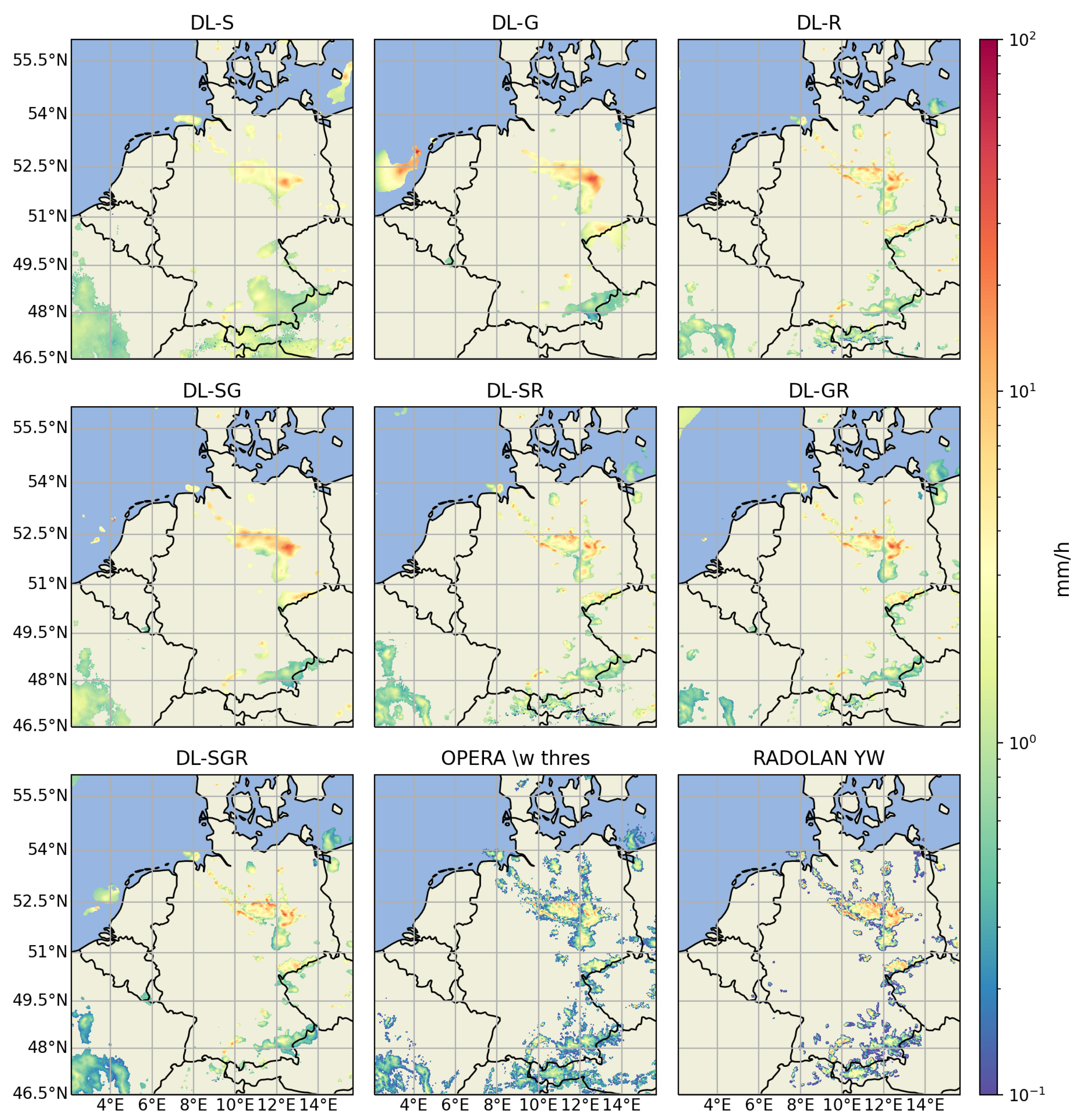
Figure 6.
The estimation map made by our model with each different combinations of the three modalities, and the rain rate map of OPERA with a minimum rain rate value thresholding, and the RADOLAN YW product, for 31 May 2016 17:40.
Figure 6.
The estimation map made by our model with each different combinations of the three modalities, and the rain rate map of OPERA with a minimum rain rate value thresholding, and the RADOLAN YW product, for 31 May 2016 17:40.
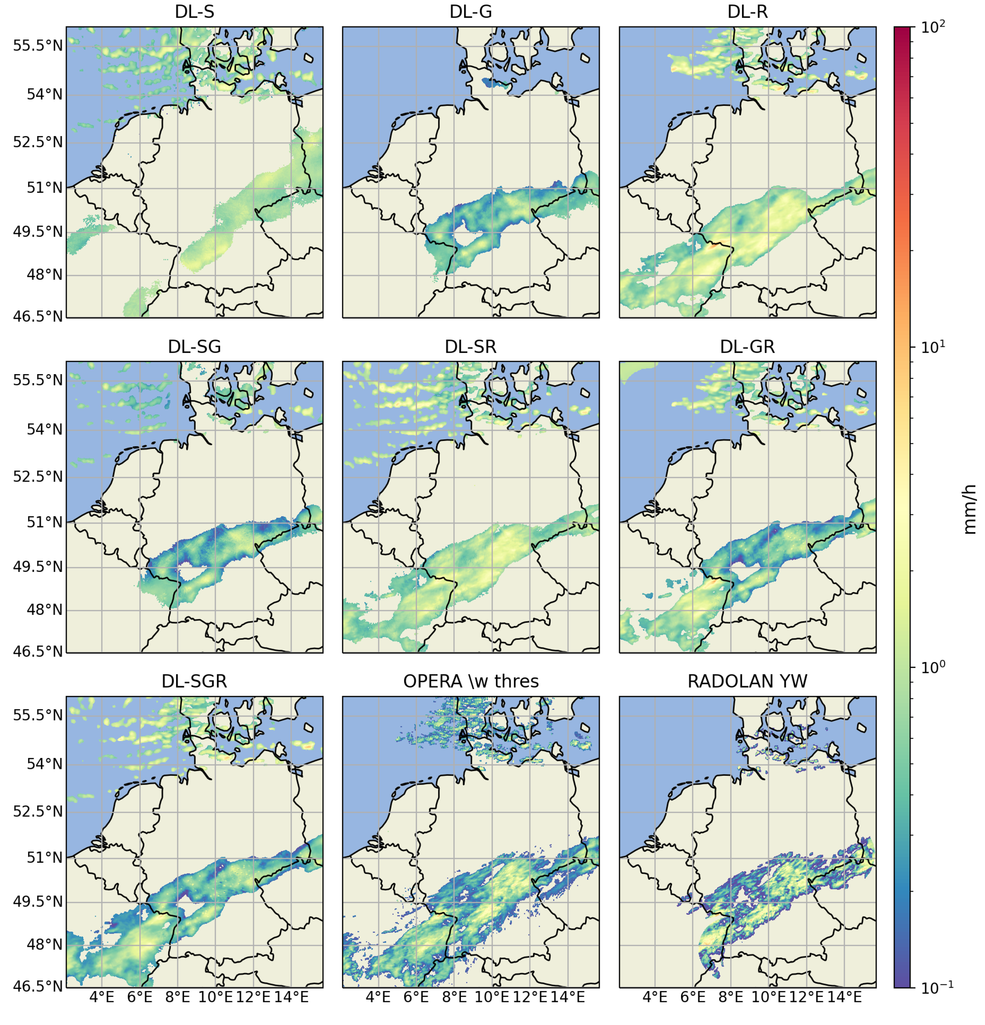
Figure 7.
The estimation map made by our model with each different combinations of the three modalities, and the rain rate map of OPERA with a minimum rain rate value thresholding, and the RADOLAN YW product, for 27 October 2019 17:25.
Figure 7.
The estimation map made by our model with each different combinations of the three modalities, and the rain rate map of OPERA with a minimum rain rate value thresholding, and the RADOLAN YW product, for 27 October 2019 17:25.
Table 1.
The test ME (in mm/h) for each network of rain gauges for the rain estimates produced by the model when using the three modalities of data (satellite, radar and rain gauges) using the non-null rain rate values. As a reference, the mean rain rate of the test rain gauges for the non-null measurements is 0.988 mm/h.
| | RMIB | SPW | VMM | KNMI (Land) | KNMI (Sea) | DWD |
|---|
| ME mean | −0.191 | −0.442 | −0.154 | 0.177 | 0.203 | −0.074 |
Table 2.
The test ME (in mm/h) for each network of rain gauges for the rain estimates produced by the model when using only the satellite modality and trained only on the DWD network of rain gauges.
Table 2.
The test ME (in mm/h) for each network of rain gauges for the rain estimates produced by the model when using only the satellite modality and trained only on the DWD network of rain gauges.
| | RMIB | SPW | VMM | KNMI (Land) | KNMI (Sea) | DWD |
|---|
| ME mean | −0.330 | −0.581 | −0.121 | 0.307 | 0.378 | −0.089 |
Table 3.
The values of the rain gauge measurements rescaling factors for each network.
Table 3.
The values of the rain gauge measurements rescaling factors for each network.
| | RMIB | SPW | VMM | KNMI (Land) | KNMI (Sea) | DWD |
|---|
| 0.809 | 0.641 | 0.861 | 1.372 | 1.819 | 0.941 |
Table 4.
The test ME (in mm/h) of each network of rain gauges, for the model using the three modalities of data (satellite, radar and rain gauges), using our bias correction method.
Table 4.
The test ME (in mm/h) of each network of rain gauges, for the model using the three modalities of data (satellite, radar and rain gauges), using our bias correction method.
| | RMIB | SPW | VMM | KNMI (Land) | KNMI (Sea) | DWD |
|---|
| ME mean | −0.154 | −0.069 | −0.001 | 0.218 | 0.077 | −0.017 |
Table 5.
The classification scores equation, value range and optimum value. The F1 score is calculated from the precision P and the recall R.
Table 5.
The classification scores equation, value range and optimum value. The F1 score is calculated from the precision P and the recall R.
| | Equation | Range | Optimum |
|---|
| POD | | [0, 1] | 1 |
| FAR | | [0, 1] | 0 |
| POFD | | [0, 1] | 0 |
| ACC | | [0, 1] | 1 |
| CSI | | [0, 1] | 1 |
| F1 | with , | [0, 1] | 1 |
Table 6.
Contingency table between the observations and the estimations, recording the number of true negatives , the number of false negatives , the number of false positives and the number of true positives .
Table 6.
Contingency table between the observations and the estimations, recording the number of true negatives , the number of false negatives , the number of false positives and the number of true positives .
| | | Observations |
|---|
| | | r = 0 | r > 0 |
|---|
| Estimations | r = 0 | | |
| r > 0 | | |
Table 7.
The regression scores equation, value range and optimum value. is an observation and is its estimation.
Table 7.
The regression scores equation, value range and optimum value. is an observation and is its estimation.
| | Equation | Range | Optimum |
|---|
| ME | | [] | 0 |
| MAE | | [] | 0 |
| RMSE | | [] | 0 |
| RV | with | [, 1] | 1 |
| PCORR | | [−1, 1] | 1 |
Table 8.
Classification scores averaged on the automatic test stations.
Table 8.
Classification scores averaged on the automatic test stations.
| | DL-S | DL-G | DL-R | DL-SG | DL-SR | DL-GR | DL-SGR |
|---|
| POD | 0.578 | 0.674 | 0.700 | 0.693 | 0.724 | 0.776 | 0.788 |
| FAR | 0.532 | 0.244 | 0.286 | 0.233 | 0.287 | 0.235 | 0.243 |
| POFD | 0.058 | 0.019 | 0.025 | 0.018 | 0.025 | 0.021 | 0.022 |
| ACC | 0.914 | 0.957 | 0.954 | 0.959 | 0.956 | 0.964 | 0.964 |
| CSI | 0.347 | 0.554 | 0.541 | 0.572 | 0.559 | 0.627 | 0.629 |
| F1 | 0.513 | 0.711 | 0.701 | 0.726 | 0.716 | 0.769 | 0.771 |
Table 9.
Regression scores averaged on the automatic test stations. The ME, the MAE and the RMSE are expressed in mm/h.
Table 9.
Regression scores averaged on the automatic test stations. The ME, the MAE and the RMSE are expressed in mm/h.
| | DL-S | DL-G | DL-R | DL-SG | DL-SR | DL-GR | DL-SGR |
|---|
| ME | −0.170 | −0.095 | 0.109 | −0.065 | 0.059 | 0.034 | −0.082 |
| MAE | 0.776 | 0.659 | 0.688 | 0.653 | 0.663 | 0.590 | 0.557 |
| RMSE | 1.846 | 1.759 | 1.611 | 1.704 | 1.589 | 1.516 | 1.488 |
| RV | 0.141 | 0.244 | 0.340 | 0.271 | 0.359 | 0.418 | 0.445 |
| PCORR | 0.433 | 0.504 | 0.637 | 0.554 | 0.634 | 0.683 | 0.688 |
Table 10.
Classification scores comparison between OPERA and our DL-R and DL-SGR models.
Table 10.
Classification scores comparison between OPERA and our DL-R and DL-SGR models.
| | OPERA | DL-R | DL-SGR |
|---|
| POD | 0.604 | 0.700 | 0.788 |
| FAR | 0.407 | 0.286 | 0.243 |
| POFD | 0.037 | 0.025 | 0.022 |
| ACC | 0.934 | 0.954 | 0.964 |
| CSI | 0.422 | 0.541 | 0.629 |
| F1 | 0.590 | 0.701 | 0.771 |
Table 11.
Regression scores comparison between OPERA and our DL-R and DL-SGR models. The ME, the MAE and the RMSE are expressed in mm/h.
Table 11.
Regression scores comparison between OPERA and our DL-R and DL-SGR models. The ME, the MAE and the RMSE are expressed in mm/h.
| | OPERA | DL-R | DL-SGR |
|---|
| ME | −0.428 | 0.109 | −0.082 |
| MAE | 0.721 | 0.688 | 0.557 |
| RMSE | 1.872 | 1.611 | 1.488 |
| RV | 0.055 | 0.340 | 0.445 |
| PCORR | 0.505 | 0.637 | 0.688 |
Table 12.
Classification scores comparison between RADOLAN YW and our DL-SGR model on the automatic test stations from the DWD network.
Table 12.
Classification scores comparison between RADOLAN YW and our DL-SGR model on the automatic test stations from the DWD network.
| | DL-SGR | RADOLAN YW |
|---|
| POD | 0.905 | 0.545 |
| FAR | 0.109 | 0.319 |
| POFD | 0.011 | 0.022 |
| ACC | 0.983 | 0.942 |
| CSI | 0.818 | 0.432 |
| F1 | 0.897 | 0.598 |
Table 13.
Regression scores comparison between RADOLAN YW and our DL-SGR model on the automatic test stations from the DWD network. The ME, the MAE and the RMSE are expressed in mm/h.
Table 13.
Regression scores comparison between RADOLAN YW and our DL-SGR model on the automatic test stations from the DWD network. The ME, the MAE and the RMSE are expressed in mm/h.
| | DL-SGR | RADOLAN YW |
|---|
| ME | 0.140 | −0.207 |
| MAE | 0.395 | 0.722 |
| RMSE | 1.140 | 1.788 |
| RV | 0.639 | 0.012 |
| PCORR | 0.885 | 0.566 |
Table 14.
RMSE statistics (the standard deviation, the mean and the standard deviation normalized by the mean) across all test stations.
Table 14.
RMSE statistics (the standard deviation, the mean and the standard deviation normalized by the mean) across all test stations.
| | DL-S | DL-G | DL-R | DL-SG | DL-SR | DL-GR | DL-SGR |
|---|
| std | 0.104 | 0.110 | 0.093 | 0.103 | 0.089 | 0.088 | 0.084 |
| mean | 0.834 | 0.679 | 0.715 | 0.679 | 0.684 | 0.604 | 0.576 |
| std/mean | 0.125 | 0.162 | 0.130 | 0.152 | 0.130 | 0.145 | 0.146 |
Table 15.
Classification and regression scores comparison between the different networks of rain gauges for the DL-S model. The ME, the MAE and the RMSE are expressed in mm/h.
Table 15.
Classification and regression scores comparison between the different networks of rain gauges for the DL-S model. The ME, the MAE and the RMSE are expressed in mm/h.
| | KNMI (Sea) | KNMI (Land) | RMIB | SPW | VMM | DWD |
|---|
| POD | 0.575 | 0.549 | 0.501 | 0.515 | 0.495 | 0.597 |
| FAR | 0.454 | 0.423 | 0.520 | 0.620 | 0.527 | 0.526 |
| POFD | 0.077 | 0.055 | 0.056 | 0.053 | 0.043 | 0.057 |
| ACC | 0.872 | 0.898 | 0.904 | 0.922 | 0.925 | 0.917 |
| CSI | 0.387 | 0.389 | 0.324 | 0.280 | 0.315 | 0.359 |
| F1 | 0.557 | 0.560 | 0.489 | 0.436 | 0.478 | 0.526 |
| ME | −0.337 | −0.062 | −0.309 | −0.205 | −0.149 | −0.198 |
| MAE | 1.173 | 0.844 | 0.705 | 0.715 | 0.829 | 0.774 |
| RMSE | 3.639 | 1.705 | 2.127 | 1.713 | 1.852 | 1.859 |
| RV | 0.111 | 0.189 | 0.200 | −0.021 | 0.200 | 0.136 |
| PCORR | 0.352 | 0.454 | 0.478 | 0.375 | 0.479 | 0.438 |
Table 16.
Performance results for the daily precipitation accumulation estimation, measured on the climatological rain gauges measurements at the test dates. The ME, the MAE and the RMSE are expressed in mm.
Table 16.
Performance results for the daily precipitation accumulation estimation, measured on the climatological rain gauges measurements at the test dates. The ME, the MAE and the RMSE are expressed in mm.
| | OPERA | DL-S | DL-G | DL-R | DL-SG | DL-SR | DL-GR | DL-SGR |
|---|
| ME | −0.614 | −0.111 | −0.589 | −0.411 | −0.519 | −0.182 | −0.452 | −0.536 |
| MAE | 1.351 | 1.314 | 0.905 | 0.984 | 0.868 | 0.915 | 0.817 | 0.829 |
| RMSE | 2.893 | 2.720 | 2.292 | 2.232 | 2.041 | 2.067 | 1.910 | 1.944 |
| RV | 0.386 | 0.488 | 0.450 | 0.665 | 0.710 | 0.708 | 0.747 | 0.739 |
| PCORR | 0.743 | 0.735 | 0.868 | 0.840 | 0.878 | 0.856 | 0.899 | 0.901 |
Table 17.
Performance results for the daily precipitation accumulation estimation with bias correction, measured on the climatological rain gauges measurements at the test dates. The ME, the MAE and the RMSE are expressed in mm.
Table 17.
Performance results for the daily precipitation accumulation estimation with bias correction, measured on the climatological rain gauges measurements at the test dates. The ME, the MAE and the RMSE are expressed in mm.
| | OPERA | DL-S | DL-G | DL-R | DL-SG | DL-SR | DL-GR | DL-SGR |
|---|
| ME | −0.012 | −0.104 | −0.044 | −0.154 | −0.031 | −0.139 | −0.066 | −0.067 |
| MAE | 1.376 | 1.316 | 0.893 | 0.996 | 0.857 | 0.918 | 0.789 | 0.788 |
| RMSE | 2.872 | 2.723 | 2.270 | 2.211 | 2.045 | 2.066 | 1.830 | 1.826 |
| RV | 0.287 | 0.487 | 0.251 | 0.667 | 0.699 | 0.707 | 0.757 | 0.762 |
| PCORR | 0.743 | 0.735 | 0.868 | 0.840 | 0.878 | 0.856 | 0.899 | 0.901 |


