Abstract
Habitat degradation, mostly caused by human impact, is one of the key drivers of biodiversity loss. This is a global problem, causing a decline in the number of pollinators, such as hoverflies. In the process of digitalizing ecological studies in Serbia, remote-sensing-based land cover classification has become a key component for both current and future research. Object-based land cover classification, using machine learning algorithms of very high resolution (VHR) imagery acquired by an unmanned aerial vehicle (UAV) was carried out in three different study sites on Mt. Stara Planina, Eastern Serbia. UAV land cover classified maps with seven land cover classes (trees, shrubs, meadows, road, water, agricultural land, and forest patches) were studied. Moreover, three different classification algorithms—support vector machine (SVM), random forest (RF), and k-NN (k-nearest neighbors)—were compared. This study shows that the random forest classifier performs better with respect to the other classifiers in all three study sites, with overall accuracy values ranging from 0.87 to 0.96. The overall results are robust to changes in labeling ground truth subsets. The obtained UAV land cover classified maps were compared with the Map of the Natural Vegetation of Europe (EPNV) and used to quantify habitat degradation and assess hoverfly species richness. It was concluded that the percentage of habitat degradation is primarily caused by anthropogenic pressure, thus affecting the richness of hoverfly species in the study sites. In order to enable research reproducibility, the datasets used in this study are made available in a public repository.
1. Introduction
1.1. General Overview and Objectives of the Study
The fundamental goal of ecology has always been to maintain a high level of biodiversity. In order to fully comprehend the way an ecosystem functions, it must be understood how dependent species are on ecological resources as their only source of survival, including, but certainly not limited to, the importance of gradual changes in habitat properties and land coverage. The habitat condition is a set of influences acting on the natural distribution, structure, and functions of its typical species survival. A precise estimation of the habitat condition for a biodiversity assessment with limited field observations presents a great challenge for remote sensing [1]. Nonetheless, a comprehensive knowledge of the habitat condition of a species’ requirements is essential in improving conservation actions and policies [1,2].
As habitat degradation and landscape modification are one of the key drivers of biodiversity loss, it is of utmost importance that ecological studies are conducted at a fine scale resolution [3,4]. To date, technologies of remote sensing and photogrammetry have both huge potential and profitable results when it comes to different environmental [5,6], agricultural [7], and land use [8] research. In order to support resource management surveys and inventories, as well as to develop better and more relevant vegetation mapping applications that could serve as a model for displaying local habitat characteristics of species, there is an evident need for the classification of land cover maps to be more precise [9,10]. One of the most useful and reliable ways to monitor an ecosystem’s land coverage is through land cover maps, which indicate different types (classes) of the Earth’s surface (e.g. forests, rivers, wetlands, etc.). Accurate land cover maps that can detect and track transitions of the land surface over a period of time are required for science, monitoring, and reporting [11].
However, not every remote sensing instrument has been able to provide high-resolution data that meet the requirements of spatial ecology. Unmanned aerial vehicles (UAVs) have become one of the most promising toolkits for ecological studies capturing landscape habitats from a bird’s eye view [12,13,14,15,16,17]. Compared to satellite techniques, the advantage of these systems is their ability to deliver data quickly in a very high spatial and temporal resolution. The short time required for launching and possibility for frequent surveys, as well as its fast data acquisition and transmission, encourage the practice of analyzing small-sized and medium-sized fields and complex ecosystems [6,10,18,19].
There are various sources of widely used high-resolution maps, such as the pan-European high-resolution layers, that indicate specific land cover characteristics [20]; however, none of them show vegetation types in their original natural form, such as the Map of the Natural Vegetation of Europe (EPNV), compiled and produced by an international team of vegetation scientists from 31 European countries over the period of 1979–2003 [21]. This source was used for information on the potential distribution of the dominant natural plant communities.
Habitat degradation represents a slow and often subtle deterioration in habitat condition caused by natural processes and human activities [22]. Habitat degradation, due to agricultural intensification and urbanization, is a global problem that entails, among other things, a decline in the number of pollinators [23,24,25,26,27]. The pollinator decline results in the lack of pollination services having a negative impact on the plant diversity maintenance and ecosystem stability. Regarding the pollinators referred to in this study, hoverflies are the most biologically diverse families of Diptera [28], and the most important pollinators besides bees [28,29,30]. As bioindicators of the ecosystem’s condition [29], hoverflies serve as valuable model organisms in studies on both climate change and the change in landscape structure and land use [26,27,28,31,32,33]. Hoverflies occupy a wide variety of habitats, aside from extreme conditions, such as dry areas and frozen landscapes [29,30,34]. The hoverfly larvae can be found in a broad range of land cover types, whereas the adults are mostly found in areas with flowers. In general, hoverfly diversity is higher in habitats connected to mountainous forested areas, and lower in shrub, grass, open, and agricultural areas [26,34,35]. The mobility of hoverflies varies considerably, ranging from low level flyers, which fly less than 2 m per day, to highly mobile migratory species that exceed 2 km per day. Nonetheless, over 90% of the hoverflies are considered to be non-migratory species [28,36], which makes the UAV measurements scale appropriate for a hoverfly habitat condition assessment.
Publicly available datasets are important when tracking ecological changes, changes in land cover, and its effects on species [37]. In order for UAV to become a standard toolkit for conservation ecologists, publicly available datasets and reproducible data processing workflows are needed. Considering all of the above mentioned, a new method was developed for the quantification of habitat degradation linked to the species richness of hoverflies, with the following objectives:
- Obtain very high resolution (VHR) land cover maps in three study sites using UAV acquired imagery and the framework proposed by De Luca et al [38];
- Determine the hoverfly habitat degradation coverage in the three designated study sites using precise land cover classification and biodiversity expert knowledge;
- Compare corresponding habitat degradation coverage with the difference in potential and recent richness of hoverfly species in three study sites and evaluate its utility for the habitat condition assessment;
- Provide guidance in a state-of-the art remote sensing toolbox specifically targeting research in spatial and landscape ecology that requires such tools. Data processing workflows are also available in the form of free tutorials for researchers interested in replicating the study or using the same/similar experimental settings, providing research reproducibility.
1.2. Background
Nowadays, the ecology community is relying on newer technologies to complete its goals of detailed land cover analysis: (UAVs). Recently, a growing number of studies have focused on using UAVs for land cover classification [8,16,38,39,40,41,42,43]. However, most image classification methods rely on pixel-based techniques that have limitations when it comes to high-resolution satellite data and UAV imagery [16,43,44]. With the emergence of VHR images, the possibility for classifying land cover types at more itemized levels has become available. Containing high intra-class spectral variability, features in VHR images can be easily separated based on spatial, textural, and contextual information [43]. Taking this into consideration, pixel-based image classification is replaced with object-based image analysis (OBIA), a new approach for managing spectral variability. In order to reduce the intra-class spectral variability, OBIA works with groups of homogenous and contiguous pixels (also called geographical objects; segments) with similar information to base units in order to conduct the classification. OBIA involves both spectral and spatial information for the classification and categorization of pixels based on their shape, texture, and spatial relationship with the surrounding pixels [16,43,44,45,46]. In order to perform OBIA, two steps are required: image segmentation and image classification [47]. Since this method implies obtaining geographic information from remote sensing imagery analysis, the new term GEOBIA (Geographic Object-Based Image Analysis) was introduced [48,49]. According to Hay and Castilla 2008, GEOBIA is a sub-discipline of geographic information science (GIScience), which is devoted to developing an automated method for image censoring and analysis.
De Luca et al. (2019) demonstrated an exceptional achievement in classification accuracy of object-based land cover cork oak woodlands using UAV imagery and an open-source software workflow [38]. They compared two machine learning classifiers on a small portion of the captured study area that can be applicable to the whole study site [38]. Other researchers highlighted the importance of UAV multispectral camera and platform capabilities to obtain more accurate results [39]. Natesan et al. (2017) used the lightweight UAV spectrometer spectral exposure labeled ground point to determine land cover classification [41]. Kalantar et al. (2017) presented a method that integrates the fuzzy unordered rule induction algorithm (FURIA) into OBIA to achieve accurate land cover extraction from UAV images [43]. Horning et al. (2020) tested image classification algorithms on UAV images obtained at different heights in two different open-source software [16]. Al-Najjar et al. (2019) applied convolutional neural networks (CNNs) to a fused digital surface model (DSM) and UAV datasets for land cover classification [50]. Ventura et al. (2018) showed the potential of UAVs in coastal monitoring by evaluating the suitability of georeferenced orthomosaics and OBIA in detecting and classifying coastal features [51].
To date, the EPNV map has been used only for botanical purposes and estimations, such as the ecological classification of Europe [52], nature conservation purposes [53], and gap analysis [54]. Thereafter, the EPNV was applied for the classification of ecological areas at different scales and the production and use of detailed maps of regions and countries. It was also used as a baseline for estimating the natural potential in Germany [55] and the Caucasus [52], reconstructing ancient vegetation [56], and for dividing European hoverfly species according to their habitat preferences [57].
Several studies have used UAVs for detecting [58], monitoring [59], and sampling [60] insect species, but, reportedly, no previous study has been conducted using EPNV or UAV classified land cover maps to draw similar conclusions regarding any group of insects. It is known that VHR UAV images are not simple to acquire and process. Additionally, domain knowledge is required when processing images with multiple classes, and the robustness of the methodology needs to be addressed. Numerous works have used UAV–OBIA for the classification of different environments [38,43,51,61,62,63,64,65,66]. Among them, several studies provided a new methodology for quantifying habitat properties [51,66]; however, none of them made similar attempts to determine habitat degradation derived from land cover classification that has an impact on hoverfly species richness.
2. Materials and Methods
2.1. Study Sites
The area of Mt. Stara Planina belongs to the Carpatho-Balkanids. The geological structure of Mt. Stara Planina shows that various morphological processes occurred under the influence of endogenous and exogenous forces: primarily fluvial and karstic erosion that led to the formation of diverse relief features that created the unique richness of landscape diversity. Regarding the aspect of habitat and species diversity, this mountain represents one of the most important and floristically and faunistically diverse parts of Serbia and the entire Balkan Peninsula [67,68].
All three study sites belong to Mt. Stara Planina (Figure 1). Two of them, geographically and spatially near to one another, Dojkinci1 (43°14′0′′ N; 22°46′50′′ E) and Dojkinci2 (43°15′33′′ N; 22°46′34′′ E), were named after a village and Dojkinačka river, which flows through this region. The third study site is a very popular and well-known peak of Stara Planina, known not only for its authentic name Babin zub (43°22′37′′ N; 22°37′33′′ E), but also for the various rock formations of coarse sandstones, located at 1.758 m above sea level. On the opposite side of this rocky mass is an environment that is under lush vegetation, which was captured by the UAV.
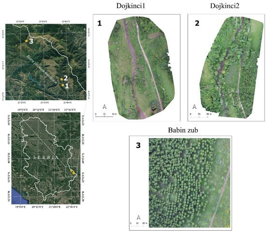
Figure 1.
The map of Serbia (left) with three study sites representing the geographical position of study areas captured by the UAV (right).
In Dojkinci1 and Dojkinci2, the dominant woody species is European beech (Fagus sylvatica). Alder (Salix) and willow (Alnus glutinosa) are found along the riverbanks, as well as examples of low vegetation, such as ferns (Pteridium aquilinum) and Petasites, which prefer moisture. Scrubland is heterogeneous and composed mostly of genus Rosa, dogwood plants (Cornus mas and Cornus sanguinea), and hawthorn (Crataegus monogyna and C. pentagyna) [67].
Babin zub is dominated by spruce (Picea abies) and fir (Abies) conifers that are spread over slopes, whereas juniper (Juniperus sibirica) is present on the clearings. Mullein (Verbascum sp.) can reach a height of up to 2 m in these areas [67].
The climate on Mt. Stara Planina is a combination of a continental climate in the north and the mountain climate of the Balkan mountain range in the south and south-east region. Summers are semi-dry, with an average July temperature of 20 °C and precipitation up to 70 mm, whereas the winters are short and mild [67,68].
Five vegetation belts are prevalent in this region: beech, oak, the Norway spruce, alpine, and subalpine. In order to protect the natural and traditional values of the region, the Serbian Government issued an official protection of Stara Planina in 1997 [67].
According to the EPNV (see in [57]), the study sites Dojkinci1 and Dojkinci2 belong to the vegetation type of beech and mixed beech forests (E), whereas the study site Babin zub contains elements of two vegetation types: alpine, subalpine, and oro-Mediterranean vegetation (A) and montane spruce and mixed spruce forests (B) [57].
2.2. Methodology, UAV Data Acquisition, and Processing Outputs
The schematic workflow of all the steps required for the overall methodology was given in Figure 2.
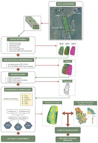
Figure 2.
Flowchart of the overall methodology.
Flowchart in Figure 2 presents the steps in the methodology: VHR images acquired by the UAV were processed and VHR land cover maps were obtained in three study sites. Afterwards, the habitat degradation coverage was determined and compared with the EPNV map. Finally, comparison of potential and recent richness of hoverfly species on three study sites was linked to percentage of habitat degradation. Habitat degradation was examined based on two aspects: one measured by the loss/presence of the hoverfly species richness and the other measured by detailed UAV assessment of land cover classes indicating degradation.
In this study the land cover classification was carried out in complex landscape areas (e.g., due to angle of the slope) located in three study sites in Eastern Serbia. Different land cover classes were derived using three machine learning algorithms. The procedure of data acquisition and the pre-processing steps were based on the work of De Luca et al. (2019). The image processing workflow is given in Figure 2. Red arrows indicate the processes summarized in bullet points, whereas the green ones represent the visualized output.
An UAV quadcopter type DJI Inspire 1 (SZ DJI Technology Co., Ltd., Shenzhen, China) with Zenmuse X3 gimbal, which can support camera replacement of RGB and NDVI (normalized difference vegetation index) modified camera, was used in this study (Table 1.) Two congruent double flight grid missions were executed at each study site with both RGB and NDVI cameras, using the Pix4Dcapture application (Pix4D S.A., Switzerland). This flight mission covered approximately 3–4 ha with a ground sampling distance (GSD) of 3–4 cm depending on the slope and terrain relief. Both missions contained the same flight parameters: altitude of 90 m, 90% of front and side overlap, and camera angle facing down at 80°. All field work data were acquired during the same day on all three study sites. Image acquisition was performed in sunny and windless conditions, when the sun was in its zenith position, in order to avoid potential shadows of high trees and shrubs.

Table 1.
Technical characteristics of DJI Inspire 1, RGB, and NDVI modified cameras.
After downloading, the images were processed in the photogrammetry software Pix4Dmapper (2021 Pix4D SA, Switzerland). The software includes three main steps: (1) initial processing, (2) point cloud and mash, and (3) digital surface model (DSM), orthomosaics, and index. NovAtel SMART6-L GNSS SMART Antenna capable of up to 2 cm real-time kinematic (RTK) precision was used and five ground control points (GCPs) were inserted for each study site in order to enhance the global accuracy of final orthomosaics.
Two orthomosaics were generated per study site. One orthomosaic was produced out of stitched images from the RGB camera and the other from an NDVI modified camera where the blue channel is replaced with an NIR channel. It is key to consider the change in the quality of the orthomosaic and area covered with a UAV once it is presented with as an obstacle for gathering quality images, such as a deep slope. The results gathered from an UAV can be limited by the slope. For example, the area coverage obtained by the camera mounted on the UAV can either be significantly increased or decreased depending on the angle of the slope. The Pix4Dmapper software itself automatically generates a DSM for each of them. Once all of the orthomosaics were gathered, initial assumptions about the ability for UAVs to manage slopes were confirmed. Although the missions were identical and applied equally for each site, the areas covered in Dojkinci1 and Dojkinci2 were approximately 4 ha, whereas on Babin zub, the area covered was around 8 ha. This difference in area coverage while performing the same mission is due to the distinction and complexity of the slope of terrains, which also influenced the result in the final output of the orthomosaic drawing errors during the processes of image segmentation and classification.
Because of the noise-affected data, especially on the borders of the orthomosaic, and in order to correctly process the images provided by the UAV, it was decided to process only one part of the generated orthomosaic for the third study site, Babin zub. A rectangular area for Babin zub, which is the central part of the orthomosaic and represents the third study site, was marked and clipped.
Further processing until the final output was performed in QGIS software (QGIS Development Team, 2020). Red, green, blue, and DSM channels were used from the RGB orthomosaic. NDVI value was calculated from the NDVI camera. Each of these bands were split and normalized to the value 0–255 and saved to 8bit. The purpose of normalization of each band to the common values is to give each layer the same importance in order to prevent and reduce the potential outliers in the segmentation process. Lastly, all five layers were merged into a final orthomosaic that represented the base of OBIA operations. This procedure was applied to all three previously mentioned study sites.
After data collection and processing outputs, the workflow can be separated into three main steps: segmentation, classification, and accuracy assessment. They were performed using plug-in OrfeoToolbox for QGIS software: an open-source state-of-the-art remote sensing project developed by the French Space Agency [69]. Its extensive base of algorithms can process high-resolution images and is accessible from different software. QGIS version 3.10.3-A Coruña and OTB 7.0 were used to perform all workflows.
2.3. Object-Based Image Detection
The object-oriented classification procedure starts with a segmentation process where the original image is subdivided into objects based on their spectral and spatial similarities [47]. The large-scale mean-shift (LSMS) segmentation algorithm became the focus of remote sensing community since being introduced by Fukunaga and Hostetler in 1975 and complemented by Commaniciu in 2002 [69]. It is not considered a real segmentation algorithm itself but a nonparametric method in which each polygon assigned to a segmented image contains the radiometric mean and variance of each band. Its application produces a labeled artifact-free vector file where pixel neighbors whose range distance is below range radius will be grouped into the same cluster [70,71]. The LSMS workflow procedure in OTB includes three consecutive steps: LSMS segmentation, LSMS small regions merging, and LSMS vectorization [71,72].
The first step is LSMS segmentation, where, on each of the merged five-layer orthomosaics, a range radius value of 3 was applied, which was carried out for all three study sites. Range radius in OTB represents the threshold of spectral signature that relies on Euclidean distance that is expressed in radiometry units in order to consider neighborhood pixels for averaging [71,72]. Range radius values from 1 to 15 were tested. Changing values of the range radius leads to the difference in numbers and sizes of segments corresponding to different objects in the image. Hence, in order to obtain clearly separated objects that will later be assigned to different classes in the image, the range radius value was optimized accordingly.
The spatial radius was set to default value 5, as it did not change the quality of segmentation in either of the three study sites. It should be said that evaluation and combinations of range radius and spatial radius values should be optimized to the user’s dataset, as it is performed by a visual interpretation by superimposing them over the orthomosaic [38].
The second step, LSMS small regions merging, allows filtering out small segments that are removed and replaced by a background label or merged with the adjacent radiometrically closest segment. In OTB versions after 7, this step is deprecated and will be removed in a future OTB release.
The final step of the LSMS workflow is the vectorization of a segmented image into a GIS vector file with no artifacts, where every polygon represents a unique segment. Each polygon will hold additional attributes to denote the label of the original segment, size in pixels, and each band’s mean and variance. In this study, mean values of pixels belonging to the segmented objects in each layer (red, green, blue, NDVI, and DSM) were used as input for the next classification step.
OTB contains several supervised and unsupervised classification algorithms, namely: Support Vector Machine (libsvm), Boost, Decision Tree (dt), artificial neural network (ann), Normal Bayes (bayes), Random Forest (rf), k-nearest neighbors (knn), Shark Random Forest (sharkrf), and Shark kmeans (sharkk). In this study, three object-based supervised algorithms were applied: Support Vector Machine (SVM), Random Forest (RF), and k-nearest neighbors (k-NN). Recently, efforts have been aimed at extending OTB with deep learning algorithms [73]; however, this workflow is in the early development stage and uses image patches instead of objects. This approach will certainly be considered in future research and will also require extended image collection and labelling.
The SVM is a nonparametric method built on the statistical learning theory [74]. It aims to find a hyperplane that separates a dataset into a discrete and predefined number of classes in a fashion that is consistent with training examples. In modern research, the SVM is common for remote sensing applications because of its ability to successfully handle small training datasets. The parameters that define the capacity of the model are data-driven to match both the model capacity and the data complexity in sync [75,76].
The RF is an ensemble method learning algorithm that constitutes a large number of small decision trees (estimators) so that each tree produces its own predictions. Each tree is developed on a bootstrapped sample of training data, and at each node the algorithm only searches across a random subset of variables to determine a split. In a random forest, the vector is submitted as an input for each tree, and the classification is then determined by a majority vote [77,78].
The k-NN method assigns the class label of the k-nearest patterns in a data space based on the idea that the nearest patterns to a target pattern, for which we seek the label, delivers useful label information. The assignment is performed by consulting a reference set of labeled patterns (training samples). Following this classification, various decision strategies can then be adopted to classify the unlabeled sample. The most widely used strategy assigns it to the class that appears most frequently within this subset [79,80].
In the study site Dojkinci1, six classes were determined, whereas in the study site Dojkinci2 and Babin zub, there were five classes. All the land cover classes are given in Table 2.
Table 2.
Land cover classes are given in each of the study sites.
Selection of the Polygons for Training and Validation Set
A certain number of polygons for training and validation set were selected for all three study sites. The classes were labeled manually with close attention to good distribution and an adequate number of polygons representing each of the classes. The total number of polygons after the vectorization step and the distribution of training and validation sets for each of the study sites are given in Table 3.
Table 3.
The number of marked polygons for training and validation sets in study sites.
After the vectorization process, it was determined that both study sites Dojkinci1 and Dojkinci2 consist of more than 340,000 polygons each. A training set was created marking 2000–3000 polygons for each of the classes for these two study sites. In addition, a validation set was marked for every class separately and contained approximately 500 polygons. The study site Babin zub contains 117,239 polygons in total, where 5529 polygons were marked for the training and 1008 polygons for the validation set. To assure results repeatability, two more partitions of training and validation sets were tested for all three classification algorithms in all three study sites. The number and distribution of training and validation sets, as well as precision, recall, and f-score per class for SVM, RF, and k-NN classifiers were given in separate Tables S1–S12 in the Supplementary Materials. All these training and validation sets were saved as separate shapefile polygons for all three study sites, and were used to train vector classifiers in each of the study sites individually. The pertinence of a polygon to a class was confirmed on the site.
The three most frequently used distinct classification algorithms (RF, SVM, and k-NN) were selected [81]. The approach used in this study was based on the major findings of authors De Luca, et al 2019. In view of the mentioned research [38], it is shown that the default values of OTB parameters for RF and SVM classifiers yielded optimal results. In this research, several combinations were tested for the RF classifier, whereas, for the SVM and k-NN, default values were set. For the RF classifier, the maximum depth of a tree was set to 15, and the minimum number of samples in each node was set to 5, which gave the best results.
2.4. Accuracy Assessment Metrics
Accuracy assessment is a key component of mapping. It calculates the percentage of the produced map that approaches the actual. Confusion matrices were calculated for all three classification algorithms for each study site. OTB generated precision of class, f-score of class, and recall of class and, finally, overall accuracies and Kappa indices were calculated. Overall accuracy () is a common approach showing what proportion out of all the references were mapped correctly. It presents the ratio of corrected and total prediction [82].
The Kappa index () is one of the most frequently used statistics to test interrater reliability and was introduced by Jacob Cohen in 1960 [83]. Its values range from −1 to +1. The equation is as follows:
where is the observed proportion of agreement and is the proportion expected by chance [84,85,86].
2.5. The Map of the Natural Vegetation of Europe (EPNV)
The EPNV map represents the potential distribution of the dominant natural plant communities at the scale 1:2.5 and 1:10 million, with hierarchically structured overall legend. Complete coverage is provided for the present natural site potential in the form of the current natural vegetation, which corresponds to the actual climatic conditions, soil properties, and the native flora in the various landscapes. The EPNV map thus reflects the diversity and spatial arrangement of the natural terrestrial ecosystems of Europe. Potential plant communities of the EPNV map represent mixtures of land cover classes without explicit spatial class distribution/land coverage quantification within each community. The work achieved provides a baseline from which characteristics of the current land cover (e.g. forests, grassland, fields, and settlements) can be determined, such as the degree of deviation from the natural potential, as well as the degree of naturalness. The EPNV map shows the ‘natural’ or ‘potential’ vegetation, but, to date, there is no map of actual vegetation in sufficient detail for more precise ecology.
The EPNV [21] was used together with the UAV classified land cover maps in order to obtain the percentage coverage of the habitat degradation in all three study sites. The map was modified by merging similar vegetation layer types (e.g., multiple types describing beech forests) to generate a total of 11 categories in South-Eastern Europe [57]. This enabled better adaptability to the biological and ecological characteristics of hoverfly species. In this study, the map of Serbia is presented (Figure 3), highlighting three study site areas captured by an UAV belonging to three vegetation types from the above mentioned categories [57]. The categories were namely: A—Alpine; subalpine and oro-Mediterranean vegetation and B—montane spruce and mixed spruce forests, corresponding to the study site Babin zub, and E—beech and mixed beech forests corresponding to study sites Dojkinci1 and Dojkinci2. The study site Babin zub belongs to the vegetation type B based on the EPNV map. However, both vegetation types A and B are typical for the complex peaks on Mt. Stara Planina, where the study site is located. Due to this, further analysis will consider both vegetation types to correspond to the study site Babin zub.
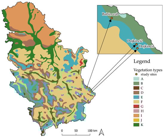
Figure 3.
Vegetation types in Serbia from the EPNV map: A, Alpine; subalpine and oro-Mediterranean vegetation; B, montane spruce and mixed spruce forests; C, montane pine forests; D, acidophilous oak and mixed oak-hornbeam forests; E, beech and mixed beech forests; F, thermophilous mixed bitter, pedunculate, or sessile oak forests; G, south-east Balkan sub-Mediterranean mixed oak forests; H, south-west Balkan sub Mediterranean mixed oak forests; I, Pannonian lowland mixed oak forests and steppes; J, Mediterranean mixed forests; K, hardwood alluvial forests, wet lowland forests, and swamps.
The percentage coverage of each class was calculated after land cover classified maps were obtained. Furthermore, classes from land cover classified maps that represent the possible natural elements of habitats which correspond to the vegetation types in the EPNV were chosen on each study site. The percentage coverage of classes that represent the natural elements of habitats was summarized, and the sum of the rest of the classes represents the percentage coverage of degraded habitat.
Several limitations of the EPNV map with respect to the UAV land cover classified maps were addressed, which are related to spatial resolution and mismatch in different approaches to defining vegetation types. Despite its limitations, it was necessary to use it as a starting point from which the current land cover can be determined.
2.6. Studied Hoverfly Material
Potential hoverfly species richness list was extracted from the results obtained by Miličić et al (2020) for certain vegetation types that correspond to the three study sites [57]. This list was composed based on the fact that each hoverfly species was assigned to any vegetation type in the EPNV, taking into consideration its known distribution across Europe and biological and ecological preferences of that species. Species typically found in three vegetation types were used: A, B, and E. The vegetation type E includes 355 hoverfly species, whereas the vegetation type A+B contains 166 hoverfly species (Table S13). Sum of species in the vegetation type A+B includes reduced number of species from the initial list from Miličić et al (2020), due to local specificity and a lack of certain landscape elements (further explained in the Discussion section).
During the thirty years of research on the three selected study sites, the list of recent hoverfly species richness was generated, based on the carefully collected and thoroughly examined material. Study sites were each surveyed by transect walks each year using a consistent census protocol [23]. Transect length was approximately 1–2 km, which was walked at a slow pace (15 m/min) along transects, and every hoverfly observed was recorded within a 3-m-wide area. Transects were conducted between 9.00 a.m. and 1.00 p.m. on sunny days with little or no wind. Hoverflies were either identified to species level in the field or, if specimens could not be identified on the wing, were caught with an entomological net and identified in the Laboratory for Biodiversity Research and Conservation, Department of Biology and Ecology, FSUNS, led by prof. dr. Ante Vujić. The database was previously used in some studies [26,32,57] for addressing different ecological questions. In this study, the subset of database containing hoverfly species richness in three sites was used. This list includes 44 hoverfly species in the study site Dojkinci1, 108 species in the Dojkinci2, and 38 species in the study site Babin zub (Table S14).
Comparison of the potential and recent richness of hoverfly species on each of the three study sites enables obtaining the insight into the overview of the hoverfly species richness and their connectedness with habitat degradation.
3. Results
3.1. Accuracies of the Classification Algorithms
The validity of the produced land cover maps was estimated using confusion matrices, the Kappa index, and the overall accuracy for all three tested classification algorithms: SVM, RF, and k-NN (Table 4). According to Table 4, the RF classifier achieved both the best overall accuracy and Kappa index when compared to other classifiers. Thus, only confusion matrices for the RF classifier are given in Figure 4. Detailed information, such as the precision, recall, and f-score per class for SVM, RF, and k-NN, is presented in Supplementary Materials.
Table 4.
Calculated overall accuracies (OA) and Kappa indices (k) for SVM, RF, and k-NN classifiers for all three study sites.
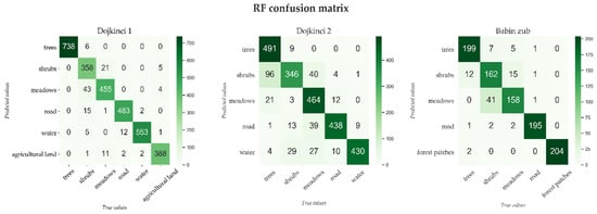
Figure 4.
Confusion matrices of RF classifier for Dojkinci1, Dojkinci2, and Babin zub.
3.2. Land Cover Classification Maps
The following classified land cover maps (Figure 5, Figure 6 and Figure 7) are presented for the best classification algorithm performances, which were developed with the RF classifier for all three study sites in all cases (Figure 4). The classification was performed using six land cover classes (trees, shrubs, meadows, road, water, and agricultural land) for the study site Dojkinci1; five land cover classes (trees, shrubs, meadows, road, and water) for the study site Dojkinci2; and five land cover classes (trees, shrubs, meadows, road, and forest patches) for the study site Babin zub.
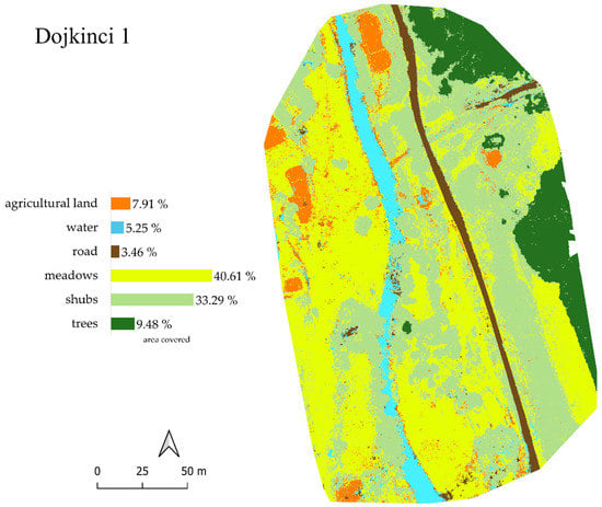
Figure 5.
Map of the land cover classification of the study site Dojkinci1 obtained by RF classification algorithm.
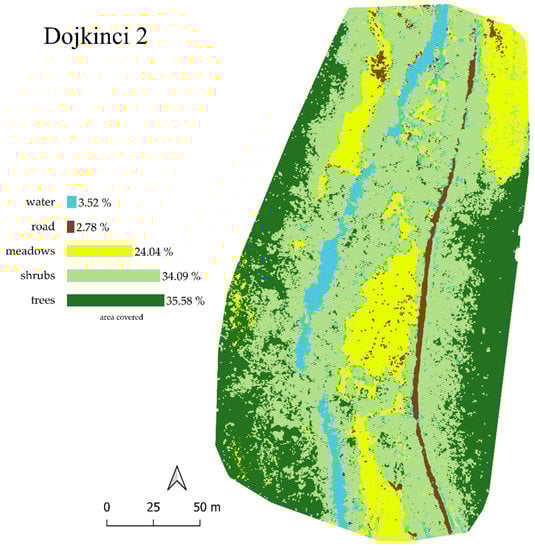
Figure 6.
Map of the land cover classification for the study site Dojkinci2 obtained by RF classification algorithm.
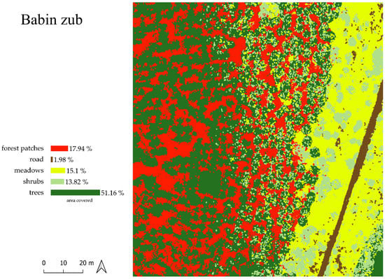
Figure 7.
Map of the land cover classification for the study site Babin zub obtained by RF classification algorithm.
For the study site Dojkinci1, the overall accuracy of the RF classification was 0.96, and the Kappa index was 0.95 (Table 4). The map of classified land cover with a percentage representation of each of the classes is given in Figure 5. The most dominant classes are meadows and shrubs, ranging between 35-40%. The trees class represents approximately 9%, the agricultural land represents 5.78%, the water amounts to 5.22%, whereas the road covers 3.74%. The shrub class presented a lower accuracy compared to the other classes. Several objects in the meadow class were incorrectly classified as agricultural land because of the similarities in spectral response and physiognomy of the plants in each of the classes.
In the study site Dojkinci1, the classes of trees and water belong to the natural elements of habitats, and constitute 14.56%. The rest of the classes (shrubs, meadows, road, and agricultural land) constitute 85.44%, which together represent the percentage coverage of habitat degradation.
According to the list of potential hoverfly richness (Table S13), the number of hoverfly species in this study site is estimated to be 355, whereas the number of registered hoverfly species (Table S14) is only 44 (Figure 8A), which amounts to 12.4% (Figure 8B). This number indicates a significant decline in species richness of 87.6% (Figure 8B). Apart from this, the percentage is close to the above-mentioned habitat degradation rate of 85.44% (Figure 8C).
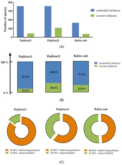
Figure 8.
(A) number of potential and recent hoverfly species in all three study sites; (B) calculated percentage of recent number of hoverfly species in relation to potential number of hoverfly species in conducted study sites; (C) ratio of habitat degradation and natural habitat (%).
In the study site Dojkinci2, the overall accuracy of the RF classification was 0.87, and the Kappa index was 0.84 (Table 4). The map of classified land cover with a percentage representation of each class for this study site is given in Figure 6. In this dataset, the class agricultural land disappears by moving away from the urban area deeper into the forest. When analyzing the distribution of classes, the highest percentage is attributed to trees with 35.58%, whereas shrubs cover 34.09%, meadows 24.04%, water 3.52%, and the road 2.78% of the total area.
In the study site Dojkinci2, only the classes of trees and water belong to the natural elements of habitats, and constitute 39.1%. The rest of the classes (shrubs, meadows, and road) constitute 60.9%, which together represent the percentage coverage of habitat degradation (Figure 8C).
According to the list of potential hoverfly richness, the number of hoverfly species in this study site is estimated to be 355, whereas the number of registered hoverfly species is 108 (Figure 8A), which amounts to 30.4% (Figure 8B). This percentage indicates a significant decline in species richness of 69.6% (Figure 8B).
In the study site Babin zub, the overall accuracy of the RF classification was 0.91, and the Kappa index was 0.89 (Table 4). The map of classified land cover with a percentage representation of each of the classes is given in Figure 7. This is a forest region, and accordingly, in orthomosaics, the largest share is attributed to trees with 51.16%, whereas forest patches have a share of 17.94%, meadows have 15.1 %, shrubs have 13.82%, and roads have less than 2%.
In the study site Babin zub, only the class of trees belongs to the natural elements of habitats, constituting 51.16%. The rest of the classes (forest patches, shrubs, meadows, and road) constitute 48.84%, which together represent the percentage coverage of habitat degradation (Figure 8C).
According to the list of potential hoverfly richness, the number of hoverfly species in this study site is estimated to be 166, whereas the number of registered hoverfly species is only 38 (Figure 8A), which amounts to 22.9% (Figure 8B). This percentage indicates a significant decline in species richness of 77.1% (Figure 8B).
The list of protected and strictly protected species of hoverflies in Serbia was used to determine which species are found in all three study sites. There is only one protected hoverfly species (Myolepta potens (Harris), 1780) in the study site Dojkinci1, and one protected (Cheilosia personata Loew, 1857) and one strictly protected (Merodon desuturinus Vujić, Šimić, and Radenković, 1995) in Dojkinci2. There are no protected nor strictly protected hoverfly species registered [87] in the study site Babin zub.
Time efficiency is a major factor, aside from the accuracy of the classifier. Classification time is the time required to predict the class labels for the given set of input data. The time duration for the training classifiers is presented in Table 5. Classifiers such as RF and k-NN are faster when compared to the SVM classifier. However, SVM requires more training time, and its performance is more sensitive to parameter adjustment in comparison to the other two classifiers [81,88].
Table 5.
Time duration for training vector classifiers.
4. Discussion
4.1. Data Acquisition in Complex Landscapes
This section aims to evaluate the potential of UAV technology in obtaining detailed classified land cover maps by taking into consideration various flight limitations and complexities of the terrain, especially in the study site Babin zub.
The results show that the landscapes, although geographically near to one another, easily pass from one class to another. The detection of such delicate changes in the ground cover from VHR images provided by UAVs is suitable. As small-scale changes cannot be detected at low resolutions (see Figure 3), it is important to address the possibility of obtaining high spatial and temporal resolution UAV data that are suitable for generating detailed land cover maps [89].
Depending on the angle of the slope, as well as the placement of the created UAV mission and the path planning in the position of the study site, the area covered by an UAV may be altered: it can be either increased or decreased. Uneven terrains, especially the mountain tops, can be obstacles to photogrammetry software. These errors and the noise caused by altitude differences during the image acquisition process significantly limit the overall image stitching capabilities of the photogrammetry software and appear as distortions in the final orthomosaic. The orthomosaic is generated based on the DSM. Therefore, errors and noise that are present in the densified point cloud will be reflected in the orthomosaic [90]. With this in mind, certain parts of the acquired UAV images must often be modified and sometimes even discarded. Nevertheless, they are carefully analyzed in order to make the most of the depth of field provided by the UAV. One of the possible solutions while collecting UAV images in complex terrains is to increase the overlap between images and to increase the number of the GCPs in order to enhance the orthorectification and overall quality of the orthomosaic [89,91]. The study site Babin zub, located on the top of the mountain, was demanding not only for UAV image acquisition but also for the performances of the photogrammetry software. It is clear that the center of the orthomosaic has a higher positional precision and accuracy than areas along the edges, simply because they consist of more images collected along the flight path [92]. Therefore, it is highly recommended that the central part of the orthomosaic should be chosen for further segmentation and classification procedures because it contains the least visual artifacts and noise, due to a lack of both key points in the marginal images and differences in terrain in complex landscape study sites. For Dojkinci1 and Dojkinci2, the whole orthomosaic was taken for the image-processing procedure.
4.2. Segmentation, Classifier’s Optimization, and Performances
The segmentation procedure is crucial and a prerequisite for accurate classification in OBIA. Segmentation enhancement can be carried out by adding a greater spectral range [93]. Furthermore, Husson et al. (2017) proved that classification accuracy can be significantly improved by adding a DSM layer in the automated classification of non-submerged aquatic vegetation [94]. Compared to the previously published research, where red, green, and NIR bands were available and obtained NDVI and DSM [38], in this research, the blue channel was replaced with NIR. Two flight missions were obtained with RGB and modified NDVI cameras and there were five spectral layers in total: red, green, blue, NDVI, and DSM (Figure 2). An appropriate range radius value during the image segmentation process is critical for a proper determination of classes. Optimizing the range radius value is crucial for breaking objects or polygons into parts that will be assigned to classes, and needs to be balanced between over and under segmentation extremes. If the segmented orthomosaic is not fragmented enough, in the sense that it does not consist of enough polygons, it will not be possible to separate and assign that part to the appropriate class [70]. There can be another issue with imbalanced data sets: if there are not enough objects (polygons) for marking the data, the classification procedure and accuracy will be inadequate [81].
From three machine learning algorithms representing different approaches—the simple search for similar samples and more complex ones that are performed on kernels and trees—we have selected the one that provided both the best results and a good time performance. When trained on default parameters, RF provided slightly better results than SVM and k-NN. Taking into consideration the training as well as the run-time of the whole image, RF was chosen as the most suitable. Small modifications of the RF classifier applied in all three study sites provided the best classification results. Further improvements in the land cover classification maps can be developed by adding/fixing training sets where needed; specifically, when a classifier does not distinguish between two classes e.g., in Dojkinci2 (Figure 6), where, next to the road, there were misclassifications of water with shrubs. Assigning these polygons after the first training will result in a slight improvement in the classification results [93].
The biggest challenge in all three study sites was to distinguish between trees and shrubs and between shrubs and meadows, as they tend to resemble each other in composition, color, shape, and texture. However, as already mentioned in the study sites section, the shrubby vegetation varied the most in species richness; therefore, marking the different species of shrubs proved to be challenging for classification algorithm capabilities and performances, especially in the Dojkinci1 and Dojkinci2 study sites (Figure 5 and Figure 6). Notably, there is a slight inconsistency in the data introduced by the presence of objects in the orthomosaics that do not belong to any of the classes, such as rocks, landslides, and bare ground. These small objects, mostly presented in the Dojkinci1 and Dojkinci2 study sites, are associated with some of the designated classes; however, they constitute a negligibly small portion in the entire orthomosaic (Figure 5 and Figure 6). When the time performance is considered, SVM, which is based on maximizing the margin between two different classes, took the longest time in training processing. However, it offered a good generalization with no prior knowledge of the data. Although the k-NN classifier performs the fastest, it yielded a less accurate classification compared to SVM and RF (Table 4 and Table 5) [88]. Finally, RF provided the best results in terms of the accuracy of land cover classification, whereas its time performance was satisfactory.
4.3. Potential and Recent Hoverfly Species Richness in Relation to Habitat Condition Assessment
In situ observations that were conducted over 30 years of field work registered negligible or no changes in the habitat condition and land coverage within all three study sites. Conversely, UAV-based land cover classified maps, compared with the map of the EPNV, show significant differences in the habitat properties.
Several studies show that the effectiveness of local biodiversity conservation management would change with landscape structure. Recently, Jovičić et al. (2017) showed that landscape structure and land use influence species compositions of two large phytophagous hoverflies genera (Merodon Meigen, 1803 and Cheilosia Meigen, 1822) differently in South-Eastern Europe [32]. Moreover, a study assessing the habitat quality in relation to decreased species richness of the same two genera in Serbia over a 25-year period [33] using CORINE land cover maps revealed that landscape structural changes, specifically in aggregation, isolation/connectivity, and landscape diversity, were significantly correlated with species richness loss. However, the UAV classified land cover map provides much greater precision and more details than CORINE (CLC), which greatly contribute to obtaining more accurate results and a more realistic picture of species richness in studied ecosystems. Furthermore, the differentiation between land cover classes is impossible with higher resolution layers, such as pan-European high-resolution layers, as they are merged in more generalized layers that connect/mix land cover classes, which are important to separate, as they are typical landscape elements that hoverflies inhabit. Although covering large areas, the downside of the mid-resolution of CLC or other layers is that they are unable to reveal the delicate distinction in land cover classes, such as meadows or shrubs, whereas water, roads, and small agricultural fields are not even presented. Moreover, a transition from one land cover class to another is less accurate at a lower resolution.
In selected study sites, habitat areas acquired with UAV maps were enough to cover the flying areas hoverflies are taking during their lifetime. Extensive life history strategies and a broad range of functional characteristics, specifically the degree of specialisation and mobility, make hoverflies suitable model organisms for analysis, where habitat condition, land cover, and land use are linked to the community functioning across several scales [36].
Observing the UAV classified land cover map of Dojkinci1 in relation to the EPNV, it is concluded that, from the aspect of habitat significance to the hoverfly’s richness, only trees, which would correspond to forest and water corresponding to the river, represent the native state of vegetation and habitat (Figure 5). The other classes (shrubs, meadows, road, and agricultural land) represent the percentage coverage of degradation of the natural vegetation types, which is 85.44% (Figure 5). By comparing the UAV map to the EPNV, it is evident that there is a high level of disturbance, because this study site would originally belong to the vegetation type of beech and mixed beech forests. This mainly refers to anthropogenic activity, such as the expansion of agricultural land, extensive deforestation, grazing, recreation, and tourism.
In the study site Dojkinci2, comparing the UAV land cover classified map with the EPNV shows that only trees and water belong to the elements of native vegetation and habitat, whereas shrubs, meadows, and a road represent the degree of habitat conversion and degradation due to human impact. Results from this investigation indicate that the percentage of habitat degradation amounts to 60.9%. Based on the EPNV, this study site belongs to the vegetation type of beech and mixed beech forests. However, due to changes in land use caused by inadequate forest management and tourism, the percentage of the native state of vegetation has decreased considerably (Figure 6). Results from this investigation show that, in Dojkinci1, the percentage of preserved natural vegetation is lower (14.56%) than in Dojkinci2 (39.1%) due to the difference in land use activities and intensity of anthropogenic pressures (Figure 8C).
In the UAV classified land cover map of the study site Babin zub, only the class of trees corresponds to both the natural vegetation type of alpine, subalpine, and oro-Mediterranean vegetation and to montane spruce and mixed spruce forest. All other classes (forest patches, road, meadow, and shrubs) represent the degraded habitat, encompassing 48.84% of the surface of the study site. The percentage of forest patches, at nearly 18% (Figure 7), is relatively high, which indicates intense (extensive) deforestation. Other negative impacts that contribute to habitat degradation are tourism, recreation, urbanization, and the construction of ski tracks.
Pollinator declines are most likely related to habitat destruction and degradation following agricultural intensification and urbanization [26]. Anthropogenic activities modify and disable the habitat’s capacity to support native species that have naturally existed in an area prior to the unmodified condition [1]. For hoverflies, activities such as deforestation, conversion to meadows and pastures, ploughing, and tourism have an impact on their biodiversity. The above-mentioned reduced percentage of the natural vegetation cover in all three study sites, caused mainly by the anthropogenic pressure, resulted in a reduced number of recent hoverfly species (Figure 8A). Moreover, selected study sites that represent the natural habitats of hoverfly species threaten to be ruined in the near future due to uncontrolled anthropogenic perturbations, to such an extent that they will be unable to support and maintain the recent richness of hoverflies. When analyzing two study sites that are geographically near, Dojkinci1 and Dojkinci2, a significant difference between the number of recent hoverfly species, as well as the percentage of habitat degradation, is observed. A higher percentage of degradation and a significantly lower number of recent species is noted in the study site Dojkinci1. This result is a consequence of more intense influences of anthropogenic activities in Dojkinci1 compared to the study site Dojkinci2 (Figure 6 and Figure 7).
It is a known fact that hoverflies are found near water in all types of habitats in high percentages (80–90%). In each of the vegetation types in the EPNV map, they are mostly in parts of the landscape such as streams, rivers, lakes, and wet and swampy habitats, and around peat bogs (peateries) that are usually allocated in coniferous communities [30,34]. There are several reasons why a hoverfly chooses these habitats: (1) the microclimate around and in them favors most adult hoverflies; (2) there is a greater diversity of plant species which favors plant-related species of hoverflies, as well as a greater choice of flowers on which adults feed on; and (3) these parts of the landscape are usually accompanied with a partly open space, which again favors the distribution of adults because of the sunny areas that they frequent [30]. The list of species (S13) that exist for these vegetation types are included in all elements of the landscape. The key difference between Dojkinci 1 and 2 and Babin zub is the absence of all of the mentioned types of habitats connected to water on Babin zub, whereas in Dojkinci, the whole area lies along the Dojkinačka river. The influence on the reduction in the species richness on Babin zub is twofold. One reason is the lack of aquatic habitats that support species diversity and survival [95], and the other is the initial habitat degradation that occurred in the past due to human impact. Analyzing the UAV classified land cover map of Babin zub, a large portion of coniferous forests is irretrievably lost (Figure 7). Another example of habitat degradation is forests being converted into pastures and meadows. Therefore, the decline in the number of recent species is attributed both to human influence and to the initially smaller number of species (potential richness) due to the absence of important landscape elements on Babin zub.
A list of protected (44) and strictly protected (33) species of hoverflies in Serbia is compiled [87]. From that list, one protected species was registered in the study site Dojkinci1, one protected and one strictly protected species in Dojkinci2, and none of the protected and strictly protected species were registered on Babin zub. This matches the percentage of habitat and species richness preservation (Figure 8).
This type of data can contribute to enhance management practices by providing targets for restoration and improving naturalness, ecosystem conservation, and biodiversity preservation.
4.4. Publicly Available Data
One of the challenges addressed in remote sensing literature is that readers outside of the field have a limited understanding of the discipline. Findings made by ecologists and biologists are not limited to only their fields and should instead be applied to real-world problems and used to benefit ecology from several different perspectives [16]. Sharing data publicly and offering the possibility to test datasets and learn from tutorials is a strong educational point of this research. This is a valuable ecological asset for conservation ecologists and researchers worldwide who have a basic knowledge in acquiring UAV remote sensing data and OBIA operations. Sharing data publicly, along with baseline methods, while demonstrating the challenging aspects of the data, allows for finding the best solution to a problem [96]. This level of knowledge in image segmentation and classification can provide a detailed and yet versatile new research method for future ecologically oriented research. As more ecologists and conservation biologists become proficient users of remote sensing technologies, the way they collect data and answer their research questions will be possible with more varied technologies [15].
5. Conclusions
This research shows how UAV-based technology could be employed to assess habitat degradation and their impact on hoverflies species biodiversity. From the experimental results and with regard to research objectives, the following is concluded:
- It is possible to obtain VHR UAV land cover classified maps in more heterogeneous study sites, but pinpointing limiting factors of data acquired in a complex area with a high slope of the terrain needs to be addressed;
- Proposed UAV-based land cover classification, along with both the potential vegetation types obtained from the EPNV map and biodiversity expert knowledge, can be applied in order to quantify habitat degradation in selected study areas;
- The initial results of linking the quantified habitat degradation with the biodiversity loss indicate the utility of the proposed framework;
- Comprehensive supplementary materials, including image processing steps for producing the land cover classified map in the form of a video recording guidance, along with raw data, ensure research reproducibility.
Our study focuses on land cover/use as one of the aspects of habitat condition. Other factors, such as the weather condition and vegetation state, which are important for understanding natural dynamics, could be examined with additional time series data obtained from both UAV and climate models. In this sense, the presented work is a starting point for further similar research topics and steps towards establishing methodology that can contribute to species habitat protection, which is essential for biodiversity conservation.
Supplementary Materials
The following are available online at https://www.mdpi.com/article/10.3390/rs13163272/s1. Table S1: Dojkinci1 different partitions of training and validation sets, Table S2: Dojkinci2 different partitions of training and validation sets, Table S3: Babin zub different partitions of training and validation sets, Table S4: Precision, recall, and f-score per class for SVM, RF, and k-NN classifiers (corresponding overall accuracy, Kappa index results presented in the manuscript) for Dojkinci1 study site., Table S5: Precision, recall, and f-score per class for SVM, RF, and k-NN classifiers (corresponding overall accuracy, Kappa index results presented in the manuscript) for Dojkinci2 study site, Table S6: Precision, recall, and f-score per class for SVM, RF, and k-NN classifiers (corresponding overall accuracy, Kappa index results presented in the manuscript) for Babin zub study site, Table S7: Precision, recall, and f-score per class for SVM, RF, and k-NN classifiers for the first repetition for Dojkinci1 study site, Table S8: Precision, recall, and f-score per class for SVM, RF, and k-NN classifiers for the first repetition for Dojkinci2 study site, Table S9: Precision, recall, and f-score per class for SVM, RF, and k-NN classifiers for the first repetition for Babin zub study site, Table S10: Precision, recall, and f-score per class for SVM, RF, and k-NN classifiers for the second repetition for Dojkinci1 study site, Table S11: Precision, recall, and f-score per class for SVM, RF, and k-NN classifiers for the second repetition for Dojkinci2 study site, Table S12: Precision, recall, and f-score per class for SVM, RF, and k-NN classifiers for the second repetition for Babin zub study site, Table S13: The list of potential richness of hoverfly species for the certain vegetation types, Table S14: The list of recent richness of hoverfly species in three designated study sites.
Author Contributions
Conceptualization, B.I., A.V. and J.V.; methodology, B.I., P.L. and J.V.; validation, B.I. and P.L. and S.B.; formal analysis, B.I. and M.R.; investigation, B.I., A.V; writing—original draft preparation, B.I. and J.V.; writing—review and editing, all of the authors; visualization, B.I. and M.R. All authors have read and agreed to the published version of the manuscript.
Funding
This research has received funding from the European Union’s Horizon 2020 research and innovation program under SGA-CSA. No. 739570 under FPA No. 664387 (ANTARES), through which the general research topic was identified as part of the ANTARES Joint Strategic Research Agenda, and No. 810775 (DRAGON), through which the specific theme was further conceptualized and investigated through the field work. The financial support of the Ministry of Education, Science and Technological Development of the Republic of Serbia is acknowledged (Grant No. 451-03-9/2021-14/200358) for authors B.I., P.L., S.B. and M.R.
Institutional Review Board Statement
Not applicable.
Informed Consent Statement
Not applicable.
Data Availability Statement
The raw data (Images) presented in this study are openly available in Zenodo at https://doi.org/10.5281/zenodo.4482248. Video tutorial (Video) of image-processing steps is given at https://doi.org/10.5281/zenodo.4482323.
Acknowledgments
Author B.I. would like to express great appreciation to Giandomenico De Luca for valuable technical support at the very beginning of data processing.
Conflicts of Interest
The authors declare no conflict of interest.
References
- Harwood, T.D.; Donohue, R.J.; Williams, K.J.; Ferrier, S.; McVicar, T.R.; Newell, G.; White, M. Habitat Condition Assessment System: A new way to assess the condition of natural habitats for terrestrial biodiversity across whole regions using remote sensing data. Methods Ecol. Evol. 2016, 7, 1050–1059. [Google Scholar] [CrossRef]
- Komisija. Eiropas Commission Note on Setting Conservation Objectives for Natura 2000 Sites; Final Version 23, 8; European Commission: Brussels, Belgium, 2012. [Google Scholar]
- Fischer, J.; Lindenmayer, D.B. Landscape modification and habitat fragmentation: A synthesis. Glob. Ecol. Biogeogr. 2007, 16, 265–280. [Google Scholar] [CrossRef]
- Fritz, A.; Li, L.; Storch, I.; Koch, B. UAV-derived habitat predictors contribute strongly to understanding avian species-habitat relationships on the Eastern Qinghai-Tibetan Plateau. Remote Sens. Ecol. Conserv. 2018, 4, 53–65. [Google Scholar] [CrossRef]
- Laliberte, A.S.; Herrick, J.E.; Rango, A.; Winters, C. Acquisition, Orthorectification, and Object-based Classification of Unmanned Aerial Vehicle (UAV) Imagery for Rangeland Monitoring. Photogramm. Eng. Remote Sens. 2010, 76, 661–672. [Google Scholar] [CrossRef]
- Shahbazi, M.; Theau, J.; Ménard, P. Recent applications of unmanned aerial imagery in natural resource management. GIScience Remote Sens. 2014, 51, 339–365. [Google Scholar] [CrossRef]
- Garcia-Ruiz, F.; Sankaran, S.; Maja, J.M.; Lee, W.S.; Rasmussen, J.; Ehsani, R. Comparison of two aerial imaging platforms for identification of Huanglongbing-infected citrus trees. Comput. Electron. Agric. 2013, 91, 106–115. [Google Scholar] [CrossRef]
- Moon, H.-G.; Lee, S.-M.; Cha, J.-G. Land cover classification using UAV imagery and object-based image analysis-focusing on the Maseo-Myeon, Seocheon-Gun, Chungcheongnam-Do. J. Korean Assoc. Geogr. Inf. Stud. 2017, 20, 1–14. [Google Scholar] [CrossRef]
- Tang, L.; Shao, G. Drone remote sensing for forestry research and practices. J. For. Res. 2015, 26, 791–797. [Google Scholar] [CrossRef]
- Pádua, L.; Vanko, J.; Hruška, J.; Adão, T.; Sousa, J.J.; Peres, E.; Morais, R. UAS, sensors, and data processing in agroforestry: A review towards practical applications. Int. J. Remote Sens. 2017, 38, 2349–2391. [Google Scholar] [CrossRef]
- Gómez, C.; White, J.C.; Wulder, M.A. Optical remotely sensed time series data for land cover classification: A review. ISPRS J. Photogramm. Remote Sens. 2016, 116, 55–72. [Google Scholar] [CrossRef]
- Vincent, J.B.; Werden, L.; Ditmer, M.A. Barriers to adding UAVs to the ecologist’s toolbox. Front. Ecol. Environ. 2015, 13, 74–75. [Google Scholar] [CrossRef]
- Koh, L.P.; Wich, S.A. Dawn of Drone Ecology: Low-Cost Autonomous Aerial Vehicles for Conservation. Trop. Conserv. Sci. 2012, 5, 121–132. [Google Scholar] [CrossRef]
- Ogden, L.E. Drone ecology. BioScience 2013, 63, 776. [Google Scholar] [CrossRef]
- Anderson, K.; Gaston, K.J. Lightweight unmanned aerial vehicles will revolutionize spatial ecology. Front. Ecol. Environ. 2013, 11, 138–146. [Google Scholar] [CrossRef]
- Horning, N.; Fleishman, E.; Ersts, P.J.; Fogarty, F.A.; Zillig, M.W. Mapping of land cover with open-source software and ultra-high-resolution imagery acquired with unmanned aerial vehicles. Remote Sens. Ecol. Conserv. 2020, 6, 487–497. [Google Scholar] [CrossRef]
- Ivosevic, B.; Han, Y.-G.; Cho, Y.; Kwon, O. The use of conservation drones in ecology and wildlife research. J. Ecol. Environ. 2015, 38, 113–118. [Google Scholar] [CrossRef]
- Nex, F.C.; Remondino, F. UAV for 3D mapping applications: A review. Appl. Geomat. 2013, 6, 1–15. [Google Scholar] [CrossRef]
- Shi, J.; Wang, J.; Xu, Y. Object-based change detection using georeferenced UAV images. ISPRS Int. Arch. Photogramm. Remote Sens. Spat. Inf. Sci. 2012, 38, 177–182. [Google Scholar] [CrossRef]
- European Environment Agency (EEA). The Pan-European Component. Available online: https://land.copernicus.eu/pan-european (accessed on 1 March 2021).
- Bohn, U.; Gollub, G.; Hettwer, C.; Neuhäuslová, Z.; Raus, T.; Schlüter, H.; Weber, H. Map of the Natural Vegetation of Europe. Scale 1: 2500000; Bundesamt für Naturschutz: Bonn, Germany, 2000. [Google Scholar]
- IPBES. Intergovernmental Science-Policy Platform on Biodiversity and Ecosystem Services; Brondizio, E.S., Settele, J., Díaz, S., Ngo, N.T., Eds.; IPBES Secretariat: Bonn, Germany, 2019. [Google Scholar]
- Ghazoul, J. Buzziness as usual? Questioning the global pollination crisis. Trends. Ecol. Evol. 2005, 20, 367–373. [Google Scholar] [CrossRef]
- Kluser, S.; Pascal, P. Global Pollinator Decline: A Literature Review; UNEP/GRID-Europe: Geneva, Switzerland, 2007; pp. 1–10. [Google Scholar]
- Potts, S.G.; Biesmeijer, J.C.; Kremen, C.; Neumann, P.; Schweiger, O.; Kunin, W.E. Global pollinator declines: Trends, impacts and drivers. Trends Ecol. Evol. 2010, 25, 345–353. [Google Scholar] [CrossRef]
- Radenkovic, S.; Schweiger, O.; Milic, D.; Harpke, A.; Vujić, A. Living on the edge: Forecasting the trends in abundance and distribution of the largest hoverfly genus (Diptera: Syrphidae) on the Balkan Peninsula under future climate change. Biol. Conserv. 2017, 212, 216–229. [Google Scholar] [CrossRef]
- Rhodes, C.J. Pollinator Decline—An Ecological Calamity in the Making? Sci. Prog. 2018, 101, 121–160. [Google Scholar] [CrossRef]
- Speight, M.C.D. Species Accounts of European Syrphidae. Syrph Net Database Eur. Syrphidae 2018, 103, 302–305. [Google Scholar]
- Rotheray, G.E.; Gilbert, F. The Natural History of Hoverflies; Forrest Text: Cardigan, UK, 2011; pp. 333–422. [Google Scholar]
- Van Veen, M.P. Hoverflies of Northwest Europe: Identification Keys to the Syrphidae; KNNV Publishing: Utrecht, The Netherlands, 2004; ISBN 978-90-5011-199-7. [Google Scholar]
- Kaloveloni, A.; Tscheulin, T.; Vujić, A.; Radenković, S.; Petanidou, T. Winners and losers of climate change for the genus Merodon (Diptera: Syrphidae) across the Balkan Peninsula. Ecol. Model. 2015, 313, 201–211. [Google Scholar] [CrossRef]
- Jovičić, S.; Burgio, G.; Diti, I.; Krašić, D.; Markov, Z.; Radenković, S.; Vujić, A. Influence of landscape structure and land use on Merodon and Cheilosia (Diptera: Syrphidae): Contrasting responses of two genera. J. Insect Conserv. 2017, 21, 53–64. [Google Scholar] [CrossRef]
- Popov, S.; Miličić, M.; Diti, I.; Marko, O.; Sommaggio, D.; Markov, Z.; Vujić, A. Phytophagous hoverflies (Diptera: Syrphidae) as indicators of changing landscapes. Community Ecol. 2017, 18, 287–294. [Google Scholar] [CrossRef]
- Naderloo, M.; Rad, S.P. Diversity of Hoverfly (Diptera: Syrphidae) Communities in Different Habitat Types in Zanjan Province, Iran. ISRN Zoöl. 2014, 2014, 1–5. [Google Scholar] [CrossRef]
- Vujić, A.; Radenković, S.; Nikolić, T.; Radišić, D.; Trifunov, S.; Andrić, A.; Markov, Z.; Jovičić, S.; Stojnić, S.M.; Janković, M.; et al. Prime Hoverfly (Insecta: Diptera: Syrphidae) Areas (PHA) as a conservation tool in Serbia. Biol. Conserv. 2016, 198, 22–32. [Google Scholar] [CrossRef]
- Schweiger, O.; Musche, M.; Bailey, D.; Billeter, R.; Diekötter, T.; Hendrickx, F.; Herzog, F.; Liira, J.; Maelfait, J.-P.; Speelmans, M.; et al. Functional richness of local hoverfly communities (Diptera, Syrphidae) in response to land use across temperate Europe. Oikos 2006, 116, 461–472. [Google Scholar] [CrossRef]
- Karr, A.F. Why data availability is such a hard problem. Stat. J. IAOS 2014, 30, 101–107. [Google Scholar] [CrossRef]
- De Luca, G.; Silva, J.M.N.; Cerasoli, S.; Araújo, J.; Campos, J.; Di Fazio, S.; Modica, G. Object-Based Land Cover Classification of Cork Oak Woodlands using UAV Imagery and Orfeo ToolBox. Remote Sens. 2019, 11, 1238. [Google Scholar] [CrossRef]
- Ahmed, O.S.; Shemrock, A.; Chabot, D.; Dillon, C.; Williams, G.; Wasson, R.; Franklin, S.E. Hierarchical land cover and vegetation classification using multispectral data acquired from an unmanned aerial vehicle. Int. J. Remote Sens. 2017, 38, 2037–2052. [Google Scholar] [CrossRef]
- Gini, R.; Passoni, D.; Pinto, L.; Sona, G. Use of Unmanned Aerial Systems for multispectral survey and tree classification: A test in a park area of northern Italy. Eur. J. Remote Sens. 2014, 47, 251–269. [Google Scholar] [CrossRef]
- Natesan, S.; Benari, G.; Armenakis, C.; Lee, R. Land cover classification using a UAV-borne spectrometer. ISPRS Int. Arch. Photogramm. Remote Sens. Spat. Inf. Sci. 2017, 42, 269–273. [Google Scholar] [CrossRef]
- Shin, J.S.; Lee, T.H.; Jung, P.M.; Kwon, H.S. A Study on Land Cover Map of UAV Imagery using an Object-based Classification Method. J. Korean Soc. Geospat. Inf. Syst. 2015, 23, 25–33. [Google Scholar] [CrossRef][Green Version]
- Kalantar, B.; Bin Mansor, S.; Sameen, M.; Pradhan, B.; Shafri, H.Z.M. Drone-based land-cover mapping using a fuzzy unordered rule induction algorithm integrated into object-based image analysis. Int. J. Remote Sens. 2017, 38, 2535–2556. [Google Scholar] [CrossRef]
- Devereux, B.; Amable, G.; Posada, C.C. An efficient image segmentation algorithm for landscape analysis. Int. J. Appl. Earth Obs. Geoinformation 2004, 6, 47–61. [Google Scholar] [CrossRef]
- Wang, L.; Sousa, W.P.; Gong, P. Integration of object-based and pixel-based classification for mapping mangroves with IKONOS imagery. Int. J. Remote Sens. 2004, 25, 5655–5668. [Google Scholar] [CrossRef]
- Weih, R.C.; Riggan, N.D. Object-based classification vs. pixel-based classification: Comparative importance of multi-resolution imagery. Int. Arch. Photogramm. Remote Sens. Spat. Inf. Sci. 2010, 38, 6. [Google Scholar]
- Blaschke, T. Object based image analysis for remote sensing. ISPRS J. Photogramm. Remote Sens. 2010, 65, 2–16. [Google Scholar] [CrossRef]
- Hay, G.J.; Castilla, G. Geographic object-based image analysis (GEOBIA): A new name for a new discipline. In Object-Based Image Analysis; Blaschke, T., Lang, S., Hay, G.J., Eds.; Lecture Notes in Geoinformation and Cartography; Springer: Berlin/Heidelberg, Germany, 2008; pp. 75–89. ISBN 978-3-540-77057-2. [Google Scholar]
- Addink, E.A.; Van Coillie, F.M.; De Jong, S.M. Introduction to the GEOBIA 2010 special issue: From pixels to geographic objects in remote sensing image analysis. Int. J. Appl. Earth Obs. Geoinf. 2012, 15, 1–6. [Google Scholar] [CrossRef]
- Al-Najjar, H.A.H.; Kalantar, B.; Pradhan, B.; Saeidi, V.; Halin, A.A.; Ueda, N.; Mansor, S. Land Cover Classification from fused DSM and UAV Images Using Convolutional Neural Networks. Remote Sens. 2019, 11, 1461. [Google Scholar] [CrossRef]
- Ventura, D.; Bonifazi, A.; Gravina, M.F.; Belluscio, A.; Ardizzone, G. Mapping and Classification of Ecologically Sensitive Marine Habitats Using Unmanned Aerial Vehicle (UAV) Imagery and Object-Based Image Analysis (OBIA). Remote Sens. 2018, 10, 1331. [Google Scholar] [CrossRef]
- Bohn, U.; Zazanashvili, N.; Nakhutsrishvili, G. The map of the natural vegetation of Europe and its application in the Caucasus ecoregion. Bull. Georgian Natl. Acad. Sci. 2007, 175, 11. [Google Scholar]
- FAO Forestry Paper 163 FAO (Food and Agriculture Organization of the United Nations). Global Forest Resources Assessment Main Report; FAO: Rome, Italy, 2010. [Google Scholar]
- Smith, G.; Harriet, G. European Forests and Protected Areas: Gap Analysis; UNEP World Conservation Monitoring Centre: Cambridge, UK, 2000. [Google Scholar]
- Bohn, U.; Gollub, G. The Use and Application of the Map of the Natural Vegetation of Europe with Particular Reference to Germany; Biology and Environment: Proceedings of the Royal Irish Academy; Royal Irish Academy: Dublin, Ireland, 2006. [Google Scholar]
- Marinova, E.; Thiebault, S. Anthracological analysis from Kovacevo, southwest Bulgaria: Woodland vegetation and its use during the earliest stages of the European Neolithic. Veg. Hist. Archaeobot. 2007, 17, 223–231. [Google Scholar] [CrossRef]
- Miličić, M.; Popov, S.; Vujić, A.; Ivošević, B.; Cardoso, P. Come to the dark side! The role of functional traits in shaping dark diversity patterns of south-eastern European hoverflies. Ecol. Èntomol. 2019, 45, 232–242. [Google Scholar] [CrossRef]
- Stumph, B.; Virto, M.H.; Medeiros, H.; Tabb, A.; Wolford, S.; Rice, K.; Leskey, T. Detecting Invasive Insects with Unmanned Aerial Vehicles. In Proceedings of the 2019 International Conference on Robotics and Automation (ICRA); IEEE: Montreal, QC, Canada, 20 May 2019; pp. 648–654. [Google Scholar]
- Ivošević, B.; Han, Y.-G.; Kwon, O. Monitoring butterflies with an unmanned aerial vehicle: Current possibilities and future potentials. J. Ecol. Environ. 2017, 41, 12. [Google Scholar] [CrossRef]
- Kim, H.G.; Park, J.-S.; Lee, D.-H. Potential of Unmanned Aerial Sampling for Monitoring Insect Populations in Rice Fields. Fla. Èntomol. 2018, 101, 330–334. [Google Scholar] [CrossRef]
- De Castro, A.I.; Jiménez-Brenes, F.M.; Torres-Sánchez, J.; Peña, J.M.; Borra-Serrano, I.; López-Granados, F. 3-D Characterization of Vineyards Using a Novel UAV Imagery-Based OBIA Procedure for Precision Viticulture Applications. Remote Sens. 2018, 10, 584. [Google Scholar] [CrossRef]
- De Castro, A.I.; Torres-Sánchez, J.; Peña, J.M.; Jiménez-Brenes, F.M.; Csillik, O.; López-Granados, F. An Automatic Random Forest-OBIA Algorithm for Early Weed Mapping between and within Crop Rows Using UAV Imagery. Remote Sens. 2018, 10, 285. [Google Scholar] [CrossRef]
- Huang, H.; Lan, Y.; Yang, A.; Zhang, Y.; Wen, S.; Deng, J. Deep learning versus Object-based Image Analysis (OBIA) in weed mapping of UAV imagery. Int. J. Remote Sens. 2020, 41, 3446–3479. [Google Scholar] [CrossRef]
- Yurtseven, H.; Akgul, M.; Coban, S.; Gülci, S. Determination and accuracy analysis of individual tree crown parameters using UAV based imagery and OBIA techniques. Measurement 2019, 145, 651–664. [Google Scholar] [CrossRef]
- Sibaruddin, H.I.; Shafri, H.Z.M.; Pradhan, B.; Haron, N.A. UAV-based approach to extract topographic and as-built information by utilising the OBIA technique. J. Geosci. Geomat. 2018, 6, 21. [Google Scholar]
- Papakonstantinou, A.; Stamati, C.; Topouzelis, K. Comparison of True-Color and Multispectral Unmanned Aerial Systems Imagery for Marine Habitat Mapping Using Object-Based Image Analysis. Remote Sens. 2020, 12, 554. [Google Scholar] [CrossRef]
- Ivanišević, B.; Savić, S.; Saboljević, M.; Niketić, M.; Zlatković, B.; Tomović, G.; Lakušić, D.; Ranđelović, V.; Ćetković, A.; Pavićević, D.; et al. “Biodiversity of the Stara Planina Mt. in Serbia”—Results of the Project “Trans-Boundary Cooperation through the Management of Shared Natural Resources”; The Regional Environmental Center for Central and Eastern Europe (REC): Belgrade, Serbia, 2007; ISBN 978-86-7550-050-6. [Google Scholar]
- Popović, M.; Đurić, M. Butterflies of Stara Planina (Lepidoptera: Papilionoidea); Srbijašume: Belgrade, Serbia, 2014. [Google Scholar]
- Grizonnet, M.; Michel, J.; Poughon, V.; Inglada, J.; Savinaud, M.; Cresson, R. Orfeo ToolBox: Open source processing of remote sensing images. Open Geospat. Data Softw. Stand. 2017, 2, 15. [Google Scholar] [CrossRef]
- Torres-Sánchez, J.; Lopez-Granados, F.; Peña-Barragan, J.M. An automatic object-based method for optimal thresholding in UAV images: Application for vegetation detection in herbaceous crops. Comput. Electron. Agric. 2015, 114, 43–52. [Google Scholar] [CrossRef]
- OTB Development Team. OTB CookBook Documentation; CNES: Pais, France, 2019; Available online: https://www.orfeo-toolbox.org/ (accessed on 15 January 2021).
- CNES OTB Development Team. Software Guide; CNES: Paris, France, 2018. [Google Scholar]
- Cresson, R. A Framework for Remote Sensing Images Processing Using Deep Learning Techniques. IEEE Geosci. Remote Sens. Lett. 2018, 16, 25–29. [Google Scholar] [CrossRef]
- Michel, J.; Youssefi, D.; Grizonnet, M. Stable Mean-Shift Algorithm and Its Application to the Segmentation of Arbitrarily Large Remote Sensing Images. IEEE Trans. Geosci. Remote Sens. 2014, 53, 952–964. [Google Scholar] [CrossRef]
- Kecman, V. Support Vector Machines–An introduction. In Support Vector Machines: Theory and Applications; Wang, L., Ed.; Studies in Fuzziness and Soft Computing; Springer: Berlin/Heidelberg, Germany, 2005; Volume 177, pp. 1–47. ISBN 978-3-540-24388-5. [Google Scholar]
- Mountrakis, G. Support vector machines in remote sensing: A review. ISPRS J. Photogramm. Remote Sens. 2011, 13. [Google Scholar] [CrossRef]
- Breiman, L. Random forests. Mach. Learn. 2001, 45, 5–32. [Google Scholar] [CrossRef]
- Pal, M. Random forest classifier for remote sensing classification. Int. J. Remote Sens. 2005, 26, 217–222. [Google Scholar] [CrossRef]
- Kramer, O. K-nearest neighbors. In Dimensionality Reduction with Unsupervised Nearest Neighbors; Intelligent Systems Reference Library; Springer: Berlin/Heidelberg, Germany, 2013; Volume 51, pp. 13–23. ISBN 978-3-642-38651-0. [Google Scholar]
- Peterson, L.E. K-nearest neighbor. Scolarpedia 2009, 4, 1883. [Google Scholar] [CrossRef]
- Noi, P.T.; Kappas, M. Comparison of Random Forest, k-Nearest Neighbor, and Support Vector Machine Classifiers for Land Cover Classification Using Sentinel-2 Imagery. Sensors 2017, 18, 18. [Google Scholar] [CrossRef]
- Tadele, H.; Mekuriaw, A.; Selassie, Y.G.; Tsegaye, L. Land Use/Land Cover Factor Values and Accuracy Assessment Using a GIS and Remote Sensing in the Case of the Quashay Watershed in Northwestern Ethiopia. J. Nat. Resour. Dev. 2017, 38–44. [Google Scholar] [CrossRef]
- Cohen, J. A Coefficient of Agreement for Nominal Scales. Educ. Psychol. Meas. 1960, 20, 37–46. [Google Scholar] [CrossRef]
- McHugh, M.L. Interrater reliability: The kappa statistic. Biochem. Med. 2012, 276–282. [Google Scholar] [CrossRef]
- De Mast, J. Agreement and Kappa-Type Indices. Am. Stat. 2007, 61, 148–153. [Google Scholar] [CrossRef][Green Version]
- Nichols, T.R.; Wisner, P.M.; Cripe, G.; Gulabchand, L. Putting the Kappa Statistic to Use. Qual. Assur. J. 2010, 13, 57–61. [Google Scholar] [CrossRef]
- Law on Nature Protection. Strictly Protected Wild Species of Plants, Animals and Fungi; Official Gazette of RS, no. 36/2009, 88/2010 and 91/2010; corr. and 14/2016; Official Gazette of the Republic of Serbia: Belgrade, Serbia, 2016. [Google Scholar]
- Soumya, A.; Kumar, G.H. Performance Analysis of Random Forests with SVM and KNN in Classification of Ancient Kannada Scripts. Int. J. Comput. Technol. 2014, 13, 4907–4921. [Google Scholar] [CrossRef]
- Siebring, J.; Valente, J.; Franceschini, M.H.D.; Kamp, J.; Kooistra, L. Object-Based Image Analysis Applied to Low Altitude Aerial Imagery for Potato Plant Trait Retrieval and Pathogen Detection. Sensors 2019, 19, 5477. [Google Scholar] [CrossRef]
- Distortions and Artifacts in the Orthomosaic. Available online: https://support.pix4d.com/hc/en-us/articles/202561099-Distortions-and-Artifacts-in-the-Orthomosaic (accessed on 1 March 2021).
- Using GCPs. Available online: https://support.pix4d.com/hc/en-us/articles/202558699-Using-GCPs (accessed on 15 March 2021).
- Hung, I.-K.; Unger, D.; Kulhavy, D.; Zhang, Y. Positional Precision Analysis of Orthomosaics Derived from Drone Captured Aerial Imagery. Drones 2019, 3, 46. [Google Scholar] [CrossRef]
- Momeni, R.; Aplin, P.; Boyd, D.S. Mapping Complex Urban Land Cover from Spaceborne Imagery: The Influence of Spatial Resolution, Spectral Band Set and Classification Approach. Remote Sens. 2016, 8, 88. [Google Scholar] [CrossRef]
- Husson, E.; Reese, H.; Ecke, F. Combining Spectral Data and a DSM from UAS-Images for Improved Classification of Non-Submerged Aquatic Vegetation. Remote Sens. 2017, 9, 247. [Google Scholar] [CrossRef]
- Vujić, A. Genus Cheilosia Meigen and Related Genera (Diptera: Syrphidae) on the Balkan Peninsula: Rod Cheilosia Meigen i Srodni Rodovi (Diptera: Syrphidae) Na Balkanskom Poluostrvu; Matica Srpska: Novi Sad, Serbia, 1996. [Google Scholar]
- Tsaftaris, S.A.; Scharr, H. Sharing the Right Data Right: A Symbiosis with Machine Learning. Trends Plant Sci. 2019, 24, 99–102. [Google Scholar] [CrossRef] [PubMed]


Publisher’s Note: MDPI stays neutral with regard to jurisdictional claims in published maps and institutional affiliations. |
© 2021 by the authors. Licensee MDPI, Basel, Switzerland. This article is an open access article distributed under the terms and conditions of the Creative Commons Attribution (CC BY) license (https://creativecommons.org/licenses/by/4.0/).