Abstract
The thermal Infrared Spectrometer (TIS) is the thermal infrared (TIR) sensor on-board the first Sustainable Development Goals (SDG-1) satellite. The TIS data can potentially be used to support improved monitoring of ground conditions with high-spatial resolutions, so accurate radiometric calibration is required. A meticulous radiometric calibration was conducted on the prototype of TIS to test its ability to convert a raw digital number (DN) to at-aperture radiance. The initial maximum radiometric error was 2.19 K at 300 K for Band 1(B1) and the minimum radiometric error was 0.25 K at 300 K rooted in Band 3 (B3). The R-Squared (R2) was over 0.99 for each band. The methodology was refined to divide the channel detectable temperature range into three sub-ranges and then the maximum radiometric errors were reduced to less than 1 K at 300 K for three bands. Subsequently, the Generalized Split-Window (SW) algorithm was preformed to estimate the ability of TIS on land surface temperature (LST) retrieval. In order to take advantage of its high-spatial resolution and make full use of TIR data, three-channel SW algorithm was also performed for intercomparison. Results showed that the SW algorithm can obtain LST with root-mean-square error (RMSE) less than 1K. Compared with two-channel algorithm with RMSE = 0.94 K, three-channel algorithm achieves better results in retrieving LST with RMSE = 0.82 K. For different land surface types, water samples achieved the minimum RMSE, and for different atmospheric column water vapor (CWV), dry atmospheres obtained better results. The sensitivity analysis of SW algorithm was considered along with noise-equivalent differential temperature (NEΔT), uncertainty of land surface emissivity (LSE) and input land surface temperature (). Generally, three-channel algorithm was more stable to LSE uncertainties, and the error changes were within 40%. But when NEΔT and uncertainties were included, the error percentage of three-channel SW method increases more, which means three-channel SW method is more sensitive to those two factors. All in all, the methodology and results used for radiometric calibration and LST retrieval in this study provide valuable guidance for the flight model of TIS and post-launch applications.
1. Introduction
Land surface temperature (LST) is a critical and reliable land surface feature parameter used to estimate land surface physical processes. Moreover, many other land surface parameters, such as evapotranspiration modeling [1] and soil moisture [2], rely on the prior knowledge of LST. Although the in situ temperature measurements could offer long-term coverage and highly accurate information, it is nearly impossible to used them for global monitoring. The thermal infrared (TIR) region is generally referred to a narrower range of 8~12 μm, which is an important atmospheric window for Earth science. Remotely sensed TIR data provide a simultaneous and large-scale view of land surfaces [3] and LST can be retrieving from TIR imagery. Therefore, TIR satellite imagery provides a quick method over different scales with a positive cost–benefit ratio. In recent decades, various thermal infrared remote sensing data sets have been acquired, as they can be widely applied for both Earth [4,5,6,7,8,9,10,11] and Mars [12,13,14,15,16,17].
The first Sustainable Development Goals (SDG-1) satellite is the first sustainable satellite developed by Chinese Academic of Sciences (CAS), and will be launched in 2021. It is intended to provide data support for the United Nations Sustainable Developed Goals. The satellite is intended to be used to provide scientific evidence for the refined depiction of human traces. Arctic and Antarctic observation is an expansion task for the SDG-1 satellite. The satellite needs to make a side swing to cover the entire 66.5°N/S to 90°N/S range. The SDG-1 satellite is equipped with three high-resolution optical payloads: Thermal Infrared Spectrometer (TIS), Glimmer Imager for Urbanization (GIU), and Multispectral Imager for Inshore (MII). The TIS is used for global thermal radiation detection and it has three TIR bands. The three TIR channels centered at 9.3 μm (8.0~10.5 μm, Band 1 (B1)), 10.8 μm (10.3~11.3 μm, Band 2 (B2)), and 11.8 μm (11.5~12.5 μm, Band 3 (B3)) with a spatial resolution of 30 m, which provides more spatial details than the TIR sensors currently in-orbit. Table 1 compares the thermal infrared band features of SDG-1 TIS and similar in-orbit sensors.

Table 1.
SDG-1 TIS and in-orbit sensor characteristics and thermal infrared band (8.0~12.0 μm) features.
The TIS data could be used to support improved monitoring of ground conditions, so an accurate radiometric calibration is firstly required. The accuracy of physical variables retrieved from remotely sensed data relies highly on the accuracy of radiometric calibration. The radiometric calibration process is to convert the digital number (DN) into the expected at-aperture radiance [18,19]. The DN is the raw signal from the detector that expressed as 12-bit numbers and the at-aperture radiance is the radiance enters the aperture that operates in units of . The preflight calibration ensures the instrument operates properly before being integrated into the launch vehicle, and provides a calibration method to be used after launch [18]. The preflight calibration of TIS was performed in a thermal-vacuum chamber against a laboratory blackbody and the calibration method that was used to determine the radiometric calibration of TIS was described in this paper.
Retrieving LST from TIR imagery is challenging as the radiance emitted from the surface in the infrared region is a function of temperature and emissivity. For a N band sensor, there will always be N+1 unknowns, corresponding to N emissivities at each band and an unknown temperature. Under specific assumptions, LST can be successfully retrieved from satellite measurements. Consequently, many algorithms have been developed to retrieve LST which can be generally classified into four categories [20,21]: the single-channel [22,23,24], day/night [25,26,27,28], split window (SW) [29,30,31,32,33] and temperature-emissivity separation (TES) methods [34,35]. Among these methods, SW is widely used because it can accurately remove the atmospheric effects by combining measurements from two adjacent channels at 11 and 12 μm. SW has been used in various satellite data to estimate LST, such as Advanced Very High Resolution Radiometer (AVHRR) [36], Moderate Resolution Imaging Spectroradiometer (MODIS) [29], Chinese Geostationary FengYun Meteorological Satellite (FY-2C) [37] and Chinese Gaofen-5 (GF-5) satellite data [31]. Herein, the Generalized Split-Window algorithm [28,29] was selected to firstly evaluate the ability of TIS on LST retrieval. As TIS sensor has three thermal infrared channels, three-channel SW algorithm was also adapted to estimate LST from TIS data.
This paper is organized as follows: Section 2 presents the theoretical basis for preflight radiometric calibration and the SW algorithm. A simulation data set was established for LST retrieval. Section 3 gives the results of radiometric calibration and LST retrieval. Improvement of radiometric calibration method was also performed. The LSTs retrieved by two SW methods were also compared. In addition, the effect of atmospheric column water vapor (CWV) was analyzed. The sensitivity analysis for SW algorithm is described in Section 4. The conclusions are drawn in Section 5.
2. Methods
2.1. Laboratory Radiometric Response Characteristic
The prototype of TIS was placed in a thermal-vacuum chamber that simulates the environment on-orbit, and then characterizes its radiometric response. The relationship between DN and at-aperture radiance was found by a three-step process [38]. The instrument background was removed first. Next, the expected at-aperture radiance was calculated with the emissivity and temperature of the blackbody and the channel spectral response (Equations (1) and (2)). Finally, linear regression was performed to obtain the radiometric calibration coefficients (Equation (3)).
where is the Planck radiance at the given blackbody temperature, ,,, is the spectral radiance of each channel, is the spectral response of each band, and is the emissivity of the blackbody.
where is the digital number after the background removal, and are the radiometric calibration coefficients of offset and gain, respectively.
2.2. Thermal Radiative Transfer Equation
Based on the radiative transfer theory and assuming a cloud-free atmosphere under thermodynamic equilibrium, the top of atmosphere (TOA) radiance received at each TIR channel can be written as Equation (4):
where represents SDG-1 TIR channel , is the top of atmosphere (TOA) radiance received by TIR channel . is the channel emissivity, is the channel blackbody radiance at LST (in K) calculated by the Planck function, and represents the surface emission radiance. is the upward channel-effective transmittance of the atmosphere in the channel and represents the surface emission attenuated by the atmosphere. is the channel upwelling radiance, and is the downward atmospheric thermal radiance reflected by the surface, represents the downward atmospheric thermal radiance reflected by surface and reaches the sensor. is the channel upwelling radiance. TOA radiance at each band can be converted to brightness temperature, and then, SW algorithm can be performed to retrieval LST.
2.3. Simulation Data Set
By using the moderate-spectral-resolution atmospheric transmittance model (MODTRAN) [39], the brightness temperatures of the three TIR channels of SDG-1 can be simulated with known atmosphere parameters, land surface emissivity (LSE), land surface temperature (LST), and channel response functions (CRF). The LST retrieval coefficients were subsequently regressed with the multiple linear regression method.
A total of 742 Thermodynamic Initial Guess Retrieval (TIGR) mid-latitude atmospheric profiles with column water vapor (CWV) ranging from 0.2 to 4.7 g/cm2 were selected to represent the most of the world atmospheric situations. The relationship between bottom layer temperature and water vapor content is plotted in Figure 1. Then, the atmosphere parameters (atmospheric transmittance, upwelling radiance and downwelling radiance) were simulated by MODTRAN from atmospheric profiles.
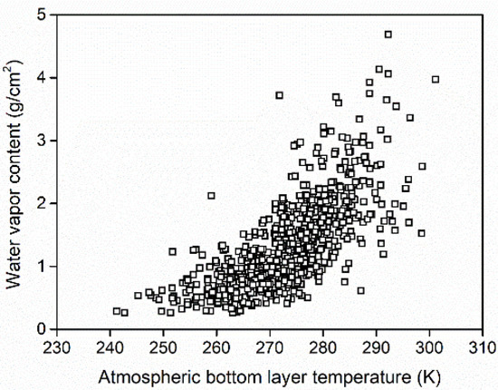
Figure 1.
Scatter plot of the bottom layer temperature and water vaper content of the 742 atmosphere profiles.
Emissivity spectra were selected from the ECOSTRESS spectral library, Version 1.0 (https://speclib.jpl.nasa.gov/, accessed on 22 March 2018) covering different types of land surfaces. The total of 68 LSEs consisted of 21 soils, 24 rocks and minerals, 12 vegetation, 5 water samples and 6 man-made targets. Channel effective emissivity (ε) was calculated by the following Equation (5):
where ε(λ) is the emissivity spectra, R(λ) is the CRF of the SDG-1 TIS sensor. The land surface temperature () was determined according to the bottom later temperature of the atmospheric profiles () at 7 levels that varied from − 10 K to + 20 K with an interval of 5 K.
With the parameters described above, the simulation data set was created and contained 353,192 different cases (742 atmospheric profiles 68 LSEs 7 LSTs).
2.4. Split Window (SW) Algorithm
As the TIS sensor onboard SDG-1 satellite has two adjacent thermal infrared channels centered at about 11 and 12 μm, the Generalized Split-Window algorithm proposed by Wan and Dozier [29] was used to retrieve LST from SDG-1 data and the LST could be expressed as:
with , .
In addition, and are the TOA brightness temperatures in B2 (~11 μm) and B3 (~12 μm). and are the land surface emissivity in B2 and B3, respectively. are the algorithm coefficients. The method was refined by adding a quadratic term of the brightness temperature difference of the two channels that improve LST accuracy under hot humid atmospheric condition [25], and the equation can be written as follows:
where denote the algorithm coefficients.
Considering that SDG-1 has three TIR channels and make full use of the data, a three-channel SW algorithm [40] was also selected to verify the performance of the proposed algorithm. This algorithm can be expressed as:
where are the algorithm coefficients.
The coefficients of two- and three-channel SW algorithm were obtained by the multiple regression method. The LSTs, emissivity and TOA brightness temperature were all from simulation datasets.
3. Results
3.1. Radiometric Calibration Results
The temperature of the blackbody was set as 230 K, 240 K 250 K, 270 K, 290 K, 300 K, 310 K, 320 K and 330 K, which span the required sensitivity range of the prototype of TIS. The relationship between the given temperatures and the measured temperatures are illustrated as Figure 2. At 230 K and 310 K points, the difference was relatively high as 1.97 K and 2.57 K, respectively, which means the linear response of the blackbody needs some improvements. However, for the most given temperatures, the difference was within 0.50 K, and the standard deviation was within 0.20 K. Therefore, the blackbody was stable to provide reliable experimental results.
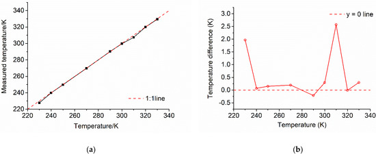
Figure 2.
(a) The relationship between the given temperature (x-axis) and the measured temperature (y-axis). Red dashed line represents 1:1 line that measured temperature and given temperature are same. (b) Temperature differences between the given temperature and the measured temperature at different given temperature points. Red dashed line represents y = 0 line that temperature difference is 0 K.
The channel response functions of the prototype of TIS are shown in Figure 3. B1 is a wide band, while B2 and B3 are narrower.
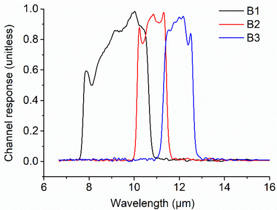
Figure 3.
The channel response functions of the prototype of Thermal Infrared Spectrometer (TIS). B1: Band 1; B2; Band 2; B3: Band 3.
The expected radiance was calculated by computing the Planck blackbody function at the given temperature. The emissivity of the blackbody is taken as 0.985 for all wavelengths. The temperature-radiance look-up table (LUT) for each band was established. The relationship between DN (background subtracted) and expected radiance for the range recorded temperatures is shown in Figure 4.
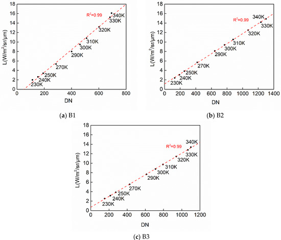
Figure 4.
Calculated spectral radiance for nine given temperatures as a function of the DN (background subtracted). (a) The DN (x-axis) versus spectral radiance (y-axis) for B1. (b) The DN (x-axis) versus spectral radiance (y-axis) for B2. (c) The DN (x-axis) versus spectral radiance (y-axis) for B3. Red-dashed lines are linear regression results. R2 is R-Squared. Red dashed lines are the linear fitting results of each band.
As shown in Figure 4, the fitting lines distribute closely to points at measured temperatures, and R2 is over 0.99 for each band. Consequently, there is a good linear correlation between calculated radiance and DN. The radiance differences between the expected at-aperture radiance and linear-regressed radiance (the residuals of the fitting) are illustrated in Figure 5. The radiance differences are distributed around zero. The B1 is the worst fitting case, while B3 achieves the best fitting results among all three bands. The maximum radiometric error was 0.37 , corresponding to 2.19 K at 300 K for B1 and the minimum radiometric error was 0.03 , corresponding to 0.25 K at 300 K for B3.
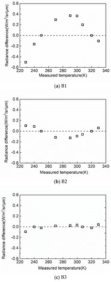
Figure 5.
The residuals of the fitting results for (a) B1, (b) B2 and (c) B3 at given temperature points.
In addition, the radiometric resolution at each given temperature was calculated and the results were plotted in Figure 6. The radiometric resolution was defined as the temperature change corresponding to 1 DN variation. B1 has the highest radiometric resolution because it needs a higher temperature for 1 DN change. The radiometric resolution is quite similar for B2 and B3. In general, the radiometric resolution decrease as the given temperature increases, except for the 310 K point.
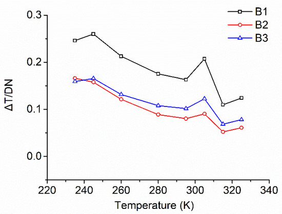
Figure 6.
Radiometric resolution for bands B1, B2 and B3 at given temperatures.
3.2. Improvement of the Radiometric Calibration
As shown in Figure 5, the fitting residuals of B1(Figure 5a) and B2(Figure 5b) have one turning point at 290 K, and residuals are close to zero at 250 K and 320 K. Hence, the whole temperature range was divided into three subranges and radiometric calibration was performed in three subranges for three bands. The three subranges are (230, 270) K, (270, 310) K, and (310, 330) K for low, middle, and high temperatures, respectively. These feature points are contained in the three subranges, which can get better fitting results.
The results are shown in Figure 7. The accuracy has been greatly improved as the radiance difference is within (−0.1, 0.1) in most cases and the radiometric error is less than 1 K at 300 K for three bands.
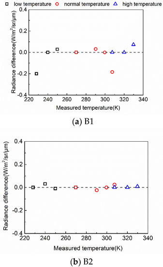
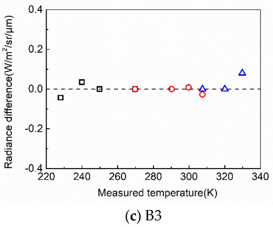
Figure 7.
Regression residuals in three subranges for three bands: (a) B1, (b) B2 and (c) B3.
In conclusion, performing a calibration process in different sub-temperature ranges is an effective way to improve the radiometric calibration accuracy.
3.3. LSTs Retrieval Results
The simulation data set described in Section 2.3 was applied to obtain the SW algorithm coefficients and the results are summarized in Table 2. The SW algorithm was developed with known LSEs. Therefore, the retrieval results varied for different land surface types. The overall root-mean-square error (RMSE) of LST estimation of two-channel SW algorithm was 0.94 K and R2 was 0.99. The RMSE of LST varied from 0.75 K to 1.08 K for different land surfaces. The SW algorithm performed best for water samples, and was less accurate for soil samples. The particle size, moisture, chemical composition, organic matters, etc. are different in different soil samples which lead to more variations in emissivity spectra. Hence, the temperature simulated by MODTRAN varied and lead to higher RMSEs. ΔLST (the difference between the actual LST and predicted LST) histograms of different land surface types are presented in Figure 8 for both two-channel and three-channel algorithm. The figures illustrate that most of the LST differences fell in the range of (−1, 1) K, and the mean value of ΔLST is very close to 0 K.
Table 2.
The overall root-mean-square error (RMSE) of two- and three-channel split window (SW) algorithm for different land surface types.
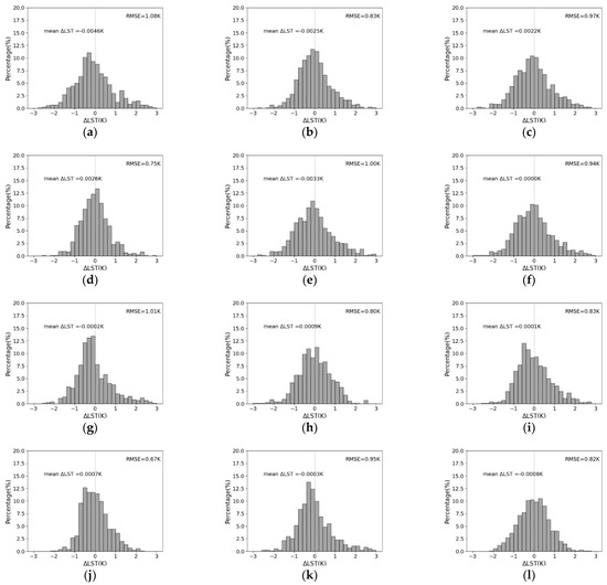
Figure 8.
Histogram of the difference between the actual LST and predicted LST (ΔLST) for different land surface types. Two-channel SW algorithm: (a) Soil, (b) Rock and minerals, (c) Vegetation, (d) Water, (e) Man-made, (f) All types. Three-channel SW algorithm: (g) Soil, (h) Rock and minerals, (i) Vegetation, (j) Water, (k) Man-made, (l) All types. Dash lines represent the mean value of ΔLST.
The RMSEs for three-channel SW algorithm is less than that for the two-channel SW algorithm. The smallest RMSE is 0.67 K for water samples with the highest R2 = 0.99, and the largest RMSE is 1.01 K for soils. The overall RMSE is 0.82 K. From this point of view, the three-channel algorithm performs better as the RMSEs are lower.
Atmospheric CWV is a factor that influence the LST retrieval results. In order to see the effects of the CWV on the retrieval of LST, all 742 TIGR profiles was divided into three subranges according to CWV with an overlap of 0.5 g/cm2 [31]. The three subranges are (0.0, 2.0), (1.5, 3), and (2.5, 5) g/cm2, represent low, middle and high CWV, respectively. Herein, 628 profiles for low CWV, 229 profiles for middle CWV and 53 profiles for high CWV. The SW algorithm was also performed based on different CWV subranges. The results in Table 3 presented that LST RMSE increased from 0.71 K to 1.13 K for the two-channel algorithm, and from 0.69 K to 0.94 K for the three-channel algorithm as CWV increased. The best fitting result occurred in dry atmospheric conditions, which has the lowest RMSE. With the increasing CWV, the RMSE of the two-channel algorithm increased by 0.42 K, which is higher than the 0.25 K of the three-channel algorithm.
Table 3.
RMSEs of two- and three- channel SW algorithm for different column water vapor.
4. Discussion
4.1. Sensitivity Analysis of TIS for LST Retrieval
A better LST algorithm must have the following features: (1) it retrieves LST more accurately; (2) it is less sensitivity to uncertainties, such as surface parameters, atmospheric properties, the instrument responses, etc. [29,31,37]. Therefore, noise equivalent differential temperature (NEΔT) of the sensor, the different input LSTs and uncertainties in LSEs were taken into account in this investigation.
4.1.1. Sensitivity to Instrument Noise
The NEΔT influences the accuracy of LST retrieval. The TIS onboard SDG-1 satellite was designed with NEΔT= 0.2 K. In order to estimate the effect of NEΔT on LST retrieval, a Gaussian noise was added to TOA brightness temperatures in Equations (7) and (8). The standard deviation of the noise was equal to designed NEΔT of the TIS sensor and then LST was estimated with noised TOA brightness temperatures. Table 4 shows the change of RMSE caused by NEΔT of the instrument. The NEΔT contributed noteworthy error to water samples which about 0.27 K (37.33% error increase) and 0.15 K (22.39% error increase) for two-channel and three-channel SW algorithms, respectively. LST RMSE increased by 0.10 K and 0.14 K after the noise was added to brightness temperature for two- and three-channel algorithm, respectively. That is to say, the two-channel algorithm is less sensitivity to NEΔT than the three-channel algorithm in most cases.
Table 4.
LST errors caused by NEΔT for different land surface types.
The error caused by NEΔT in different CWV subranges was also compared and the results are shown in Table 5. The error increase percentage changes less under high CWV conditions. The RMSE increased with increasing CWV, for the same RMSE variation, it contributes to a lower percentage change in large RMSE. As a result, the error increase percentage achieved the lowest value in high CWV subranges. For two SW methods, three-channel SW algorithm has lower RMSE, but in high CWV and all CWV conditions, two-channel SW algorithm performs more stable with less error increase percentage.
Table 5.
LST errors caused by NEΔT for different column water vapor.
4.1.2. Sensitivity to LSEs
LSE is a key factor that is related to LST retrieval. According to Equation (7), terms and are influenced by uncertainties in LSE. In Equation (8), term is influenced by uncertainties in LSE. In addition, the radiative transfer process is also different based on different LSE. Herein, about (−2%, 2%) error with intervals of 1% was added to investigate the retrieval accuracy when errors were contained in LSEs. Using the two SW retrieval methods, the obtained LST RMSE are shown in Table 6. Results show that the RMSE increased when emissivity errors were introduced. The error has a larger influence on LST results when emissivity is overestimated. It can also be seen from Table 6 and Figure 9, that the RMSE of the three-channel algorithm have less RMSE than the two-channel algorithm, which means that more bands in LST retrieval could decrease the sensitivity to emissivity errors.
Table 6.
LST RMSE caused by emissivity uncertainty.
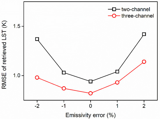
Figure 9.
The RMSE of retrieved LST for different SW algorithm as a function of emissivity errors.
4.1.3. Sensitivity to
In the simulation dataset, the surface temperatures were designed in seven levels based on the bottom atmospheric temperature () of each atmospheric profile. Therefore, the multiple regression was performed separately for different to estimate how influenced the LST retrieval results. The RMSE of the LST retrieval based on different values showed that (in Table 7 and Figure 10), with an increasing , the RMSE decreased. When the input is 15 K to 20 K higher than , the RMSE reaches the minimum value. This result indicates that the real land surface temperature is about 15 K to 20 K higher than the bottom layer atmospheric temperature. In addition, the overall RMSE of the three-channel algorithm is lower than RMSE of the two-channel algorithm in different conditions, while ΔRMSE is higher for the three-channel algorithm. The three-channel algorithm is less stable with variation.
Table 7.
LST RMSE caused by estimation.
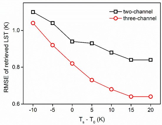
Figure 10.
The RMSE of retrieved LST for different SW algorithm as a function of estimated difference.
4.2. Comparision with Other TIR Sensors
MODIS provides Earth’s surface data for over 20 years and it is still in operation. The thermal infrared Band 29 (9.73 μm), Band 31 (11.03 μm) and Band32 (12.02 μm) are suitable for retrieval surface temperature. It provides LST products in long time series with a high-time resolution and it serves as a keystone for the satellites launched afterwards. The Generalized Split-Window algorithm was first proposed for retrieving LST from MODIS data [29]. Different MODIS LST products have been produced based on different algorithms, and the accuracy is generally better than 1 K after ground validation [41]. Although MODIS provides LST with high accuracy, the spatial resolution is only 1 km. Furthermore, the instrument’s performance over its entire orbital lifetime varies [42]. New TIR satellite sensors with high-spatial resolution for thermal infrared sensors are still needed to provide more detailed information on land surface. The pre-flight error of simulated LST from SDG-1 data is in the (−1,1) K range in most cases which is a little bit higher than MODIS LST products. However, 30 m spatial resolution is a big advantage when compared to MODIS 1 km spatial resolution.
Landsat 8 is the most recent satellite of Landsat Data Continuity Mission and the TIRS sensor has a relatively high spatial resolution. The new TIRS has two TIR bands and SW algorithm can be applied for LST retrieval [43]. The pre-flight radiometric calibration showed that when the fitting method is linear, the response of TIRS has a 0.4% error in the worst case [38], while it reaches over 0.7% for TIS. After the improvement of radiometric method, the error decreases to a low level which indicates the effective of the method. RMSE of LST estimated from TIRS using SW algorithm is 1.025 K for all samples [44] and it is comparable with simulated LST results of TIS. Due to the known instability in the system calibration of Band 11 (12.0 μm) [45,46], LST retrieved from Band 11 has more uncertainty than from Band 10 (10.9 μm) [43,44]. The stray light and striping artifacts made the calibration more challenging [38,45] and a stable and accuracy sensor is expected.
Recently, the Thermal Infrared Sensor-2 (TIRS-2) that will onboard Landsat 9 has finished its prelaunch testing [47]. TIRS-2 sensor has two TIR bands at 10.8 μm and 12.0 μm and the spatial resolution is 100 m (resampled to 30 m). The radiometric uncertainties for two channels are 0.5 K and 0.4 K [47] which are comparable with radiometric calibration results of prototype TIS sensor. The ability of TIRS-2 on LST retrieval has not been published yet. The two sensors will be further compared in a following work.
GF-5, the fifth satellite in the national high-resolution Earth observation project of China, has a four-channel TIR sensor with a spatial resolution of 40 m [48]. The four bands are centered at 8.20, 8.63, 10.80, and 11.95 μm, respectively. RMSE of LST retrieval from simulation data set for all surface types is 0.87 K using two-channel SW algorithm and 0.99 K for three-channel SW algorithm [31]. The error increase percentage is higher than SDG-1 TIS sensor when some uncertainties introduced in most cases. It indicates that TIS performs more stable on LST retrieval.
TIS onboard SDG-1 is a high-spatial-resolution TIR sensor. The 30 m spatial resolution will provide more detailed information on land surfaces, which is important for urban areas. As SDG-1 is not be launched, ground validation of retrieved LST from TIS image cannot be performed. The assessment of TIS on LST retrieval was mainly based on theoretical simulation results. Two selected SW algorithms reveal the potential of TIS on LST retrieval with high accuracy. The validate with field measurements in different regions will be updated after SDG-1 launches.
5. Conclusions
To ensure the scientific objectives of the SDG-1 mission, the TIS instrument needed to be accurately calibrated. A series of experiments were performed preflight on the prototype of TIS and a method was developed to convert the raw digital numbers from the detector into an at-aperture radiance. Background subtraction was first performed followed by the conversion to radiance, and finally, linear regression was performed to obtain the calibration coefficients. The whole tested temperature range was divided into three sub-ranges and regressed separately to improve the calibration accuracy, especially for B1. The radiometric calibration errors were less than 1 K for three bands.
SDG-1 will provide observations in three TIR channels at a fine spatial resolution of 30 m. To make full use of the TIR data, the Generalized Split-Window algorithm and a three-channel SW algorithm were used to estimate LST from SDG-1 data and the sensitivity of each algorithm was analyzed. The regression coefficients were obtained from simulation data based on MODTRAN model. The results showed that three-channel method performed better than two-channel method with RMSE lower than 1 K. For different land surface types, the minimum RMSE of LST retrieval was obtained for water samples and the maximum was acquired for soil samples as the spectra of soil samples have more variations than the water spectra. The algorithms were also performed in different CWV subranges and the RMSE of LST retrieval increased with the increase of CWV. A sensitive analysis was conducted with considerations involving NEΔT, uncertainty of LSE, and input land surface temperature, . Both SW algorithms used in this study have its advantages. The Generalized Split-Window algorithm is less sensitive to uncertainties in NEΔT and while the three-channel algorithm refined the retrieval results with less RMSEs. Different methods could be adapted for different purposes to retrieval LST. All in all, TIS channels were eligible to retrieve accurate LSTs using two- or three-channel SW algorithm.
The radiometric calibration and LST retrieval method conducted in this study provide a possible post-launch state which might be easier to control and modified after launch. Also, the TIS sensor has the potential to provide LST results with high spatial resolution. Finally, the results in this study provide guidance to develop a high-precision flight model of TIS instrument that will be equipped on the SDG-1 satellite to fulfil its scientific mission.
Author Contributions
Conceptualization, W.L. and J.L.; methodology, W.L., J.L. and Y.Z.; validation, Y.Z. and L.Z.; formal analysis, J.L.; resources, J.L.; writing—original draft preparation, W.L.; writing—review and editing, W.L., J.L., Y.Z., L.Z. and Q.C.; visualization, W.L.; supervision, J.L. and Q.C.; funding acquisition, J.L. All authors have read and agreed to the published version of the manuscript.
Funding
This research was funded by Strategic Priority Research Program of Chinese Academy of Sciences, grant number XDA19010403 and National Key Research and Development Program of China, grant number 2019YFE0126600.
Institutional Review Board Statement
Not applicable.
Informed Consent Statement
Not applicable.
Data Availability Statement
Not applicable.
Acknowledgments
The authors would like to thank Fansheng Chen and Zhuoyue Hu at Shanghai Institute of Technical Physics, Chinese Academy of Science, for providing the prototype of TIS with its laboratory results. This study was also funded by China Scholarship Council (CSC).
Conflicts of Interest
The authors declare no conflict of interest.
References
- Li, Z.-L.; Tang, R.; Wan, Z.; Bi, Y.; Zhou, C.; Tang, B.; Yan, G.; Zhang, X. A Review of Current Methodologies for Regional Evapotranspiration Estimation from Remotely Sensed Data. Sensors 2009, 9, 3801–3853. [Google Scholar] [CrossRef] [Green Version]
- Van Doninck, J.; Peters, J.; De Baets, B.; De Clercq, E.M.; Ducheyne, E.; Verhoest, N.E.C. The potential of multitemporal Aqua and Terra MODIS apparent thermal inertia as a soil moisture indicator. Int. J. Appl. Earth Obs. Geoinf. 2011, 13, 934–941. [Google Scholar] [CrossRef]
- Weng, Q. Thermal infrared remote sensing for urban climate and environmental studies: Methods, applications, and trends. ISPRS J. Photogramm. Remote Sens. 2009, 64, 335–344. [Google Scholar] [CrossRef]
- Ninomiya, Y.; Fu, B. Thermal infrared multispectral remote sensing of lithology and mineralogy based on spectral properties of materials. Ore Geol. Rev. 2019, 108, 54–72. [Google Scholar] [CrossRef]
- Eisele, A.; Chabrillat, S.; Hecker, C.; Hewson, R.; Lau, I.C.; Rogass, C.; Segl, K.; Cudahy, T.J.; Udelhoven, T.; Hostert, P.; et al. Advantages using the thermal infrared (TIR) to detect and quantify semi-arid soil properties. Remote Sens. Environ. 2015, 163, 296–311. [Google Scholar] [CrossRef]
- Anderson, M.C.; Kustas, W.P. Thermal Remote Sensing of Drought and Evapotranspiration. EOS Trans. 2008, 89, 233–234. [Google Scholar] [CrossRef]
- Neale, C.M.U.; Jaworowski, C.; Heasler, H.; Sivarajan, S.; Masih, A. Hydrothermal monitoring in Yellowstone National Park using airborne thermal infrared remote sensing. Remote Sens. Environ. 2016, 184, 628–644. [Google Scholar] [CrossRef] [Green Version]
- Hook, S.J.; Dmochowski, J.E.; Howard, K.A.; Rowan, L.C.; Karlstrom, K.E.; Stock, J.M. Mapping variations in weight percent silica measured from multispectral thermal infrared imagery—Examples from the Hiller Mountains, Nevada, USA and Tres Virgenes-La Reforma, Baja California Sur, Mexico. Remote Sens. Environ. 2005, 95, 273–289. [Google Scholar] [CrossRef]
- van der Meer, F.D.; van der Werff, H.M.A.; van Ruitenbeek, F.J.A.; Hecker, C.A.; Bakker, W.H.; Noomen, M.F.; van der Meijde, M.; Carranza, E.J.M.; Smeth, J.B.d.; Woldai, T. Multi- and hyperspectral geologic remote sensing: A review. Int. J. Appl. Earth Obs. Geoinf. 2012, 14, 112–128. [Google Scholar] [CrossRef]
- van der Meer, F.; Hecker, C.; van Ruitenbeek, F.; van der Werff, H.; de Wijkerslooth, C.; Wechsler, C. Geologic remote sensing for geothermal exploration: A review. Int. J. Appl. Earth Obs. Geoinf. 2014, 33, 255–269. [Google Scholar] [CrossRef]
- Hecker, C.; Hook, S.; van der Meijde, M.; Bakker, W.; van der Werff, H.; Wilbrink, H.; van Ruitenbeek, F.; de Smeth, B.; van der Meer, F. Thermal infrared spectrometer for Earth science remote sensing applications-instrument modifications and measurement procedures. Sensors (Basel) 2011, 11, 10981–10999. [Google Scholar] [CrossRef]
- Christensen, P.R.; Bandfield, J.L.; Hamilton, V.E.; Ruff, S.W.; Kieffer, H.H.; Titus, T.N.; Malin, M.C.; Morris, R.V.; Lane, M.D.; Clark, R.L.; et al. Mars Global Surveyor Thermal Emission Spectrometer experiment: Investigation description and surface science results. J. Geophys. Res. Planets 2001, 106, 23823–23871. [Google Scholar] [CrossRef]
- Ramsey, M.S.; Harris, A.J.L.; Crown, D.A. What can thermal infrared remote sensing of terrestrial volcanoes tell us about processes past and present on Mars? J. Volcanol. Geotherm. Res. 2016, 311, 198–216. [Google Scholar] [CrossRef]
- Hamilton, V.E.; Christensen, P.R. Evidence for extensive, olivine-rich bedrock on Mars. Geology 2005, 33, 433–436. [Google Scholar] [CrossRef]
- Dunn, T.L.; McSween, H.Y.; Christensen, P.R. Thermal emission spectra of terrestrial alkaline volcanic rocks: Applications to Martian remote sensing. J. Geophys. Res. 2007, 112, E05001. [Google Scholar] [CrossRef] [Green Version]
- Rogers, A.D.; Nekvasil, H. Feldspathic rocks on Mars: Compositional constraints from infrared spectroscopy and possible formation mechanisms. Geophys. Res. Lett. 2015, 42, 2619–2626. [Google Scholar] [CrossRef] [Green Version]
- McSween, H.Y.; Wyatt, M.B.; Gellert, R.; Bell, J.F.; Morris, R.V.; Herkenhoff, K.E.; Crumpler, L.S.; Milam, K.A.; Stockstill, K.R.; Tornabene, L.L.; et al. Characterization and petrologic interpretation of olivine-rich basalts at Gusev Crater, Mars. J. Geophys. Res. Planets 2006, 111. [Google Scholar] [CrossRef] [Green Version]
- Tang, H.; Li, Z.-L. Quantitative Remote Sensing in Thermal Infrared: Theory and Applications; Springer: Berlin/Heidelberg, Germany, 2014. [Google Scholar]
- Liu, W.; Li, J.; Han, Q.; Zhu, L.; Yang, H.; Cheng, Q. Orbital Lifetime (2008–2017) Radiometric Calibration and Evaluation of the HJ-1B IRS Thermal Infrared Band. Remote Sens. 2020, 12, 2362. [Google Scholar] [CrossRef]
- Li, Z.-L.; Wu, H.; Wang, N.; Qiu, S.; Sobrino, J.A.; Wan, Z.; Tang, B.-H.; Yan, G. Land surface emissivity retrieval from satellite data. Int. J. Remote Sens. 2012, 34, 3084–3127. [Google Scholar] [CrossRef]
- Li, Z.-L.; Tang, B.-H.; Wu, H.; Ren, H.; Yan, G.; Wan, Z.; Trigo, I.F.; Sobrino, J.A. Satellite-derived land surface temperature: Current status and perspectives. Remote Sens. Environ. 2013, 131, 14–37. [Google Scholar] [CrossRef] [Green Version]
- Ottle, C.; Vidalmadjar, D. Estimation of land surface-temperature with NOAA9. Remote Sens. Environ. 1992, 40, 27–41. [Google Scholar] [CrossRef]
- Qin, Z.; Karnieli, A.; Berliner, P. A mono-window algorithm for retrieving land surface temperature from Landsat TM data and its application to the Israel-Egypt border region. Int. J. Remote Sens. 2001, 22, 3719–3746. [Google Scholar] [CrossRef]
- Jiménez-Muñoz, J.C.; Sobrino, J.A. A generalized single-channel method for retrieving land surface temperature from remote sensing data. J. Geophys. Res. Atmos. 2003, 108. [Google Scholar] [CrossRef] [Green Version]
- Wan, Z. New refinements and validation of the collection-6 MODIS land-surface temperature/emissivity product. Remote Sens. Environ. 2014, 140, 36–45. [Google Scholar] [CrossRef]
- Wan, Z.; Li, Z.-L. A physics-based algorithm for retrieving land-surface emissivity and temperature from EOS/MODIS data. IEEE Trans. Geosci. Remote Sens. 1997, 35, 980–996. [Google Scholar] [CrossRef]
- Wan, Z.; Li, Z.L. Radiance-based validation of the V5 MODIS land-surface temperature product. Int. J. Remote Sens. 2008, 29, 5373–5395. [Google Scholar] [CrossRef]
- Wan, Z. New refinements and validation of the MODIS Land-Surface Temperature/Emissivity products. Remote Sens. Environ. 2008, 112, 59–74. [Google Scholar] [CrossRef]
- Wan, Z.; Dozier, J. A generalized split-window algorithm for retrieving land-surface temperature from space. IEEE Trans. Geosci. Remote Sens. 1996, 34, 892–905. [Google Scholar] [CrossRef] [Green Version]
- Qin, Z.; Dall’Olmo, G.; Karnieli, A.; Berliner, P. Derivation of split window algorithm and its sensitivity analysis for retrieving land surface temperature from NOAA-advanced very high resolution radiometer data. J. Geophys. Res. Atmos. 2001, 106, 22655–22670. [Google Scholar] [CrossRef]
- Ye, X.; Ren, H.; Liu, R.; Qin, Q.; Liu, Y.; Dong, J. Land Surface Temperature Estimate From Chinese Gaofen-5 Satellite Data Using Split-Window Algorithm. IEEE Trans. Geosci. Remote Sens. 2017, 55, 5877–5888. [Google Scholar] [CrossRef]
- Becker, F.; Li, Z.-L. Towards a local split window method over land surfaces. Int. J. Remote Sens. 1990, 11, 369–393. [Google Scholar] [CrossRef]
- Zheng, X.; Li, Z.-L.; Nerry, F.; Zhang, X. A new thermal infrared channel configuration for accurate land surface temperature retrieval from satellite data. Remote Sens. Environ. 2019, 231, 111216. [Google Scholar] [CrossRef]
- Gillespie, A.; Rokugawa, S.; Matsunaga, S.; Cothern, J.S.; Hook, S.; Kahle, A.B. A Temperature and Emissivity Separation Algorithm for Advanced Spaceborne Thermal Emission and Reflection Radiometer (ASTER) Images. IEEE Trans. Geosci. Remote Sens. 1998, 36, 1113–1126. [Google Scholar] [CrossRef]
- Bore1, C.C. Surface emissivity and temperature retrieval for a hyperspectral Sensor. Geosci. Remote Sens. Symp. Proc. 1998, 1, 546–549. [Google Scholar]
- Price, J.C. Land surface temperature measurements from the split window channels of the NOAA 7 advanced very high resolution radiometer. J. Geophys. Res. 1984, 89, 7231–7237. [Google Scholar] [CrossRef]
- Tang, B.; Bi, Y.; Li, Z.-L.; Xia, J. Generalized Split-Window Algorithm for Estimate of Land Surface Temperature from Chinese Geostationary FengYun Meteorological Satellite (FY-2C) Data. Sensors 2008, 8, 933–951. [Google Scholar] [CrossRef] [PubMed] [Green Version]
- Montanaro, M.; Lunsford, A.; Tesfaye, Z.; Wenny, B.; Reuter, D. Radiometric Calibration Methodology of the Landsat 8 Thermal Infrared Sensor. Remote Sens. 2014, 6, 8803–8821. [Google Scholar] [CrossRef] [Green Version]
- Berk, A.; Andersonb, G.P.; Bernsteina, L.S.; Acharya, P.K.; Dothea, H.; Matthew, M.W.; Adler-Golden, S.M.; Chetwynd, J.H.; Richtsmeiera, S.C.; Pukalib, B.; et al. MODTRAN4 radiative transfer modeling for atmospheric correction. In Proceedings of the Optical Spectroscopic Techniques and Instrumentation for Atmospheric and Space Research III, Denver, CO, USA, 19–21 July 1999. [Google Scholar]
- Sun, D.; Pinker, R.T. Retrieval of surface temperature from the MSG-SEVIRI observations: Part I. Methodology. Int. J. Remote Sens. 2007, 28, 5255–5272. [Google Scholar] [CrossRef]
- Wan, Z.; Zhang, Y.; Zhang, Q.; Li, Z.L. Quality assessment and validation of the MODIS global land surface temperature. Int. J. Remote Sens. 2004, 25, 261–274. [Google Scholar] [CrossRef]
- Xiong, X.; Barnes, W. An overview of MODIS radiometric calibration and characterization. Adv. Atmos. Sci. 2006, 23, 69–79. [Google Scholar] [CrossRef]
- Jimenez-Munoz, J.C.; Sobrino, J.A.; Skokovic, D.; Mattar, C.; Cristobal, J. Land Surface Temperature Retrieval Methods From Landsat-8 Thermal Infrared Sensor Data. IEEE Geosci. Remote Sens. Lett. 2014, 11, 1840–1843. [Google Scholar] [CrossRef]
- Yu, X.; Guo, X.; Wu, Z. Land Surface Temperature Retrieval from Landsat 8 TIRS—Comparison between Radiative Transfer Equation-Based Method, Split Window Algorithm and Single Channel Method. Remote Sens. 2014, 6, 9829–9852. [Google Scholar] [CrossRef] [Green Version]
- Barsi, J.; Schott, J.; Hook, S.; Raqueno, N.; Markham, B.; Radocinski, R. Landsat-8 Thermal Infrared Sensor (TIRS) Vicarious Radiometric Calibration. Remote Sens. 2014, 6, 11607–11626. [Google Scholar] [CrossRef] [Green Version]
- Montanaro, M.; Gerace, A.; Lunsford, A.; Reuter, D. Stray Light Artifacts in Imagery from the Landsat 8 Thermal Infrared Sensor. Remote Sens. 2014, 6, 10435–10456. [Google Scholar] [CrossRef] [Green Version]
- Pearlman, A.; Montanaro, M.; Efremova, B.; McCorkel, J.; Wenny, B.; Lunsford, A.; Reuter, D. Prelaunch Radiometric Calibration and Uncertainty Analysis of Landsat Thermal Infrared Sensor 2. IEEE Trans. Geosci. Remote Sens. 2021, 59, 2715–2726. [Google Scholar] [CrossRef]
- Ren, H.; Ye, X.; Liu, R.; Dong, J.; Qin, Q. Improving Land Surface Temperature and Emissivity Retrieval from the Chinese Gaofen-5 Satellite Using a Hybrid Algorithm. IEEE Trans. Geosci. Remote Sens. 2018, 56, 1080–1090. [Google Scholar] [CrossRef]
Publisher’s Note: MDPI stays neutral with regard to jurisdictional claims in published maps and institutional affiliations. |
© 2021 by the authors. Licensee MDPI, Basel, Switzerland. This article is an open access article distributed under the terms and conditions of the Creative Commons Attribution (CC BY) license (https://creativecommons.org/licenses/by/4.0/).