
Broadacre Crop Yield Estimation Using Imaging Spectroscopy from Unmanned Aerial Systems (UAS): A Field-Based Case Study with Snap Bean

 ,
,  , , and
Abstract
:
1. Introduction
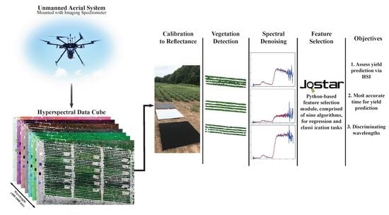
- Asses yield prediction of snap bean, at various points during the growing season, using hyperspectral imagery and descriptive models;
- Identify discriminating spectral features explaining yield; and
- Evaluate the most accurate time (growth period) for yield prediction, prior to harvest.
2. Methods
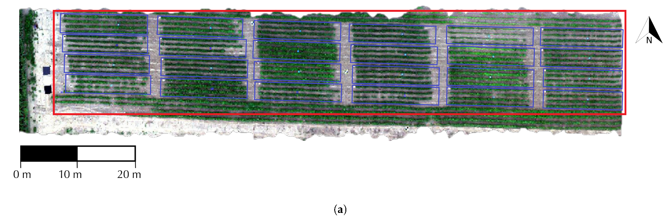
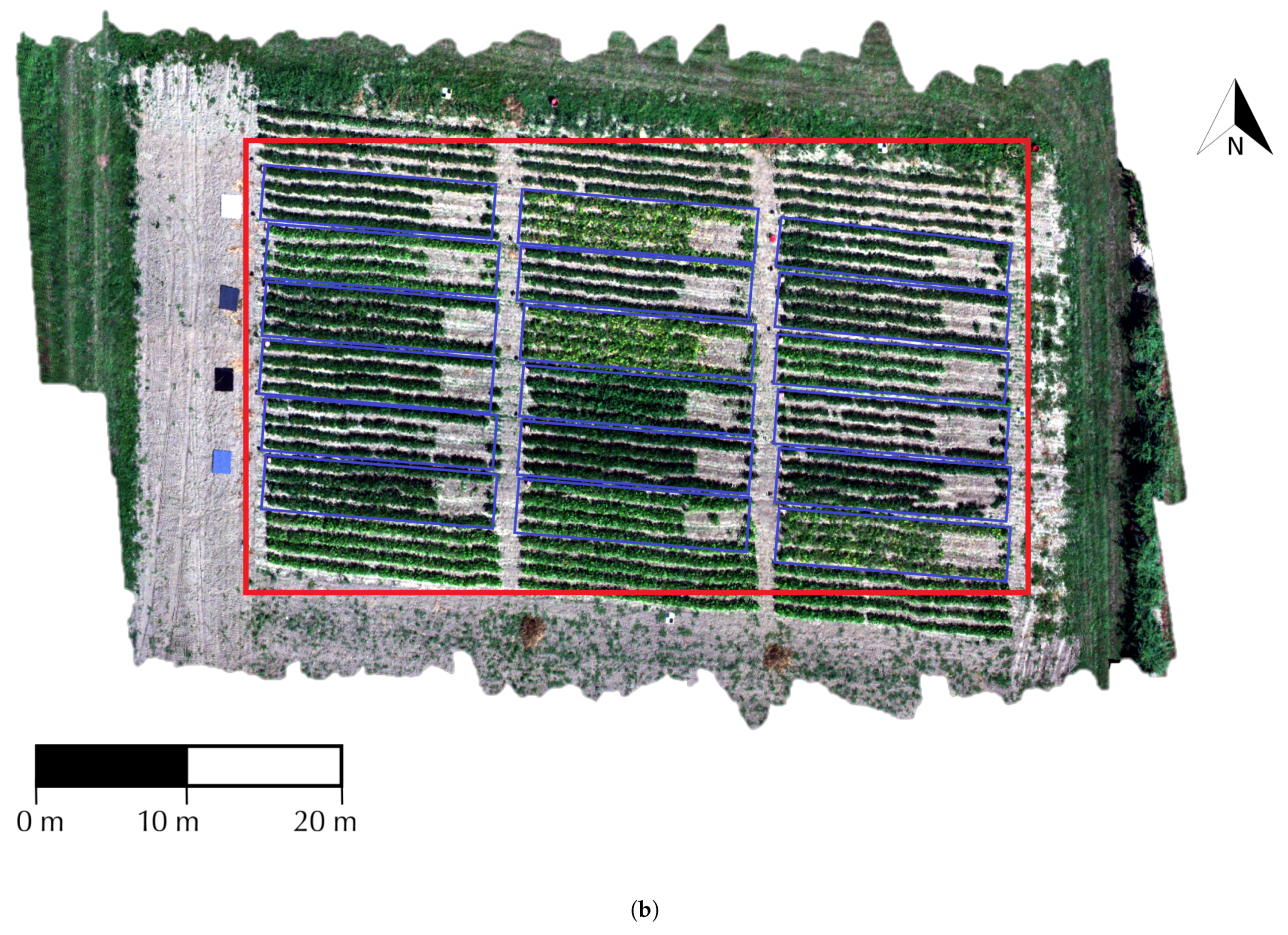
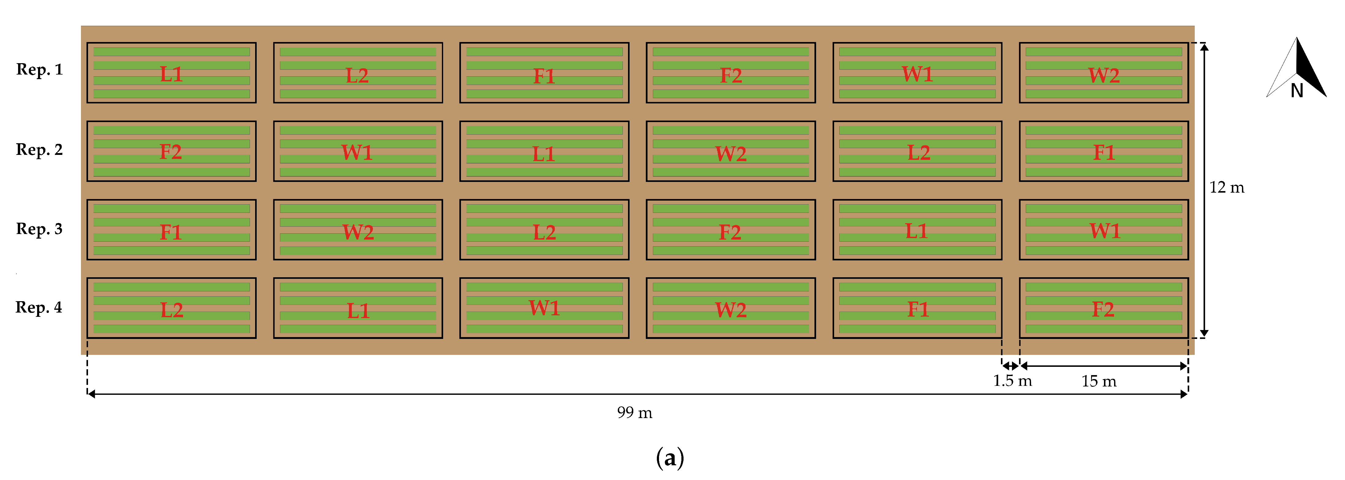
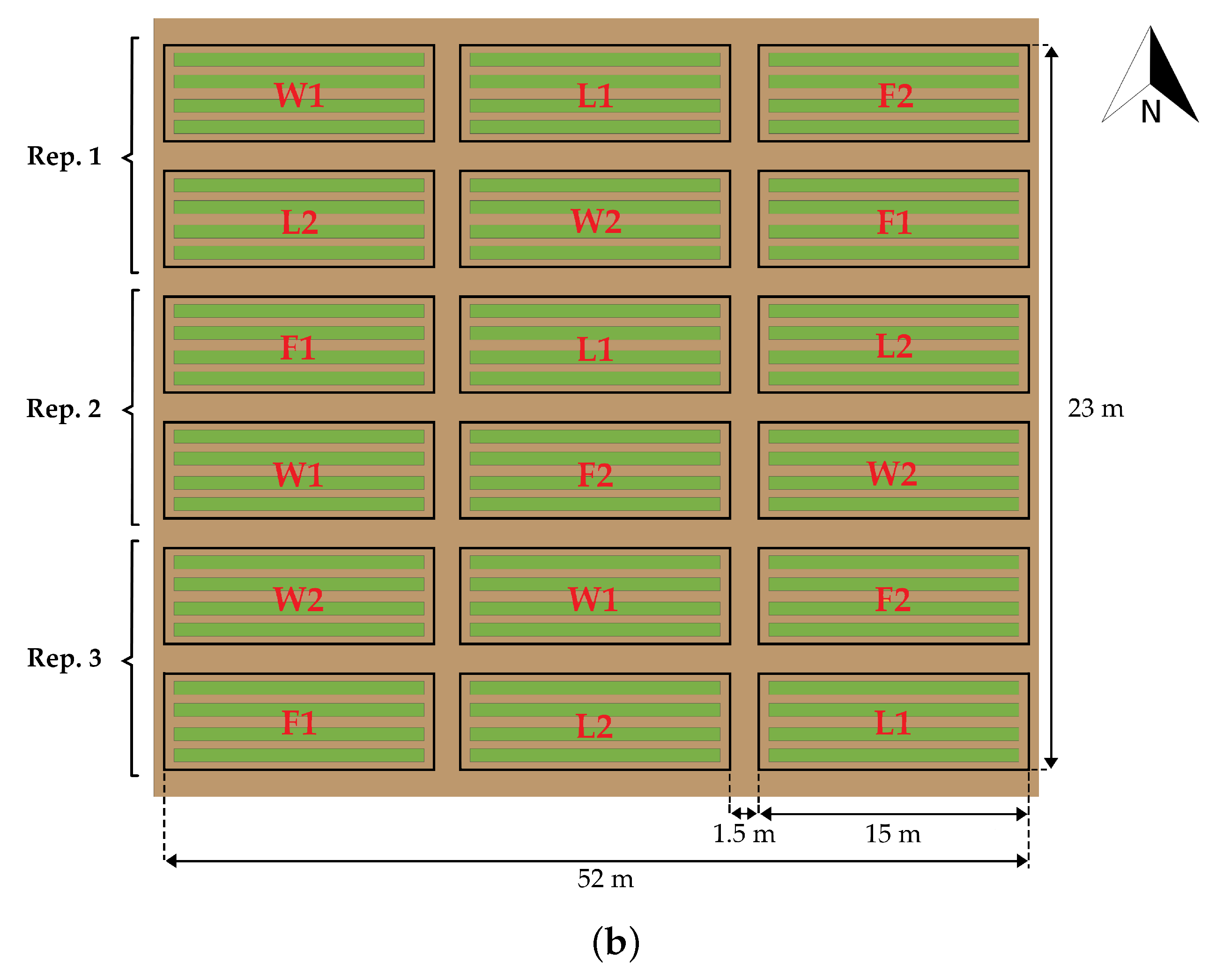
2.1. Study Area
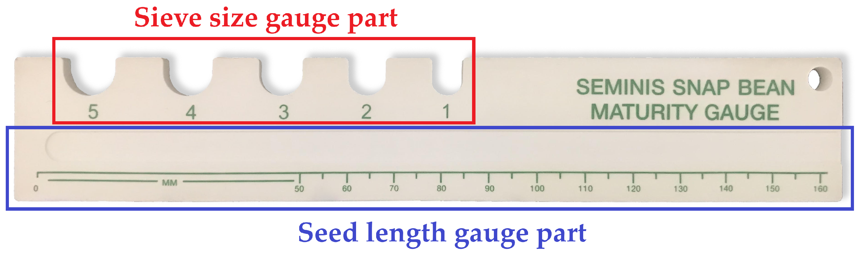
2.2. Assessment of Plant Growth Characteristics
2.3. Data Collection
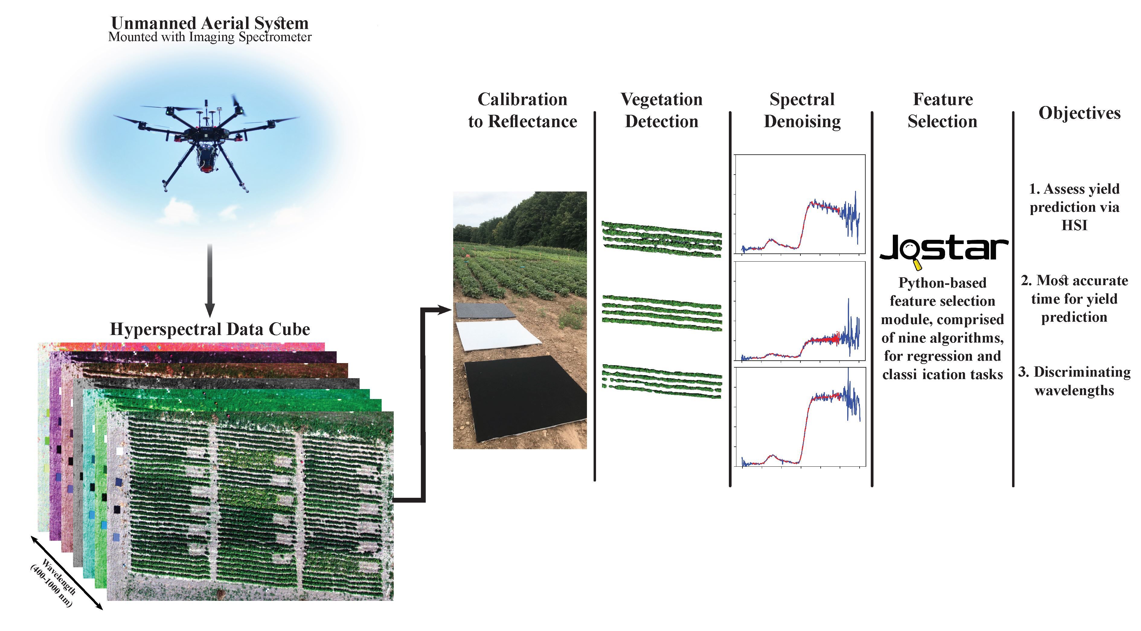
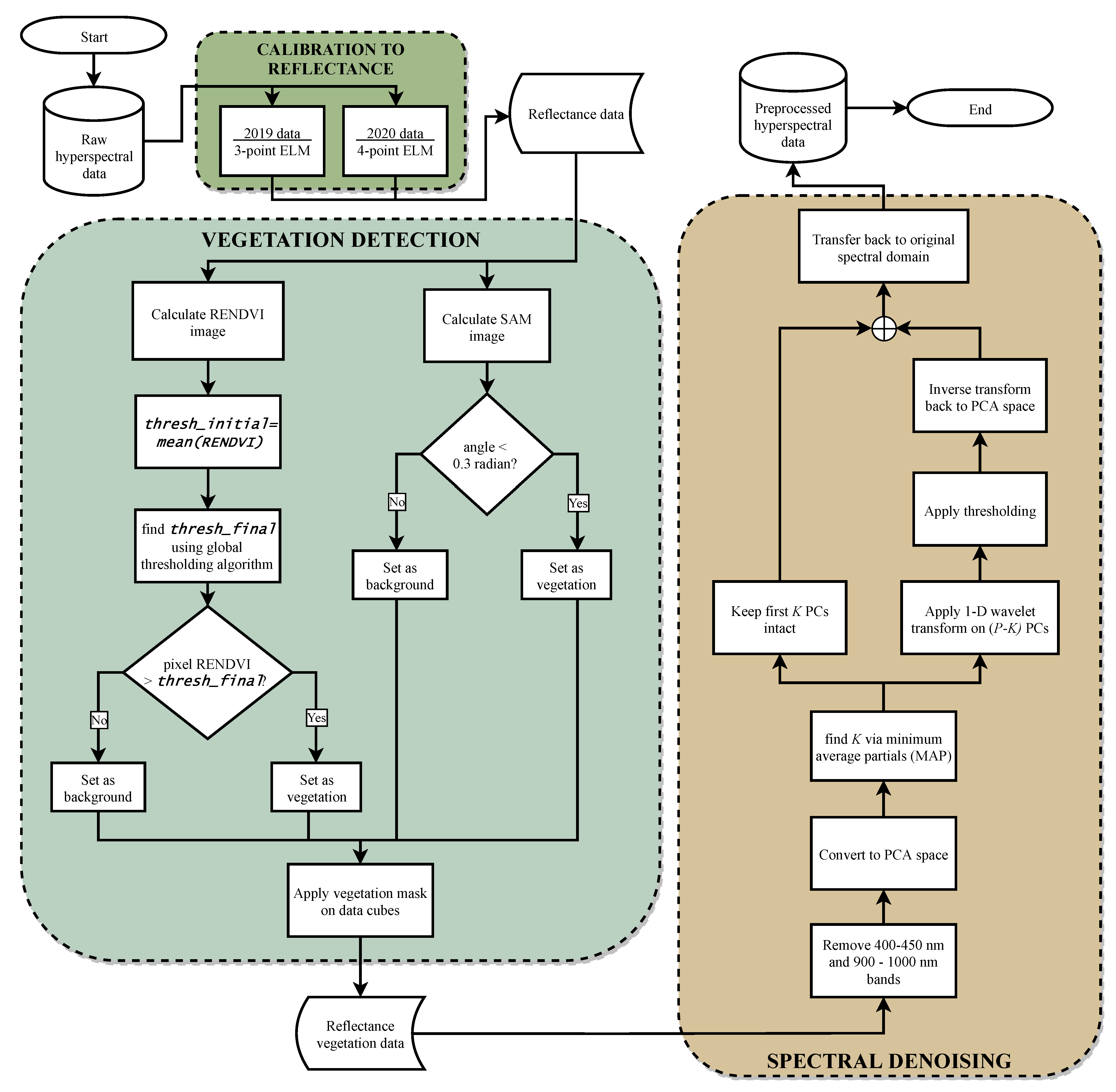
2.4. Data Preprocessing
2.4.1. Calibration to Reflectance
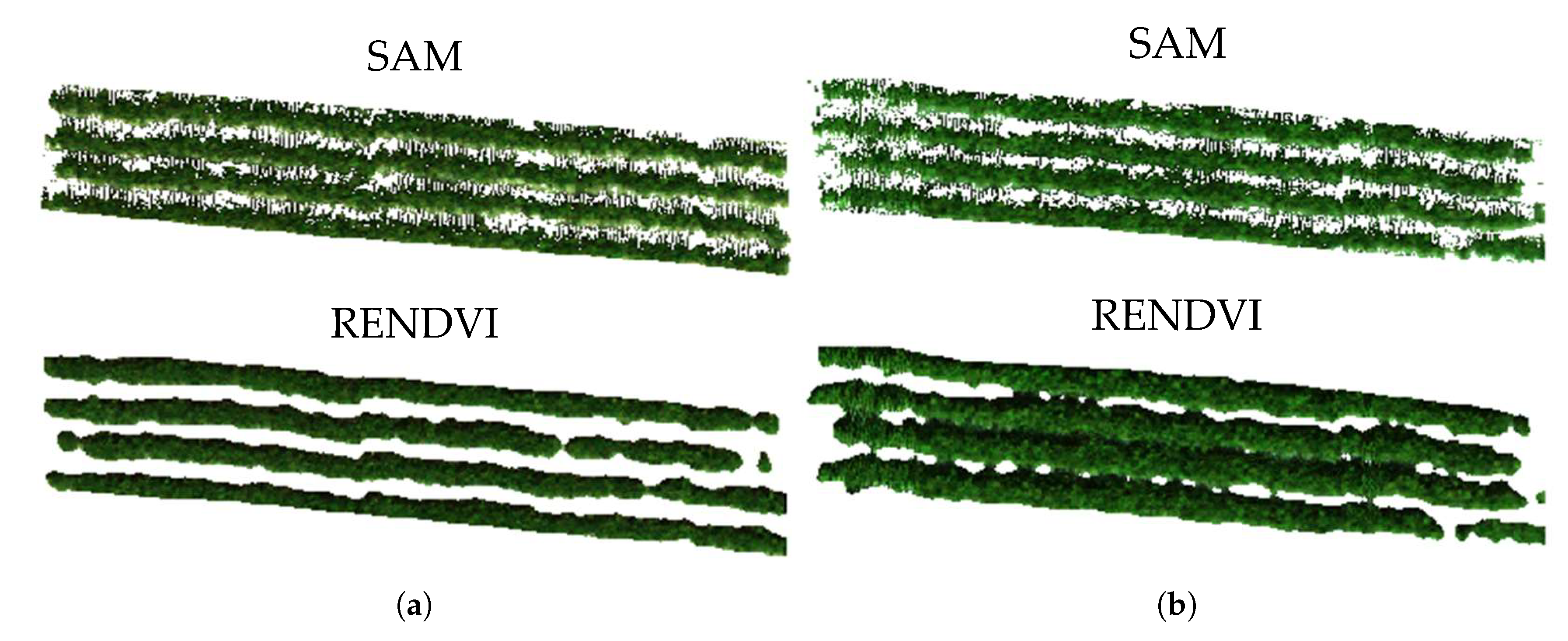
2.4.2. Vegetation Detection
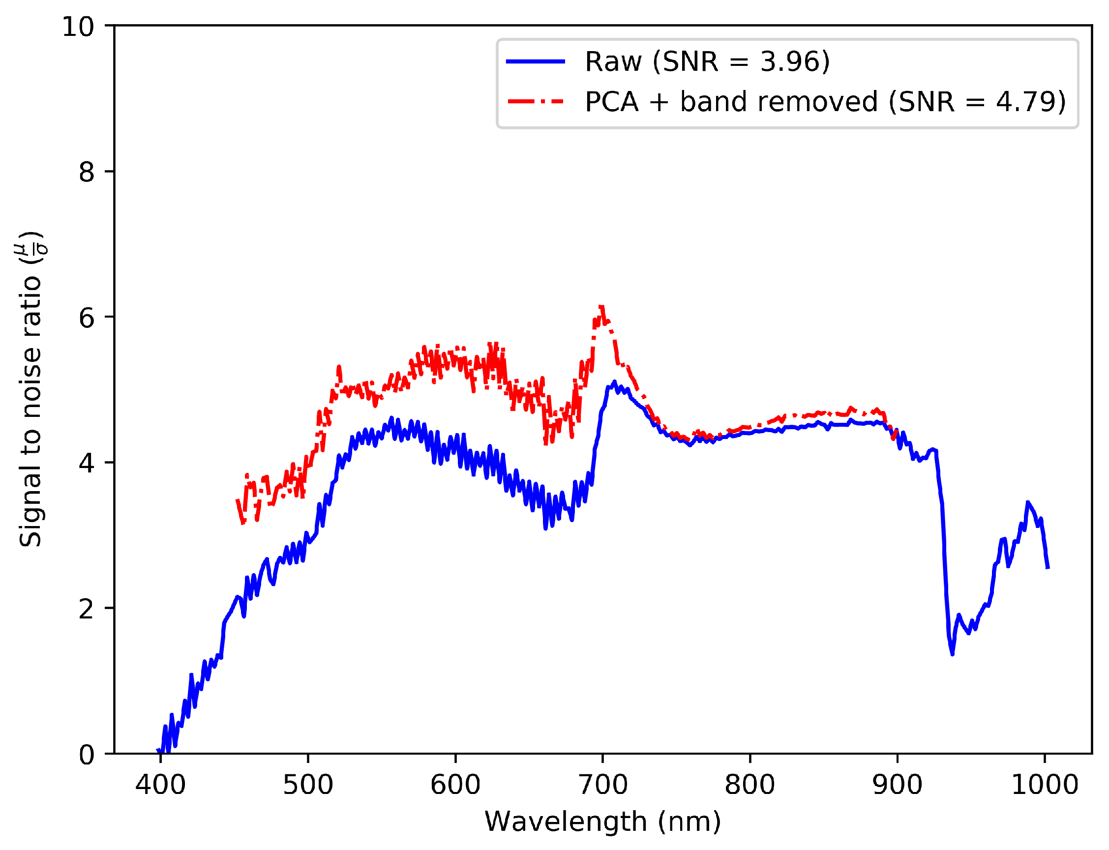
2.4.3. Spectral Denoising
2.5. Data Analysis
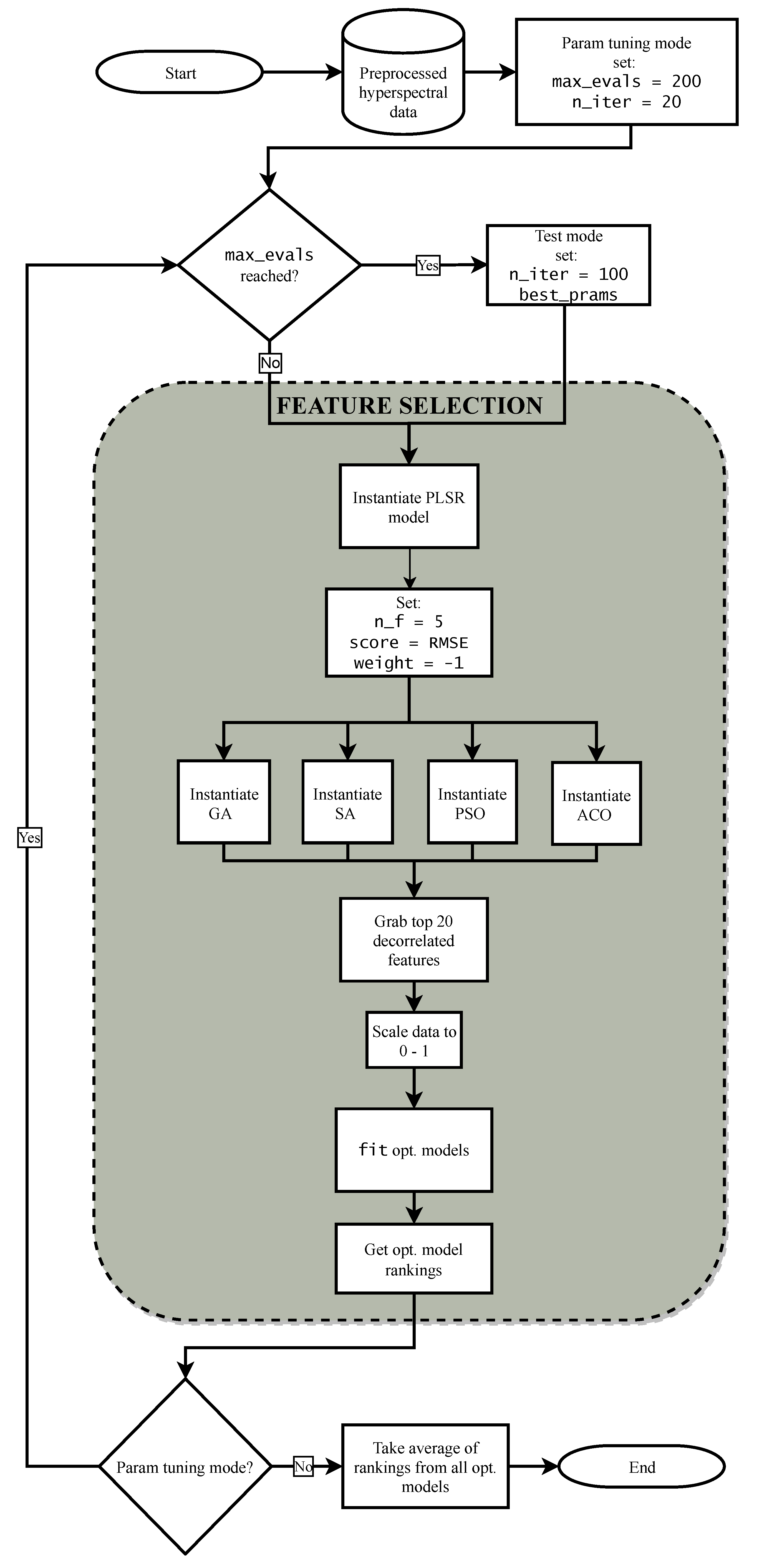
2.5.1. Jostar: Feature Selection Library in Python
2.5.2. Feature Selection Procedure
2.6. Software
3. Results
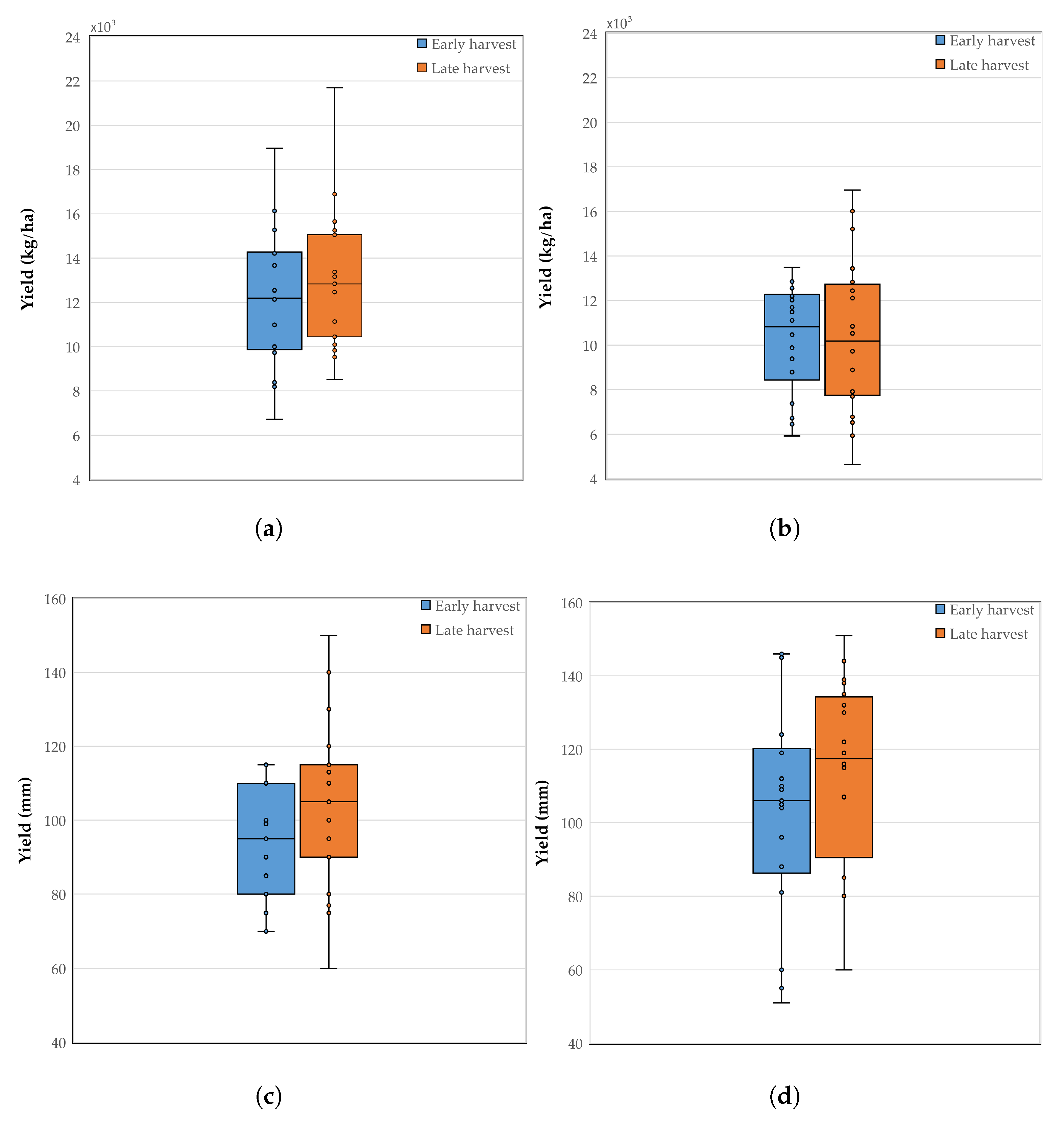
3.1. Descriptive Statistics
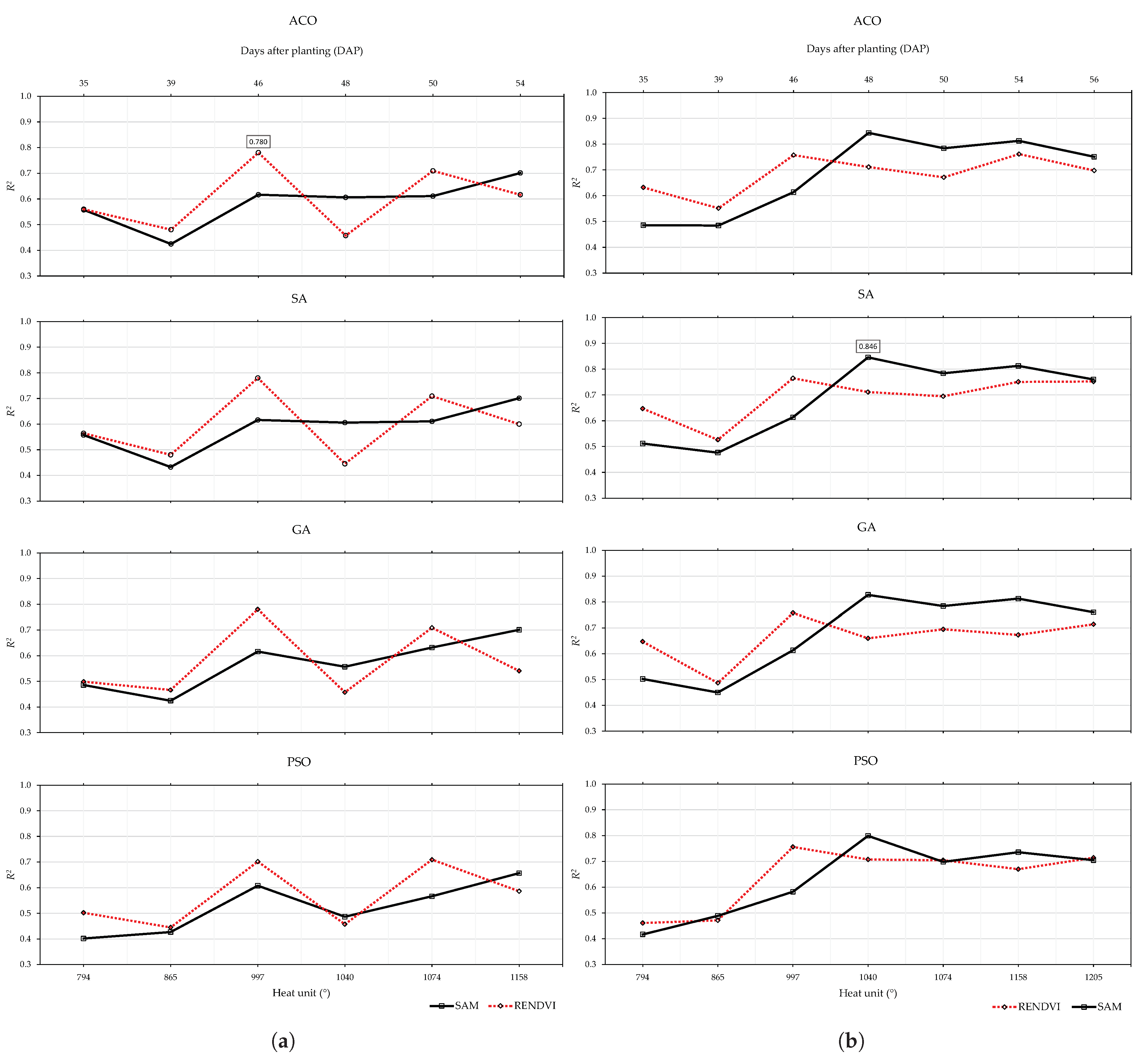
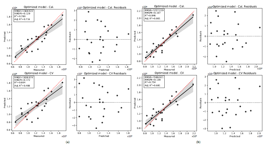
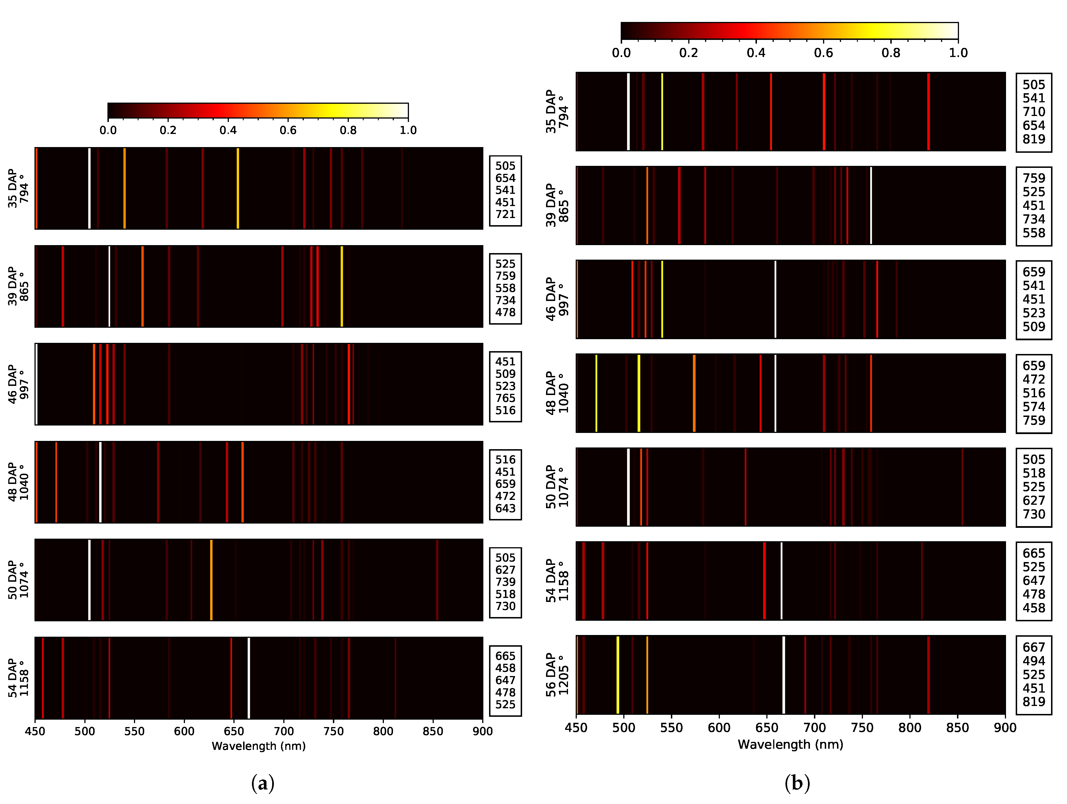
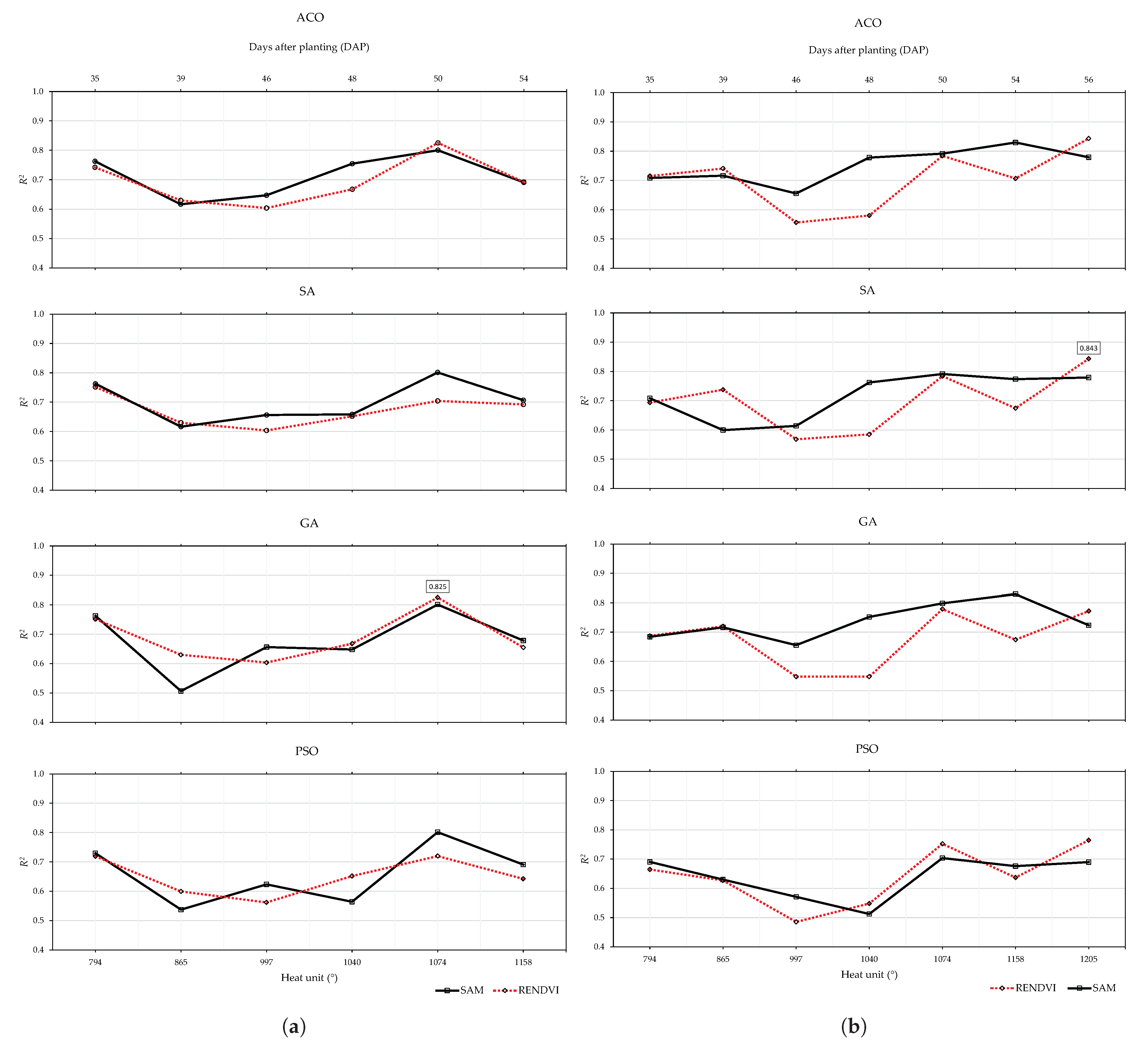
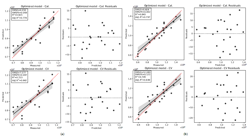
3.2. Pod Weight
3.2.1. 2019 Data Set
3.2.2. 2020 Data Set
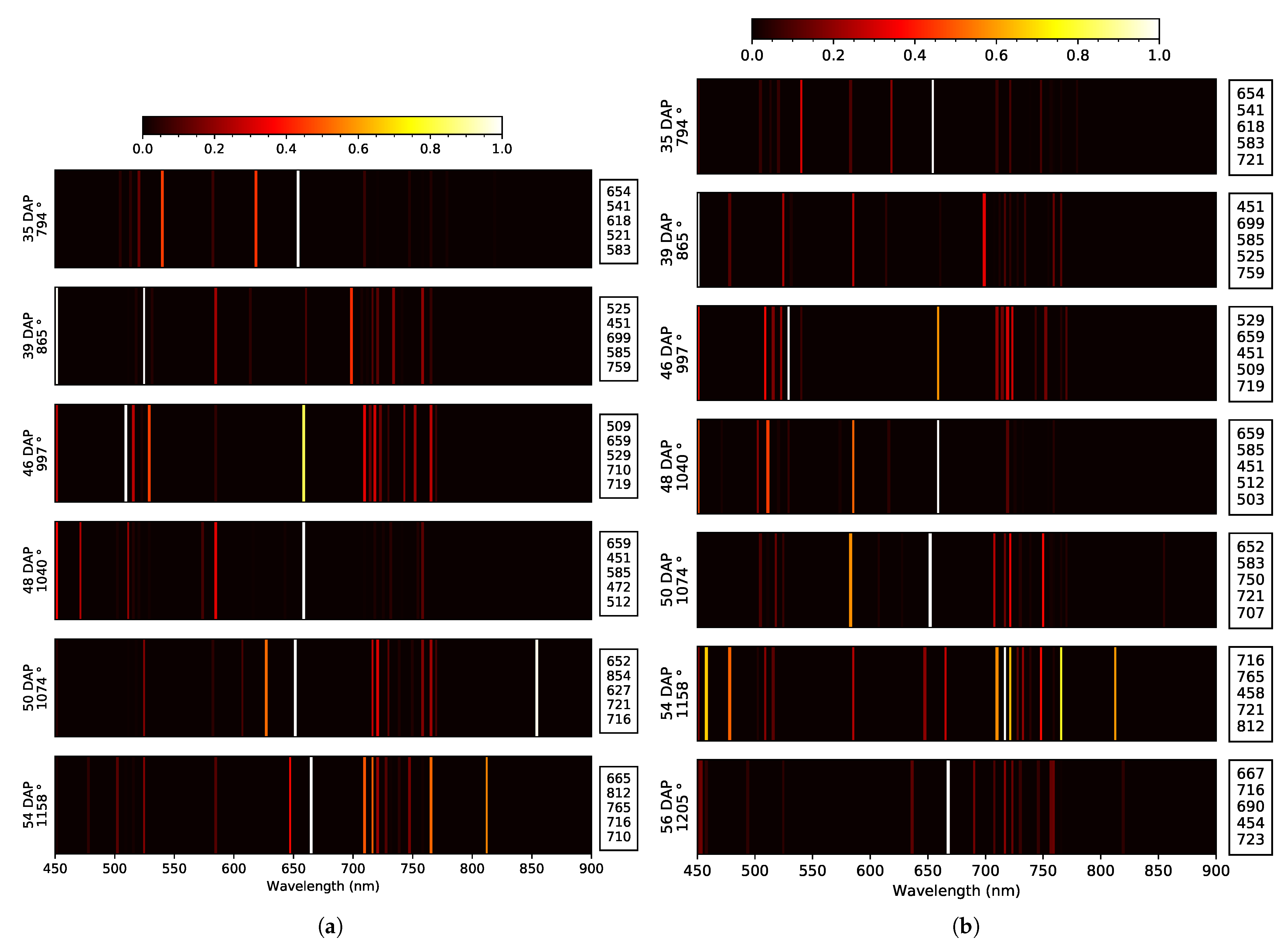
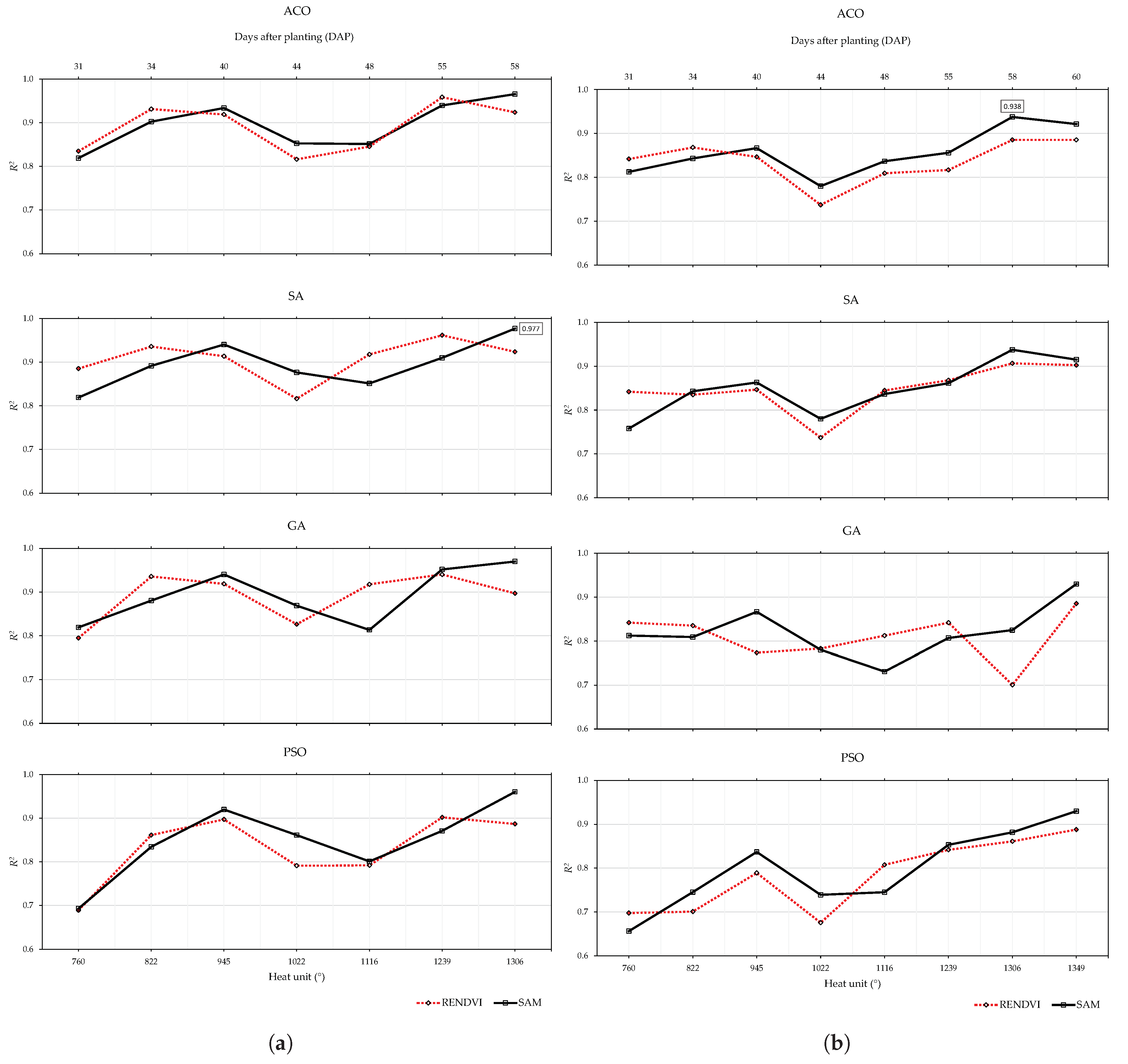
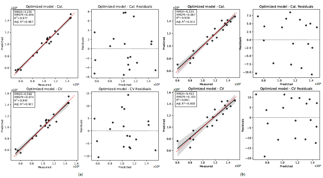
3.3. Seed Length
3.3.1. 2019 Data Set
3.3.2. 2020 Data Set
4. Discussion
5. Conclusions
Author Contributions
Funding
Institutional Review Board Statement
Informed Consent Statement
Data Availability Statement
Acknowledgments
Conflicts of Interest
Abbreviations
| ACO | ant colony optimization |
| DAP | days after planting |
| ELM | empirical line method |
| FWHM | full-width-half-maximum |
| GA | genetic algorithm |
| GDP | gross domestic product |
| GPU | graphics processing unit |
| GSD | ground sampling distance |
| KNN | K-nearest neighbors |
| LiDAR | light detection and ranging |
| LRS | plus-L minus-R |
| MAP | minimum average partial |
| NIR | near infrared |
| NSGAII | non-dominated sorting genetic algorithm-II |
| PA | precision agriculture |
| PC | principal component (PC) |
| PCA | principal component analysis |
| PLSR | partial least squares regression |
| PSO | particle Swarm Optimization |
| coefficient or determination | |
| RE | red edge |
| RENDVI | red-edge normalized difference vegetation index |
| RF | random forests |
| RFE | recursive feature elimination |
| root mean square error | |
| RS | remote sensing |
| SA | simulated annealing |
| SAM | spectral angle mapper |
| SBS | sequential backward search |
| SFS | sequential forward search |
| SVR | support vector regression |
| UAS | unmanned aerial systems |
| VIs | vegetation indices |
| VIS | visible |
References
- Ag and Food Sectors and the Economy. 2020. Available online: https://www.ers.usda.gov/data-products/ag-and-food-statistics-charting-the-essentials/ag-and-food-sectors-and-the-economy (accessed on 24 January 2021).
- Schellberg, J.; Hill, M.J.; Gerhards, R.; Rothmund, M.; Braun, M. Precision agriculture on grassland: Applications, perspectives and constraints. Eur. J. Agron. 2008, 29, 59–71. [Google Scholar] [CrossRef]
- Hassanzadeh, A.; van Aardt, J.; Murphy, S.P.; Pethybridge, S.J. Yield modeling of snap bean based on hyperspectral sensing: A greenhouse study. J. Appl. Remote Sens. 2020, 14, 024519. [Google Scholar] [CrossRef]
- Hassanzadeh, A.; Murphy, S.P.; Pethybridge, S.J.; van Aardt, J. Growth Stage Classification and Harvest Scheduling of Snap Bean Using Hyperspectral Sensing: A Greenhouse Study. Remote Sens. 2020, 12, 3809. [Google Scholar] [CrossRef]
- Elarab, M.; Ticlavilca, A.M.; Torres-Rua, A.F.; Maslova, I.; McKee, M. Estimating chlorophyll with thermal and broadband multispectral high resolution imagery from an unmanned aerial system using relevance vector machines for precision agriculture. Int. J. Appl. Earth Obs. Geoinf. 2015, 43, 32–42. [Google Scholar] [CrossRef] [Green Version]
- Yu, X.; Lu, H.; Liu, Q. Deep-learning-based regression model and hyperspectral imaging for rapid detection of nitrogen concentration in oilseed rape (Brassica napus L.) leaf. Chemom. Intell. Lab. Syst. 2018, 172, 188–193. [Google Scholar] [CrossRef]
- Tilling, A.K.; O’Leary, G.J.; Ferwerda, J.G.; Jones, S.D.; Fitzgerald, G.J.; Rodriguez, D.; Belford, R. Remote sensing of nitrogen and water stress in wheat. Field Crop. Res. 2007, 104, 77–85. [Google Scholar] [CrossRef]
- Thorp, K.; Tian, L. A review on remote sensing of weeds in agriculture. Precis. Agric. 2004, 5, 477–508. [Google Scholar] [CrossRef]
- Christy, C.D. Real-time measurement of soil attributes using on-the-go near infrared reflectance spectroscopy. Comput. Electron. Agric. 2008, 61, 10–19. [Google Scholar] [CrossRef]
- Lleó, L.; Barreiro, P.; Ruiz-Altisent, M.; Herrero, A. Multispectral images of peach related to firmness and maturity at harvest. J. Food Eng. 2009, 93, 229–235. [Google Scholar] [CrossRef] [Green Version]
- Lee, W.S.; Alchanatis, V.; Yang, C.; Hirafuji, M.; Moshou, D.; Li, C. Sensing technologies for precision specialty crop production. Comput. Electron. Agric. 2010, 74, 2–33. [Google Scholar] [CrossRef]
- Mulla, D.J. Twenty five years of remote sensing in precision agriculture: Key advances and remaining knowledge gaps. Biosyst. Eng. 2013, 114, 358–371. [Google Scholar] [CrossRef]
- Schwalbert, R.A.; Amado, T.; Corassa, G.; Pott, L.P.; Prasad, P.V.; Ciampitti, I.A. Satellite-based soybean yield forecast: Integrating machine learning and weather data for improving crop yield prediction in southern Brazil. Agric. For. Meteorol. 2020, 284, 107886. [Google Scholar] [CrossRef]
- Li, B.; Xu, X.; Zhang, L.; Han, J.; Bian, C.; Li, G.; Liu, J.; Jin, L. Above-ground biomass estimation and yield prediction in potato by using UAV-based RGB and hyperspectral imaging. ISPRS J. Photogramm. Remote Sens. 2020, 162, 161–172. [Google Scholar] [CrossRef]
- Feng, L.; Zhang, Z.; Ma, Y.; Du, Q.; Williams, P.; Drewry, J.; Luck, B. Alfalfa Yield Prediction Using UAV-Based Hyperspectral Imagery and Ensemble Learning. Remote Sens. 2020, 12, 2028. [Google Scholar] [CrossRef]
- Nasrabadi, N.M. Hyperspectral target detection: An overview of current and future challenges. IEEE Signal Process. Mag. 2013, 31, 34–44. [Google Scholar] [CrossRef]
- Im, J.; Jensen, J.R. Hyperspectral remote sensing of vegetation. Geogr. Compass 2008, 2, 1943–1961. [Google Scholar] [CrossRef]
- Curran, P.J. Remote sensing of foliar chemistry. Remote Sens. Environ. 1989, 30, 271–278. [Google Scholar] [CrossRef]
- Plaza, J.; Plaza, A.; Perez, R.; Martinez, P. On the use of small training sets for neural network-based characterization of mixed pixels in remotely sensed hyperspectral images. Pattern Recognition 2009, 42, 3032–3045. [Google Scholar] [CrossRef]
- Rasti, B.; Scheunders, P.; Ghamisi, P.; Licciardi, G.; Chanussot, J. Noise reduction in hyperspectral imagery: Overview and application. Remote Sens. 2018, 10, 482. [Google Scholar] [CrossRef] [Green Version]
- Yuan, Q.; Zhang, L.; Shen, H. Hyperspectral image denoising employing a spectral–spatial adaptive total variation model. IEEE Trans. Geosci. Remote Sens. 2012, 50, 3660–3677. [Google Scholar] [CrossRef]
- Kerekes, J.P.; Baum, J.E. Hyperspectral imaging system modeling. Linc. Lab. J. 2003, 14, 117–130. Available online: https://www.cis.rit.edu/people/faculty/kerekes/pdfs/LLJ_2003_Kerekes.pdf (accessed on 24 January 2021).
- Griffin, M.K.; Burke, H.H.K. Compensation of hyperspectral data for atmospheric effects. Linc. Lab. J. 2003, 14, 29–54. Available online: https://129.55.110.66/publications/journal/pdf/vol14_no1/14_1compensation.pdf (accessed on 24 January 2021).
- Antczak, K. Deep recurrent neural networks for ECG signal denoising. arXiv 2018, arXiv:1807.11551. Available online: https://arxiv.org/abs/1807.11551v3 (accessed on 24 January 2021).
- Jiang, Y.; Li, H.; Rangaswamy, M. Deep learning denoising based line spectral estimation. IEEE Signal Process. Lett. 2019, 26, 1573–1577. [Google Scholar] [CrossRef]
- Zhang, C.; Zhou, L.; Zhao, Y.; Zhu, S.; Liu, F.; He, Y. Noise reduction in the spectral domain of hyperspectral images using denoising autoencoder methods. Chemom. Intell. Lab. Syst. 2020, 203, 104063. [Google Scholar] [CrossRef]
- Schulze, G.; Jirasek, A.; Marcia, M.; Lim, A.; Turner, R.F.; Blades, M.W. Investigation of selected baseline removal techniques as candidates for automated implementation. Appl. Spectrosc. 2005, 59, 545–574. [Google Scholar] [CrossRef]
- Chen, Y.; Oliver, D.S.; Zhang, D. Data assimilation for nonlinear problems by ensemble Kalman filter with reparameterization. J. Pet. Sci. Eng. 2009, 66, 1–14. [Google Scholar] [CrossRef]
- Fernández-Novales, J.; López, M.I.; Sánchez, M.T.; Morales, J.; González-Caballero, V. Shortwave-near infrared spectroscopy for determination of reducing sugar content during grape ripening, winemaking, and aging of white and red wines. Food Res. Int. 2009, 42, 285–291. [Google Scholar] [CrossRef]
- Lang, M.; Guo, H.; Odegard, J.E.; Burrus, C.S.; Wells, R.O. Noise reduction using an undecimated discrete wavelet transform. IEEE Signal Process. Lett. 1996, 3, 10–12. [Google Scholar] [CrossRef]
- Jansen, M. Noise Reduction by Wavelet Thresholding; Springer Science & Business Media: Berlin/Heidelberg, Germany, 2012; Volume 161. [Google Scholar] [CrossRef]
- Chen, G.; Qian, S.E. Denoising of hyperspectral imagery using principal component analysis and wavelet shrinkage. IEEE Trans. Geosci. Remote Sens. 2010, 49, 973–980. [Google Scholar] [CrossRef]
- Zwick, W.R.; Velicer, W.F. Comparison of five rules for determining the number of components to retain. Psychol. Bull. 1986, 99, 432. Available online: https://files.eric.ed.gov/fulltext/ED251510.pdf (accessed on 24 January 2021). [CrossRef]
- Bartlett, M.S. Tests of significance in factor analysis. Br. J. Stat. Psychol. 1950, 3, 77–85. [Google Scholar] [CrossRef]
- Kaiser, H.F. The application of electronic computers to factor analysis. Educ. Psychol. Meas. 1960, 20, 141–151. [Google Scholar] [CrossRef]
- Velicer, W.F. The relation between factor score estimates, image scores, and principal component scores. Educ. Psychol. Meas. 1976, 36, 149–159. [Google Scholar] [CrossRef]
- Cattell, R.B. The scree test for the number of factors. Multivar. Behav. Res. 1966, 1, 245–276. [Google Scholar] [CrossRef] [PubMed]
- Horn, J.L. A rationale and test for the number of factors in factor analysis. Psychometrika 1965, 30, 179–185. [Google Scholar] [CrossRef] [PubMed]
- Hang, R.; Liu, Q.; Hong, D.; Ghamisi, P. Cascaded recurrent neural networks for hyperspectral image classification. IEEE Trans. Geosci. Remote Sens. 2019, 57, 5384–5394. [Google Scholar] [CrossRef] [Green Version]
- Agarwal, A.; El-Ghazawi, T.; El-Askary, H.; Le-Moigne, J. Efficient hierarchical-PCA dimension reduction for hyperspectral imagery. In Proceedings of the 2007 IEEE International Symposium on Signal Processing and Information Technology, Giza, Egypt, 15–18 December 2007; pp. 353–356. [Google Scholar] [CrossRef]
- Benesty, J.; Chen, J.; Huang, Y.; Cohen, I. Pearson correlation coefficient. In Noise Reduction in Speech Processing; Springer: Berlin/Heidelberg, Germany, 2009; pp. 1–4. [Google Scholar] [CrossRef]
- Hawkins, D.M. The problem of overfitting. J. Chem. Inf. Comput. Sci. 2004, 44, 1–12. [Google Scholar] [CrossRef] [PubMed]
- Venkatesh, B.; Anuradha, J. A review of feature selection and its methods. Cybern. Inf. Technol. 2019, 19, 3–26. [Google Scholar] [CrossRef] [Green Version]
- Pearson, K. LIII. On lines and planes of closest fit to systems of points in space. London Edinburgh Dublin Philos. Mag. J. Sci. 1901, 2, 559–572. [Google Scholar] [CrossRef] [Green Version]
- Battiti, R. Using mutual information for selecting features in supervised neural net learning. IEEE Trans. Neural Netw. 1994, 5, 537–550. [Google Scholar] [CrossRef] [Green Version]
- Kumar, V.; Minz, S. Feature selection: A literature review. SmartCR 2014, 4, 211–229. [Google Scholar] [CrossRef]
- Goldenberg, D.E. Genetic Algorithms in Search, Optimization and Machine Learning. 1989. Available online: https://deepblue.lib.umich.edu/bitstream/handle/2027.42/46947/10994_2005_Article_422926.pdf (accessed on 24 January 2021).
- Li, B.; Wang, L.; Song, W. Ant colony optimization for the traveling salesman problem based on ants with memory. In Proceedings of the 2008 Fourth International Conference on Natural Computation, Jinan, China, 18–20 October 2008; Volume 7, pp. 496–501. [Google Scholar] [CrossRef]
- Del Valle, Y.; Venayagamoorthy, G.K.; Mohagheghi, S.; Hernandez, J.C.; Harley, R.G. Particle swarm optimization: Basic concepts, variants and applications in power systems. IEEE Trans. Evol. Comput. 2008, 12, 171–195. [Google Scholar] [CrossRef]
- John, G.H.; Kohavi, R.; Pfleger, K. Irrelevant features and the subset selection problem. In Machine Learning Proceedings 1994; Elsevier: Amsterdam, The Netherlands, 1994; pp. 121–129. [Google Scholar] [CrossRef]
- Ma, S.; Huang, J. Penalized feature selection and classification in bioinformatics. Briefings Bioinform. 2008, 9, 392–403. [Google Scholar] [CrossRef] [Green Version]
- Tao, H.; Feng, H.; Xu, L.; Miao, M.; Yang, G.; Yang, X.; Fan, L. Estimation of the yield and plant height of winter wheat using UAV-based hyperspectral images. Sensors 2020, 20, 1231. [Google Scholar] [CrossRef] [Green Version]
- USDA. USDA National Agricultural Statistics Service; National Statistical Services. 2016. Available online: https://quickstats.nass.usda.gov/results/5B4DC16F-4537-38BB-86AC-010B3FBF83DC?pivot=short_desc (accessed on 24 January 2021).
- Yuan, M.; Ruark, M.D.; Bland, W.L. A simple model for snap bean (Phaseolus vulgaris L.) development, growth and yield in response to nitrogen. Field Crop. Res. 2017, 211, 125–136. [Google Scholar] [CrossRef]
- Saleh, S.; Liu, G.; Liu, M.; Ji, Y.; He, H.; Gruda, N. Effect of Irrigation on Growth, Yield, and Chemical Composition of Two Green Bean Cultivars. Horticulturae 2018, 4, 3. [Google Scholar] [CrossRef] [Green Version]
- Kaputa, D.S.; Bauch, T.; Roberts, C.; McKeown, D.; Foote, M.; Salvaggio, C. Mx-1: A new multi-modal remote sensing uas payload with high accuracy gps and imu. In Proceedings of the 2019 IEEE Systems and Technologies for Remote Sensing Applications Through Unmanned Aerial Systems (STRATUS), Rochester, NY, USA, 25–27 February 2019; pp. 1–4. [Google Scholar] [CrossRef]
- Mamaghani, B.; Salvaggio, C. Comparative study of panel and panelless-based reflectance conversion techniques for agricultural remote sensing. arXiv 2019, arXiv:1910.03734. Available online: https://arxiv.org/abs/1910.03734 (accessed on 24 January 2021).
- Lee, S.U.; Chung, S.Y.; Park, R.H. A comparative performance study of several global thresholding techniques for segmentation. Comput. Vision Graph. Image Process. 1990, 52, 171–190. [Google Scholar] [CrossRef]
- Yuhas, R.H.; Goetz, A.F.; Boardman, J.W. Discrimination among semi-arid landscape endmembers using the spectral angle mapper (SAM) algorithm. In Proceedings of the Summaries 3rd Annual JPL Airborne Geoscience Workshop, Pasadena, CA, USA, 1–5 June 1992; Volume 1, pp. 147–149. [Google Scholar]
- Garrido, L.E.; Abad, F.J.; Ponsoda, V. Performance of Velicer’s minimum average partial factor retention method with categorical variables. Educ. Psychol. Meas. 2011, 71, 551–570. [Google Scholar] [CrossRef]
- Price, K.V. Differential evolution. In Handbook of Optimization; Springer: Berlin/Heidelberg, Germany, 2013; pp. 187–214. [Google Scholar] [CrossRef]
- Van Laarhoven, P.J.; Aarts, E.H. Simulated annealing. In Simulated Annealing: Theory and Applications; Springer: Berlin/Heidelberg, Germany, 1987; pp. 7–15. [Google Scholar] [CrossRef]
- Levin, L.A. Universal sequential search problems. Probl. Peredachi Inform. 1973, 9, 115–116. Available online: http://www.mathnet.ru/links/e8c7e04918539cbbc30a0f5ff178abdc/ppi914.pdf (accessed on 24 January 2021).
- Deb, K.; Pratap, A.; Agarwal, S.; Meyarivan, T. A fast and elitist multiobjective genetic algorithm: NSGA-II. IEEE Trans. Evol. Comput. 2002, 6, 182–197. [Google Scholar] [CrossRef] [Green Version]
- Altmann, A.; Toloşi, L.; Sander, O.; Lengauer, T. Permutation importance: A corrected feature importance measure. Bioinformatics 2010, 26, 1340–1347. [Google Scholar] [CrossRef]
- Van Rossum, G.; Drake, F.L., Jr. Python Tutorial; Centrum voor Wiskunde en Informatica: Amsterdam, The Netherlands, 1995; Available online: http://lib.21h.io/library/G7B3RFY7/download/GBMFTU3C/Python_3.8.3_Docs_.pdf (accessed on 24 January 2021).
- Bergstra, J.; Yamins, D.; Cox, D.D. Hyperopt: A python library for optimizing the hyperparameters of machine learning algorithms. In Proceedings of the 12th Python in Science Conference, Citeseer, Austin, TX, USA, 12–18 July 2013; Volume 13, p. 20. Available online: http://citeseerx.ist.psu.edu/viewdoc/download?doi=10.1.1.704.3494&rep=rep1&type=pdf (accessed on 24 January 2021).
- Pedregosa, F.; Varoquaux, G.; Gramfort, A.; Michel, V.; Thirion, B.; Grisel, O.; Blondel, M.; Prettenhofer, P.; Weiss, R.; Dubourg, V.; et al. Scikit-learn: Machine learning in Python. J. Mach. Learn. Res. 2011, 12, 2825–2830. [Google Scholar]
- Bajorski, P. Statistics for Imaging, Optics, and Photonics; John Wiley & Sons: Hoboken, NJ, USA, 2011; Volume 808. [Google Scholar] [CrossRef]
- Wei, F.; Yan, Z.; Yongchao, T.; Weixing, C.; Xia, Y.; Yingxue, L. Monitoring leaf nitrogen accumulation in wheat with hyper-spectral remote sensing. Acta Ecol. Sin. 2008, 28, 23–32. [Google Scholar] [CrossRef]
- Sims, D.A.; Gamon, J.A. Relationships between leaf pigment content and spectral reflectance across a wide range of species, leaf structures and developmental stages. Remote Sens. Environ. 2002, 81, 337–354. [Google Scholar] [CrossRef]
- Adão, T.; Hruška, J.; Pádua, L.; Bessa, J.; Peres, E.; Morais, R.; Sousa, J.J. Hyperspectral imaging: A review on UAV-based sensors, data processing and applications for agriculture and forestry. Remote Sens. 2017, 9, 1110. [Google Scholar] [CrossRef] [Green Version]
- Zhao, D.; Reddy, K.R.; Kakani, V.G.; Read, J.J.; Koti, S. Canopy reflectance in cotton for growth assessment and lint yield prediction. Eur. J. Agron. 2007, 26, 335–344. [Google Scholar] [CrossRef]
- Hassan, M.A.; Yang, M.; Rasheed, A.; Yang, G.; Reynolds, M.; Xia, X.; Xiao, Y.; He, Z. A rapid monitoring of NDVI across the wheat growth cycle for grain yield prediction using a multi-spectral UAV platform. Plant Sci. 2019, 282, 95–103. [Google Scholar] [CrossRef]


| Model | Date | Stage | Days after Planting (DAP) | Heat Unit () * | GSD (cm) |
|---|---|---|---|---|---|
| 2019 | 06/27/2019 | Sowing | 0 | 0 | N/A |
| 08/01/2019 | Flowering | 35 | 794 | 3 | |
| 08/05/2019 | Flowering | 39 | 865 | 3 | |
| 08/12/2019 | Pod formation | 46 | 997 | 1.5 | |
| 08/14/2019 | Pod formation | 48 | 1040 | 3 | |
| 08/16/2019 | Pod formation | 50 | 1074 | 3 | |
| 08/20/2019 | Pod formation (early harvest) | 54 | 1158 | 3 | |
| 08/22/2019 | Pod formation (late harvest) | 56 | 1205 | 3 | |
| 2020 | 06/27/2020 | Sowing | 0 | 0 | N/A |
| 07/28/2020 | Budding | 31 | 760 | 3 | |
| 07/31/2020 | Flowering | 34 | 822 | 3 | |
| 08/06/2020 | Flowering | 40 | 945 | 3 | |
| 08/10/2020 | Pod formation | 44 | 1022 | 3 | |
| 08/14/2020 | Pod formation | 48 | 1116 | 3 | |
| 08/21/2020 | Pod formation | 55 | 1239 | 3 | |
| 08/24/2020 | Pod formation (early harvest) | 58 | 1306 | 3 | |
| 08/26/2020 | Pod formation (late harvest) | 60 | 1346 | 3 |
| Optimization Model | Parameter | Description | Sampling Method | Low Bound | High Bound |
|---|---|---|---|---|---|
| GA | Crossover percentage | Uniform logarithmic | 0.5 | ||
| Mutation percentage | Uniform logarithmic | 0.2 | |||
| Mutation rate | Uniform logarithmic | 0.2 | |||
| Selection pressure | Random integer | 1 | 10 | ||
| Population size | Random integer | 20 | 200 | ||
| SA | Cooling factor | Uniform logarithmic | 0.8 | 0.99 | |
| Initial temperature | Uniform logarithmic | 500 | |||
| Number of sub-iterations | Random Integer | 20 | 200 | ||
| PSO | Information elicitation factor | Uniform logarithmic | 0.5 | ||
| Cognitive parameter | Uniform logarithmic | 2 | |||
| Social parameter | Uniform logarithmic | 2 | |||
| W | Inertia weight | Uniform logarithmic | 1.2 | ||
| Inertia weight damping factor | Uniform logarithmic | 0.5 | |||
| Number of particles | Random integer | 20 | 200 | ||
| ACO | Information elicitation factor | Uniform logarithmic | 0.5 | ||
| Pheromone evaporation coefficient | Uniform logarithmic | 0.5 | |||
| Initial pheromone intensity | Uniform logarithmic | 1 | |||
| Q | Pheromone intensity | Uniform logarithmic | 1 | ||
| Number of ants | Random integer | 20 | 200 | ||
| Meta-heuristic factor | Random integer | 1 | 5 |
| Data Set | Yield Indicator | Across Yield Indicator WL (nm) Similarity | |||||
|---|---|---|---|---|---|---|---|
| Pod Weight | Seed Length | ||||||
| Zone (DAP) | WL (nm) | Dip | Zone (DAP) | WL (nm) | Dip | ||
| 2019 early | Blue: E. 50 Green: T. Red: E. 39, 46 RE: E. 48, 54 NIR: NA | 3x: 451 2x: 478, 505, 516, 525 | at 39 DAP None | Blue: E. 39, 48 Green: E. 50, 54 Red: T. RE: E. 35, 48 NIR: O. e 50, 54 | 2x: 451, 585, 659, 710, 716 | at 40 DAP at 55 DAP | 451 |
| 2019 late | Blue: E. 35, 50 Green: T. Red: E. 39 RE: E. 46, 54, 56 NIR: O. 35, 56 | 4x: 525 3x: 451 2x: 505, 541, 659, 759, 819 | None at 56 DAP | Blue: E. 35, 50 Green: E. 54, 56 Red: E. 54 RE: O. 48 NIR: O. 54 | 3x: 451, 721 2x: 583, 585, 659, 716 | at 46 DAP at 56 DAP | 451, 659 |
| 2020 early | Blue: T. Green: E. 44 Red: E. 58 RE: T. NIR: NA | 5x: 451, 759 3x: 523 2x: 518, 607, 647 | at 34 DAP at 55 DAP | Blue: T. Green: E. 58 Red: E. 44, 55, 58 RE: E. 31, 48 NIR: O. 58 | 6x: 451 2x: 494, 518 | at 44 DAP None | 451, 518 |
| 2020 late | Blue: E. 58 Green: E. 44 Red: E. 40 RE: E. 31, 55, 60 NIR: NA | 4x: 451, 756 2x: 474, 500, 525, 654, 707 | at 34 DAP at 60 DAP | Blue: T. Green: E. 58 Red: E. 58, 60 RE: E. 31, 34 NIR: O. 58 | 7x: 451 2x: 494, 518, 670, 699, 759 | at 44 DAP at 60 DAP | 451, ∼500, ∼520, ∼700, ∼760 |
| Across years WL (nm) similarity | 451, ∼500, ∼ 520, ∼650, ∼760 | 451, ∼520, ∼500, ∼585, ∼660, ∼720 | ∼451, ∼500, ∼520, ∼650, ∼700, ∼760 | ||||
Publisher’s Note: MDPI stays neutral with regard to jurisdictional claims in published maps and institutional affiliations. |
© 2021 by the authors. Licensee MDPI, Basel, Switzerland. This article is an open access article distributed under the terms and conditions of the Creative Commons Attribution (CC BY) license (https://creativecommons.org/licenses/by/4.0/).
Share and Cite
Hassanzadeh, A.; Zhang, F.; van Aardt, J.; Murphy, S.P.; Pethybridge, S.J. Broadacre Crop Yield Estimation Using Imaging Spectroscopy from Unmanned Aerial Systems (UAS): A Field-Based Case Study with Snap Bean. Remote Sens. 2021, 13, 3241. https://doi.org/10.3390/rs13163241
Hassanzadeh A, Zhang F, van Aardt J, Murphy SP, Pethybridge SJ. Broadacre Crop Yield Estimation Using Imaging Spectroscopy from Unmanned Aerial Systems (UAS): A Field-Based Case Study with Snap Bean. Remote Sensing. 2021; 13(16):3241. https://doi.org/10.3390/rs13163241
Chicago/Turabian StyleHassanzadeh, Amirhossein, Fei Zhang, Jan van Aardt, Sean P. Murphy, and Sarah J. Pethybridge. 2021. "Broadacre Crop Yield Estimation Using Imaging Spectroscopy from Unmanned Aerial Systems (UAS): A Field-Based Case Study with Snap Bean" Remote Sensing 13, no. 16: 3241. https://doi.org/10.3390/rs13163241
APA StyleHassanzadeh, A., Zhang, F., van Aardt, J., Murphy, S. P., & Pethybridge, S. J. (2021). Broadacre Crop Yield Estimation Using Imaging Spectroscopy from Unmanned Aerial Systems (UAS): A Field-Based Case Study with Snap Bean. Remote Sensing, 13(16), 3241. https://doi.org/10.3390/rs13163241