Abstract
In this study, asthma-prone area modeling of Tehran, Iran was provided by employing three ensemble machine learning algorithms (Bootstrap aggregating (Bagging), Adaptive Boosting (AdaBoost), and Stacking). First, a spatial database was created with 872 locations of asthma patients and affecting factors (particulate matter (PM10 and PM2.5), ozone (O3), sulfur dioxide (SO2), carbon monoxide (CO), nitrogen dioxide (NO2), rainfall, wind speed, humidity, temperature, distance to street, traffic volume, and a normalized difference vegetation index (NDVI)). We created four factors using remote sensing (RS) imagery, including air pollution (O3, SO2, CO, and NO2), altitude, and NDVI. All criteria were prepared using a geographic information system (GIS). For modeling and validation, 70% and 30% of the data were used, respectively. The weight of evidence (WOE) model was used to assess the spatial relationship between the dependent and independent data. Finally, three ensemble algorithms were used to perform asthma-prone areas mapping. According to the Gini index, the most influential factors on asthma occurrence were distance to the street, NDVI, and traffic volume. The area under the curve (AUC) of receiver operating characteristic (ROC) values for the AdaBoost, Bagging, and Stacking algorithms was 0.849, 0.82, and 0.785, respectively. According to the findings, the AdaBoost algorithm outperforms the Bagging and Stacking algorithms in spatial modeling of asthma-prone areas.
1. Introduction
Asthma is a chronic and inflammatory condition of the airways that affects more than 300 million people worldwide. According to a report by the Global Initiative for Asthma (GINA), this number is expected to reach 400 million by 2025 [1,2]. The death rate from asthma is so high that it kills 250,000 people annually worldwide [3]. Asthma prevalence has been rising globally in recent decades. It also tends to haunt a patient for the rest of their life [2,4]. There is no definitive cure for asthma, but it can be controlled and managed [5], and in this case, the risk of asthma attacks and resulting mortality is reduced. Asthma is a reversible airway obstruction and bronchospasm condition that affects the lungs [6]. Wheezing, coughing, and shortness of breath are common asthma symptoms caused by a combination of genetic and environmental conditions. In other words, asthma is caused by genetically susceptible individuals being exposed to environmental risk factors [7]. The occurrence of asthma is influenced by genetic predisposition, environmental influences such as climatic parameters, air pollution, allergens, and airborne chemical irritants [4,8]. While genetics play a significant role in asthma growth, the increase observed in the last two decades cannot be explained merely by genetic changes [9]. Understanding the asthma risk factors is crucial to avoiding or reducing the severity of the symptoms of the disease. Investigating environmental factors and their role in the growth of asthma is one of the best approaches to control this disease [10].
The Geographical Information System (GIS) is a helpful tool for assessing the links between disease incidence and environmental quality [11]. GIS is used to process health data, analyze spatial spread, and track disease variation. Furthermore, this technique allows for the spatial localization of the tracked disease and layers combined with knowledge about the environmental quality [11,12]. Asthma maps offer helpful knowledge to epidemiologists and allow them consider asthma risk factors such as air pollution and identify vulnerable areas. These maps provide a graphic representation of disease incidence, used in public health [13]. A primary feature of an early warning system is a spatio-temporal map that tracks the disease’s spread [14]. One of the main components of GIS and spatial modeling is data. Remote Sensing (RS) is a convenient tool for monitoring environmental variables anywhere, anytime. This tool can play an influential role in creating a spatial database in GIS [15]. RS uses satellite imagery to monitor various parameters, including pollution monitoring. Satellite data help provide spatial data owing to their accessibility, high spatial resolution, and coverage of a wide range of study areas [16,17]. The aim of GIS mapping distribution is to gather new knowledge about diseases or health issues [18]. Disease distribution may be predicted using environmental factors gathered from many sources, such as geographic information and remote sensing data. This method has been proven to be effective in the prevention of disease and in the prediction of epidemics, which is critical for health systems’ preparedness to deal with such outbreaks [19,20]. So far, various studies have used spatial analysis to study different diseases. BenBella and Ghosh [21] examined the combination of spatial analysis with HIV care intervention to identify different indicators of HIV/AIDS treatment in Uganda. Pham et al. [22] evaluated and modeled dengue vulnerability in the Mekong Delta of Vietnam using spatial and time-series approaches. Vincent et al. [23] conducted geospatial mapping, epidemiological modeling, statistical correlation, and analysis of COVID-19 with forest cover and population in Tamil Nadu, India. Abdullah et al. [24] investigated the environmental factors associated with the distribution of visceral leishmaniasis in indigenous areas of Bangladesh.
However, few studies on asthma mapping have been conducted, and previous research has been mainly limited to an exploratory visualization of existing asthma prevalence data. Gordian et al. [25] investigated the relationship between traffic exposure and asthma diagnosis in children using GIS. In New York, the USA, Gorai et al. [26] analyzed the spatial association between air pollution parameters and asthma. Samuels-Kalow and Camargo [27] used geographic data to improve asthma care and population health. Using a Bayesian approach, Ouédraogo et al. [28] investigated the spatial patterns and determinants of asthma prevalence and healthcare use in Ontario. Zook et al. [29] integrated spatial analysis into policy formulation and traffic and asthma exposure. Pala et al. [30] examined the spatial potential of major cities to enable the aggregation and study of environmental, geographic, social, and health data related to asthma. Leynaert et al. [31] investigated environmental risk factors for the development of asthma in children. Kinghorn et al. [32] examined socioeconomic and environmental factors for pediatric asthma in an Indian-American community. Ahmed Khan et al. [10] evaluated asthma susceptible areas in Karachi, Pakistan using environmental factors and GIS. Krautenbacher et al. [33] determined asthma in farm children by genetic polymorphism and in non-farm children by environmental factors. Hauptman et al. [34] assessed proximity to major roads and asthma symptoms in an inner-city school asthma study. Rodríguez-Orozco et al. [35] performed a spatial analysis of asthma in Morelia, Mexico, from 2010–2010. Razavi-Termeh et al. [36] investigated six air pollutants affecting Spatio-temporal modeling of asthma.
Numerous studies have been focused on the geographic distribution of asthma and the association between asthma and environmental factors. However, spatial modeling of asthma-prone areas using the integration of GIS, RS, and machine learning algorithms has received less attention in previous research. In spatial modeling using GIS and RS, we are constantly faced with a large amount of data. For spatial analysis and modeling of this volume of data, machine learning is a suitable tool for training, predicting, and extracting spatial patterns [37]. As a result, this study aimed to use ensemble machine learning algorithms to model asthma-prone areas in Tehran using GIS and RS. In modeling with machine learning algorithms, there are always errors that affect the accuracy of the output. Noise, bias, and variance are the three primary sources of learning errors in machine learning algorithms. These errors can be reduced using ensemble machine learning algorithms [38]. Therefore, to improve the modeling accuracy, in this research three ensemble algorithms (Bootstrap aggregating (Bagging), Adaptive Boosting (AdaBoost), and Stacking) were used. Therefore, the regression type of machine learning algorithms was used in this study owing to the nature of the data and the continuous prediction of asthma-prone areas. These three algorithms have been very accurate in different spatial modeling so far [39,40]. This research has three innovations: (1) using RS factors (air pollution factors, normalized difference vegetation index (NDVI), and altitude) in spatial modeling of asthma, (2) spatial mapping of asthma with three ensemble machine learning algorithms, and (3) integration of GIS, RS, and machine learning for asthma-prone area modeling.
2. Materials and Methods
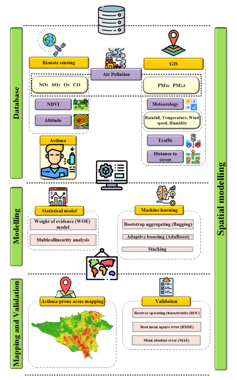
This research was conducted in five main steps (Figure 1). The materials (study area and data) and methods (machine learning methods, statistical methods, and validation methods) used in this research are described below.
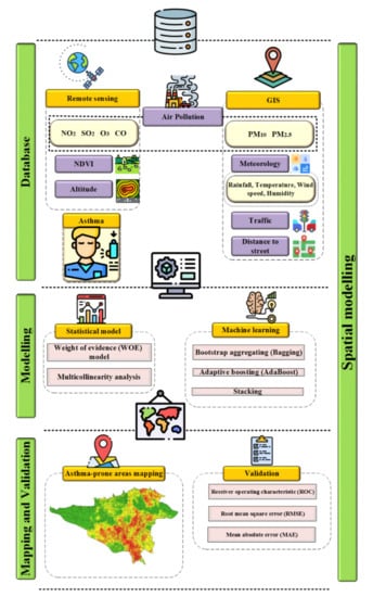
Figure 1.
Research methodologies.
2.1. Study Area
Tehran is Iran’s largest city and capital, as well as the center of the Tehran Province. It has a population of 8,244,535 and is the 25th most populous city in the world. The area of this city is 730 km2. Tehran is located in northern Iran, in the southern foothills of the Alborz Mountains, at a longitude of 51°2′E to 51°36′E, and a latitude of 35°34′N to 35°50′N. The height of the city in the highest points of the north reaches about 2000 m. Tehran’s climate is affected by mountains in the north and plains in the south. North of Tehran has a temperate and humid climate, and in other parts of the city is hot and dry and slightly cold in winter. The most important source of rainfall in Tehran is the humid Mediterranean and Atlantic winds that blow from the West. July and January are the hottest and coldest months of the year in Tehran, respectively. The maximum relative humidity is about 70% in the cold months and drops to 32% in the warm months. In Tehran, the highest rainfall occurs in winter with 43% of total rainfall and then in spring with 36%. The main land cover of Tehran includes residential (28.8%), streets (18.6%), and green space (11.4%). Among the problems of Tehran are heavy car traffic and air pollution, which affects respiratory disease (Figure 2).
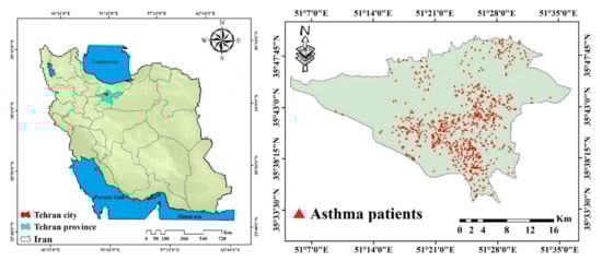
Figure 2.
Study area with asthma patients’ locations.
2.2. Asthma Data
The location of asthma patients was used as dependent data in the modeling of asthma disease. The locations of asthmatic patients in Tehran in 2019 were gathered using the information system of Tehran hospital. A total of 872 asthmatic patient locations were obtained, with 70% (611 locations) being used in modeling and 30% (261 locations) being used in the assessment. The holdout method was used to divide the training and test data (Figure 2).
2.3. Effective Criteria
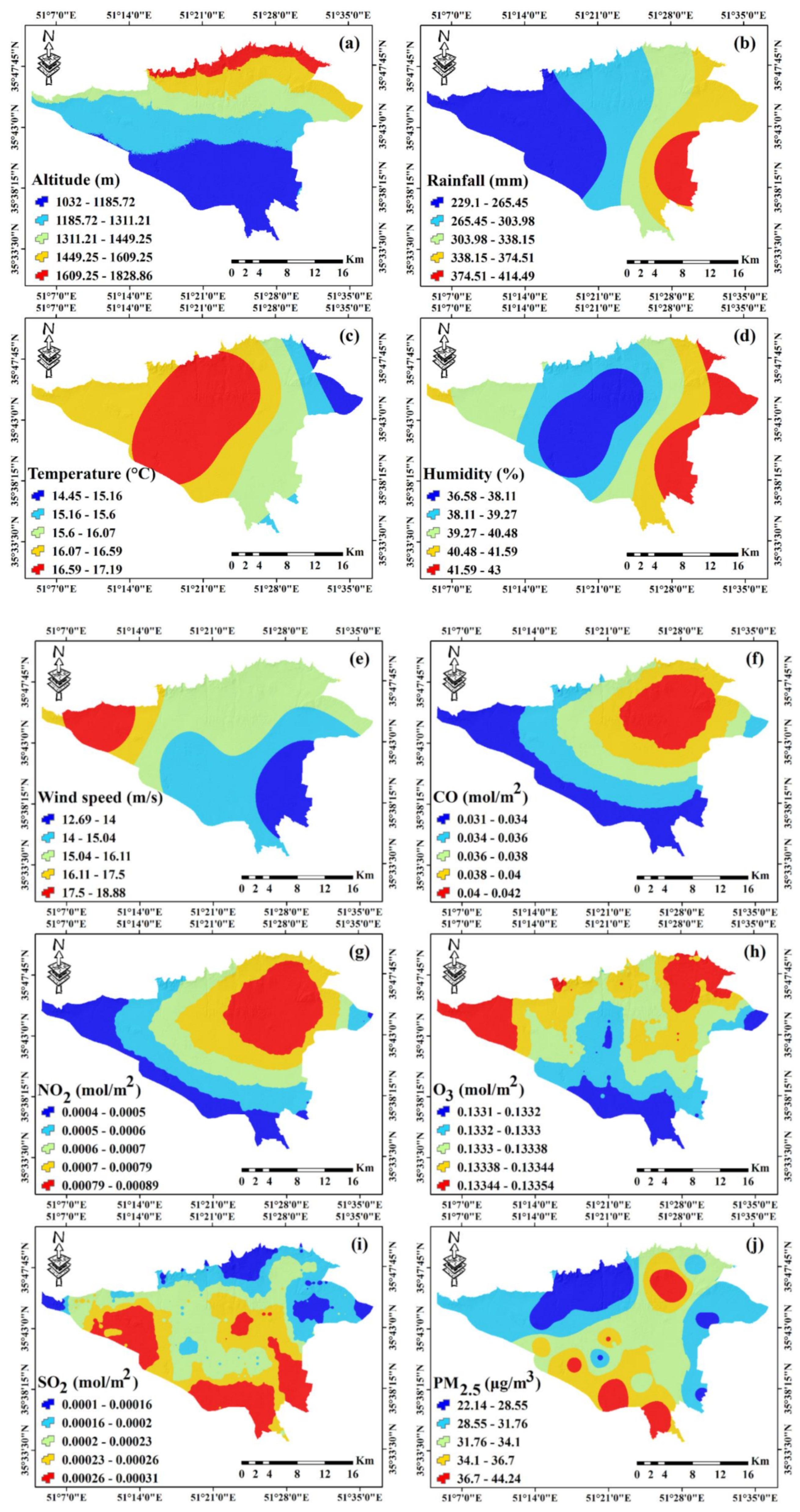
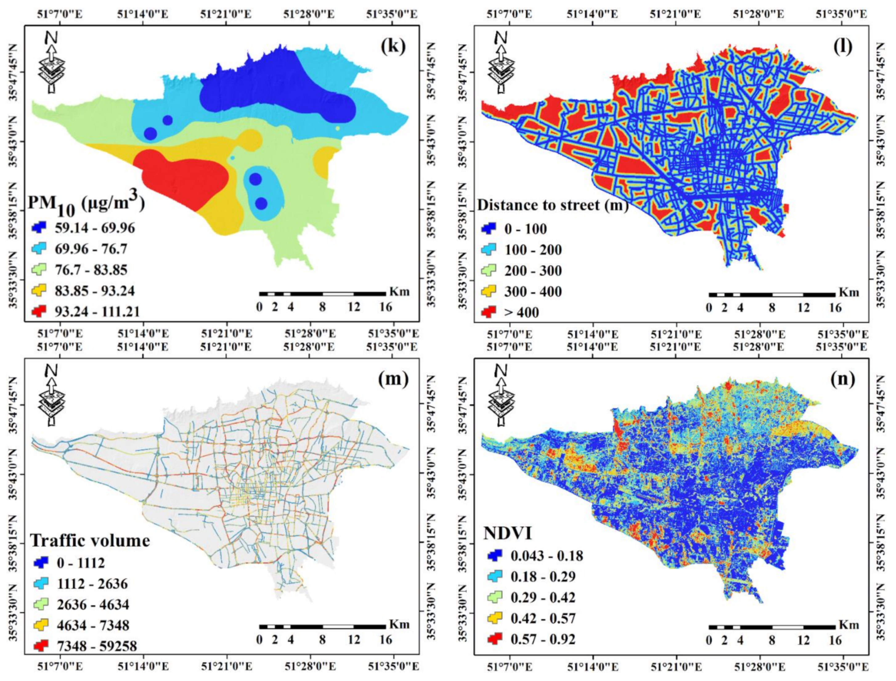
In this study, altitude, meteorology factors (rainfall, temperature, humidity, and wind speed), air pollutants (carbon monoxide (CO), Nitrogen dioxide (NO2), Ozone (O3), Sulfur dioxide (SO2), and particle matter (PM2.5 and PM10)), distance to the street, traffic volume, and NDVI were considered as factors affecting the occurrence of asthma (Figure 3). The spatial resolution of all effective factors was considered to be 30 × 30 m. Each of these factors is described below.

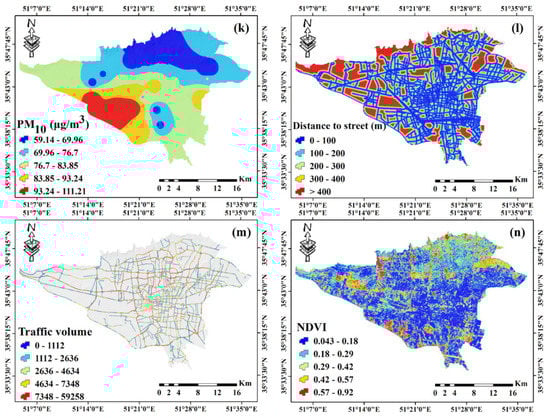
Figure 3.
Independent factor maps: (a) altitude, (b) rainfall, (c) temperature, (d) humidity, (e) wind speed, (f) CO, (g) NO2, (h) O3, (i) SO2, (j) PM2.5, (k) PM10, (l) distance to street, (m) traffic volume, and (n) NDVI.
- Altitude
Altitude can affect asthma by affecting oxygen levels, air pollutants, and climatic parameters [41]. A digital elevation model (DEM) was used to prepare the altitude map in 2019. Advanced space-borne thermal emission and reflection radiometer (ASTER) images with a pixel size of 30 m were used to create the DEM. Altitude layer processing and preparation for modeling were performed in ArcGIS 10.3 software.
- Meteorology data
Owing to the high impact of pollutants on the distribution and density of meteorological parameters, careful study of the relationship between air quality and weather conditions can help improve air pollution models to predict pollution crises, including its impact on human health such as lung diseases and asthma [42]. Therefore, in this study, meteorological parameters of rainfall, wind speed, temperature, and humidity were used from 2009 to 2019, and the annual average of these data were used to construct meteorological parameter maps for 12 meteorological stations in the Tehran province. The kriging interpolation technique in ArcGIS 10.3 software was used to prepare raster maps of meteorological parameters. Interpolation validation was carried by using Equations (1) and (2) (root mean square error (RMSE), and % RMSE). Because RMSE is sensitive to outlier data, % RMSE can be used instead. The lower the value of this index, the higher the accuracy of interpolation. The acceptable limit for % RMSE is <40, while values more than 70% indicate estimate point imprecision [43].
where is the average variable measured at each station, is the estimated predictor via kriging, and n is the total number of stations. Each measurement component average is represented by μ. The accuracy of interpolation of environmental factors is summarized in Table 1.

Table 1.
Result of interpolation accuracy.
The evaluation results of the kriging method showed acceptable accuracy for all meteorology factors (% RMSE < 40).
- Air pollutants
Toxic particles from air pollution can enter the lungs through the nose and cause variable damage to respiratory health. The prevalence of asthma and chronic pulmonary obstruction is directly related to increased air pollution [44]. Therefore, air pollutants are one of the factors affecting asthma. Sentinel 5P satellite imagery was used to prepare SO2, NO2, O3, and CO pollutants. The measurements’ spatial resolution (3.5 × 7 km2 for NO2, SO2, and O3, and 7 × 7 km2 for CO) allows air pollution observations. The average maps of these four pollutants were prepared for the time mentioned (July 2018 to December 2019) in the Google Earth Engine (GEE) platform and transferred to ArcGIS 10.3 software for further processing. Owing to the impossibility of direct monitoring of PM10 and PM2.5 pollutants by satellite images, station data were used to map these two pollutants. From 2009 to 2019, an average of air pollution data (PM10 and PM2.5) was collected from 23 air pollution monitoring stations in Tehran. In ArcGIS 10.3, the Kriging interpolation technique was employed to map these two pollutant parameters. The results of the interpolation evaluation of air pollution factors (Table 1) revealed that these factors were prepared with acceptable accuracy (% RMSE < 40).
- Distance to street
Streets are effective in creating traffic and air pollution. Street data were obtained from the open street map (OSM) at a scale of 1:100, 1000 in 2019. This criterion was prepared in ArcGIS 10.3 software using the Euclidean distance tool.
- Traffic volume
Vehicle fuel combustion gases are one of the most important air pollutants. Therefore, traffic plays an essential role in air pollution. This research used traffic volume to analyze the traffic impact on asthma [45]. Traffic volume is the number of vehicles that cross a road in one or more lanes at a given time. The traffic volume layer was created using the average annual traffic volume from 2015 to 2019. These data were collected from Tehran Traffic Control Company and processed in ArcGIS 10.3 software.
- Normalized difference vegetation index (NDVI)
By absorbing lead, dust, and soot from the air, green space helps to clean it up [46]. Therefore, green space can play an influential role in reducing air pollutants. The NDVI is a suitable method for calculating vegetation cover from satellite images and measuring vegetation volume [47]. The NDVI map was created using Landsat 7 images and the enhanced thematic mapper plus (ETM+) sensor. To create the NDVI map, the 2009–2019 annual average was used in the GEE platform. The scan line corrector (SLC) and the gap in Landsat images were corrected using a focal median filter. The NDVI index is calculated using Equation (3).
where denotes near-infrared reflectance (band 4—Landsat 7), and indicates red reflectance (band 3—Landsat 7). NDVI map with 30 m pixel size was prepared and transferred to ArcGIS 10.3 software for processing.
2.4. Factors Importance Using Gini Index
Breiman presented the Gini index, a divergence-based attribute splitting approach commonly used in the random forest (RF) algorithms [48]. When a variable is randomly selected, the Gini index measures the probability of it being incorrectly labeled [49]. The Gini index is calculated using Equation (4):
where denotes the probability of an element.
2.5. Multicollinearity Analysis
Multicollinearity occurs when two or more independent factors are highly interdependent. The inflation variance index (VIF) assesses that the parameters affecting asthma are independent of each other and can participate in modeling. Multicollinearity analysis is appropriate, according to previous studies, if the VIF value is less than 5 [50].
2.6. Weight of Evidence (WOE) Model
The weight of evidence is a data-driven method known as one of the methods of Bayesian theory in the form of the linear logarithm. The WOE model is defined based on the positive () and negative () weights [51]. The weight of each factor of asthma occurrence (A) dependent on the presence or absence of asthma locations (B) in the study area is as follows in this model (Equations (5) and (6)).
A positive weight () indicates a positive relationship between the presence of an influential factor, and a negative weight () indicates that the level of the relationship is negative. and show the presence and absence of asthma factors, respectively. and indicate the presence and absence of asthma, respectively. The difference between positive and negative weight is parameter (Equation (7)) [52]. The standard deviation of is determined by Equation (8):
where is the variance of and is the variance of. Weight variances are calculated as follows (Equations (9) and (10)):
The final weight of each category is calculated using Equation (11):
2.7. Bagging Algorithm
Breiman developed the bagging algorithm in 1996 to increase the classification and generalization of data [53]. This algorithm consists of a group of tree-based classifiers. This algorithm is a meta-algorithm based on the concepts of bootstrapping and combination to improve machine learning. Ensemble machine learning algorithms combine several weak learners to achieve a strong learner [54]. Bagging also helps to reduce variance and avoid over fitting. Bagging can be applied to any model, but decision trees are the most common. Bagging is a particular model of the average trend. In bagging, different training subsets are randomly selected by replacing all the training data. These individual predictors are combined using a method of averaging their decisions. For a test sample, the prediction value will be equal to the value obtained by averaging all predictors [55].
2.8. AdaBoost Algorithm
Freund and Schapire [56] proposed AdaBoost, an iterative algorithm for building a “powerful” classifier as a linear combination classification. Boosting is an ensemble meta-algorithm in machine learning used to reduce imbalances and variances. This method is based on combining the results of different categories to transform weak learning methods into strong ones [57]. A series of decision trees are created using the boosting method, with each tree attempting to reduce the error rate of incorrect classification. Then, each tree makes a prediction, and from these predictions, a vote is derived. Finally, a prediction with the highest number of options is selected as the final prediction [58].
2.9. Stacking Algorithm
The Stacking algorithm was developed in 1992 by Wolpert [59]. Stacking uses heterogeneous-based learning algorithms to implement ensemble learning. The Stacking algorithm structure consists of two levels: base-learners (level-0) and meta-learners (level-1). Meta-learners generalize the predictions of several base-learners by using the low-level output as the high-level input for relearning [60]. The three stages of the stacking algorithm are as follows: (1) by K-fold cross-validation, train various base classifiers using the training set; (2) to create a new reorganized training data set, gather the output predictions of these base classifiers; (3) train the meta-classifier with the new training data set. The stacking algorithm uses meta-learning steps to reduce estimation residuals [61].
2.10. Validation Metrics
- Receiver operating characteristic (ROC) curve
The ROC curve is one of the most important criteria for evaluating the performance of classified or multilayer models. This curve can measure models at different thresholds, and this curve is based on probability [62]. The TPR (True Positive Rate) is on the Y-axis, and the FPR (False Positive Rate) is on the X-axis in the ROC curve [63]. Based on a set threshold value such as T, a sample is considered positive if X > T and negative if X ≤ T. The random variable x here has a probability density function of for the time it is in the positive group; otherwise, its probability density function is specified by [64]. Therefore, TPR and FPR are calculated using Equations (12) and (13), respectively.
The best model is one in which the area under the curve (AUC) is close to one. This means that the closer to one, the more accurate and appropriate the measurement [65].
- Prediction error metrics
The performance of prediction models was assessed using the RMSE and mean absolute error (MAE) indices [66]. The MAE index was calculated using Equation (14):
where is the calculated value of the model, is the value of the observational variables, and n is the number of observations.
3. Results
3.1. Result of Multicollinearity Analysis
Table 2 shows the results of the multicollinearity analysis. The VIF value for all independent variables was less than five, according to the findings. It indicates that there was no multicollinearity in the independent factors used. As a result, modeling should include all independent variables.
Table 2.
Result of multicollinearity analysis.
3.2. Result of Gini Index
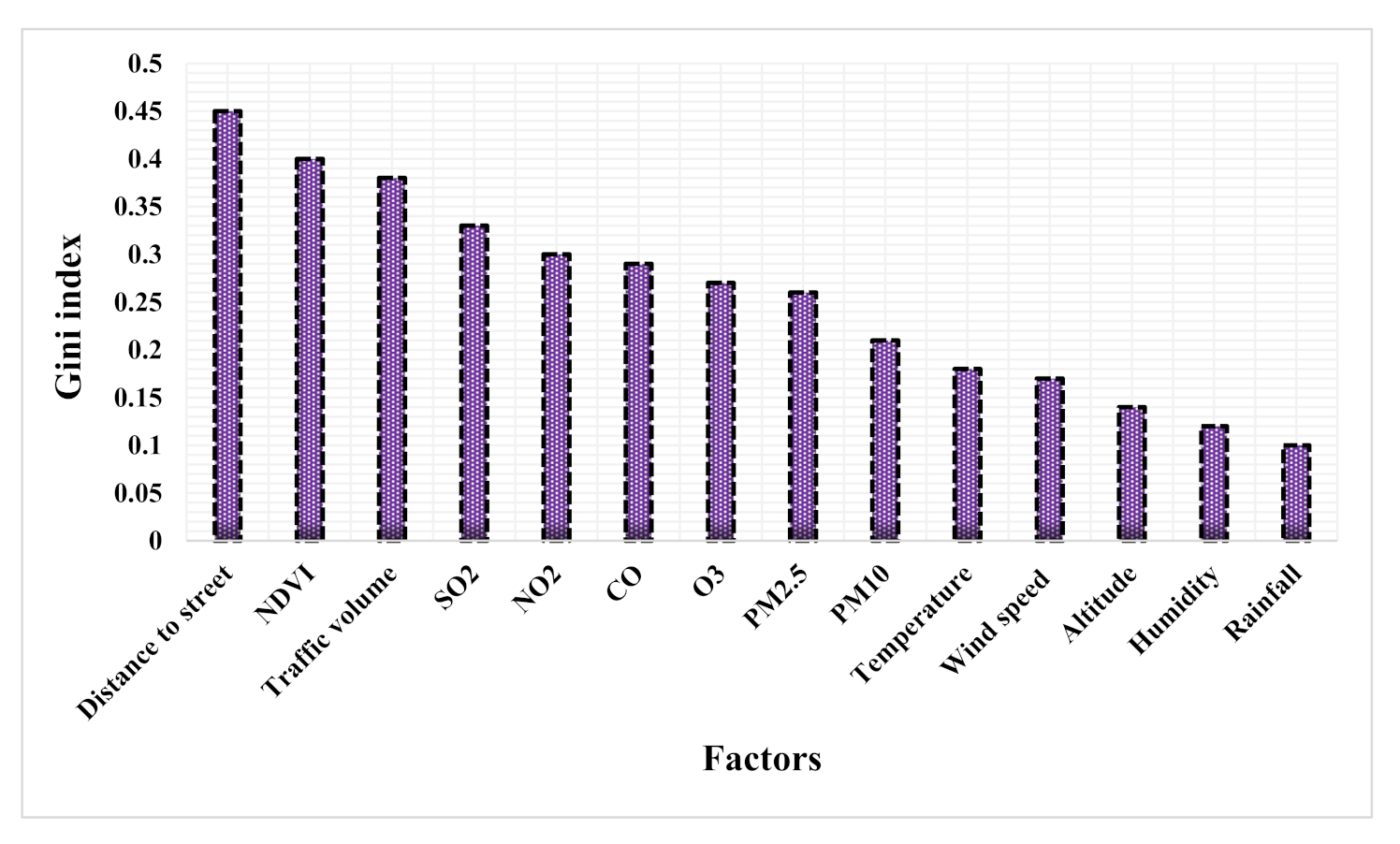
Figure 4 shows the importance of effective factors in modeling with the Gini index. According to the results, the distance to the street (0.45), NDVI (0.4), traffic volume (0.38), SO2 (0.33), NO2 (0.3), CO (0.29), O3 (0.27), PM2.5 (0.26), PM10 (0.21), temperature (0.18), wind speed (0.17), altitude (0.14), humidity (0.12), and rainfall (0.1) are the most important in modeling, respectively.

Figure 4.
Result of Gini index.
3.3. Result of WOE Model
Table 3 shows the results of the relationship between independent and dependent variables using the WOE model. In the altitude criterion, the highest weight belongs to class 1032–1185.72. According to the rainfall results, asthma occurrence rises initially with rising rainfall, then declines with high rainfall. The results of the temperature criterion show that the class 15.6–16.07 has the highest weight (WOE value = 6.7). In the humidity, the highest incidence of asthma occurs at high humidity (40.48%–41.59%). Asthma is more likely to arise at lower wind speeds. Class 14–15.04 m/s has the highest weight in the wind speed factor (WOE value = 12.01). The results of the CO factor show that as the levels of this pollutant increase, the probability of asthma increases. However, most of the weight of this criterion is related to the middle classes (WOE value = 3.98). The highest weight of the WOE model (WOE value = 4.08) for the NO2 factor occurs at high values of this parameter. Factor O3 is inversely related to the occurrence of asthma in the study area. As a result, asthma is more prone to be created in small concentrations of this pollutant. The results of the SO2 factor show that the highest weight is related to high levels of this pollutant (WOE value = 6.97). According to PM2.5, the highest weight belongs to the class 31.76–34.1 (WOE value = 11.26). The highest weight of the PM10 factor is in the 76.7–83.85 class (WOE value = 3.73). At distances close to the street, the highest incidence of asthma occurs, so the highest weight (WOE value = 4.7) is related to the class of 100–200 m. The spatial relationship between the occurrence of asthma and the volume of traffic shows the probability of asthma occurring in high amounts of this factor (WOE value = 8.13). The results of the NDVI factor reveal that asthma is more likely to occur with lower values of this parameter (0.043–0.18).
Table 3.
Result of WOE model.
3.4. Result of Modeling and Mapping
For modeling, a spatial database containing asthma data and influencing factors were built. In addition to occurrence data (value 1), we require nonoccurrence data (value 0) for improved network training in machine learning models. Nonoccurrence data were collected at random in the study area, much like the number of occurrence data. Therefore, spatial databases including dependent data (872 asthma occurrence locations and 872 non-asthma occurrence locations) and independent data (WOE model weight for factors) were considered modeling input. Seventy percent of the database was used as training data and 30% as validation data. The Waikato Environment for Knowledge Analysis (WEKA) software was used to implement the three ensemble algorithms. The parameters used in each algorithm are shown in Table 4.
Table 4.
Parameters used by ensemble algorithms.
After training the three algorithms, RMSE and MAE indices were used to evaluate the accuracy of the algorithms. The results of the RMSE and MAE indices are presented in Table 5. Based on the results, the RMSE index values for training and validation data are for AdaBoost (0.1678, 0.252), Bagging (0.2169, 0.3241), and Stacking (0.2353, 0.3488) algorithms, respectively. According to the results, the AdaBoost (0.0572, 0.2049), Bagging (0.1531, 0.2773), and Stacking (0.1555, 0.3073) algorithms have the highest accuracy based on MAE index values for training and validation data, respectively. The graph of the error rate between the predicted values and the actual data for each algorithm for training and test data is shown in Figure 5. The results show that algorithms AdaBoost, Bagging, and Stacking have the highest accuracy in modeling asthma-prone areas, respectively.
Table 5.
Result of metrics indices.
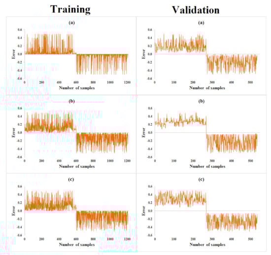
Figure 5.
Results of prediction error by: (a) AdaBoost, (b) Bagging, and (c) Stacking.
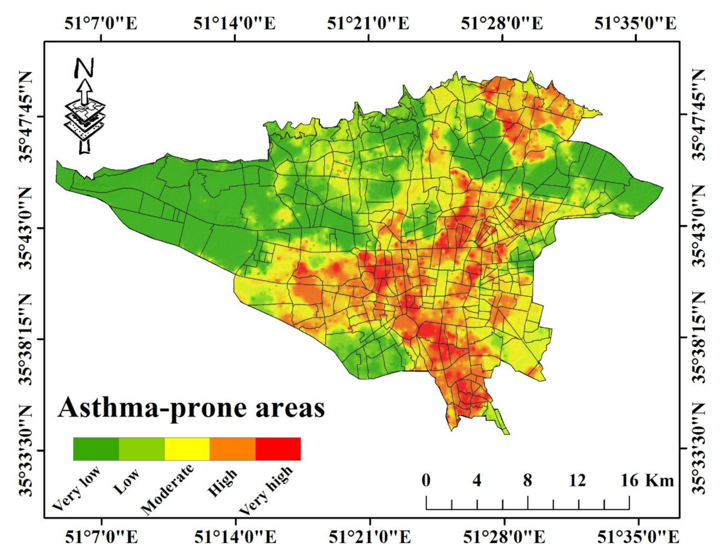
After training the three algorithms, the fitted model for each algorithm was generalized to the whole study area. The output of the three algorithms were converted from WEKA software to ArcGIS 10.3 and were used for asthma-prone area mapping. The spatial mapping of the asthma was divided into five classes based on the natural breaks classification method: very low, low, moderate, high, and very high. The asthma-prone areas mapping using AdaBoost algorithm is shown in Figure 6.

Figure 6.
Asthma-prone areas map by the AdaBoost algorithm.
3.5. Result of Validation
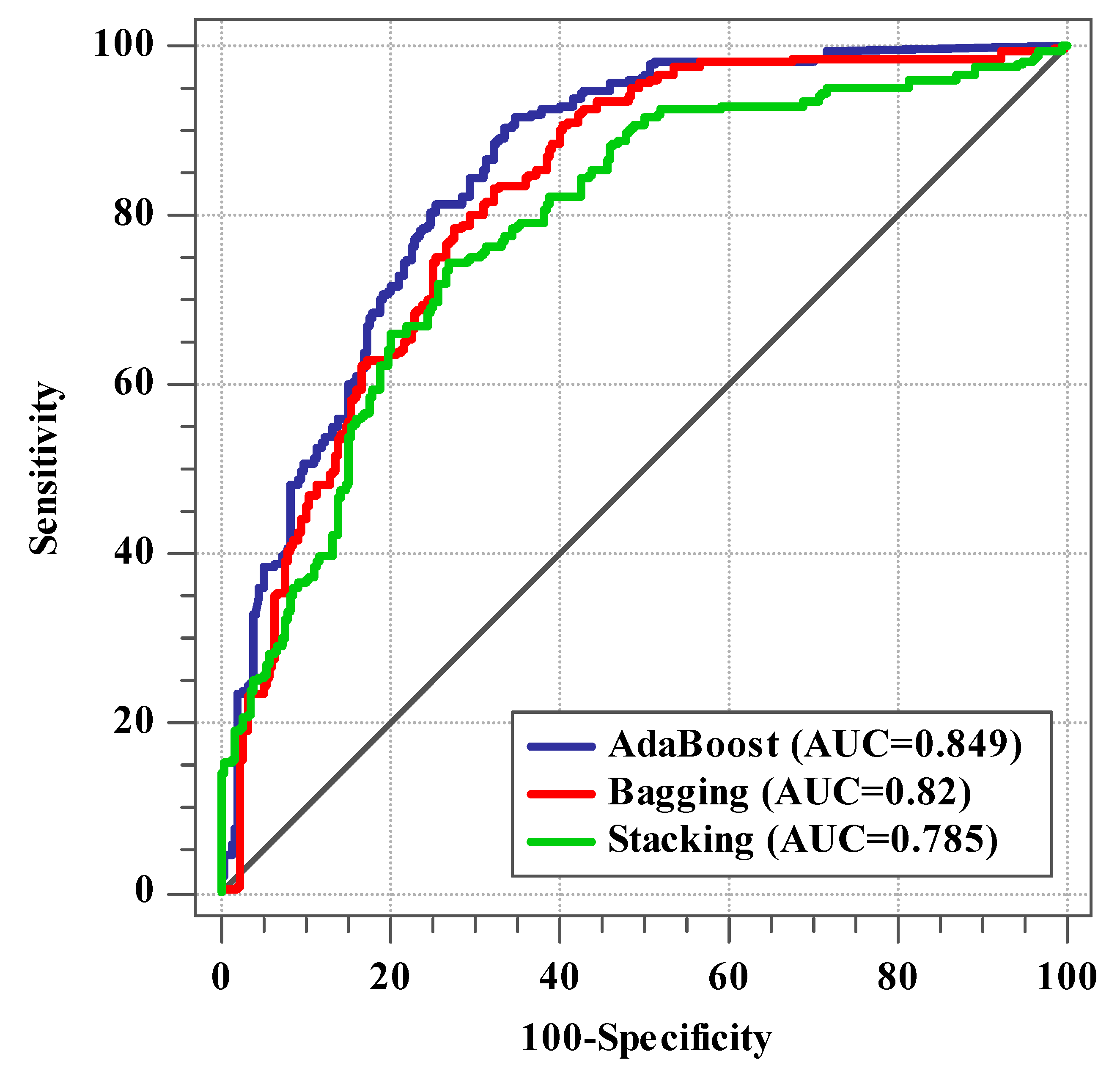
Thirty percent of the data on asthma occurrence and nonoccurrence were used to test the map of asthma-prone areas. The ROC curve and AUC in MedCalc software were used for validation. The results of the validation with the ROC curve are shown in Figure 7. The AUC values for AdaBoost, Bagging, and Stacking algorithms are 0.849, 0.82, and 0.785, respectively. The results show that the AdaBoost algorithm is more accurate than the other two algorithms in modeling asthma-prone areas. The results showed good accuracy of AdaBoost and Bagging algorithms and relatively good accuracy of the Stacking algorithm in modeling asthma-prone areas.
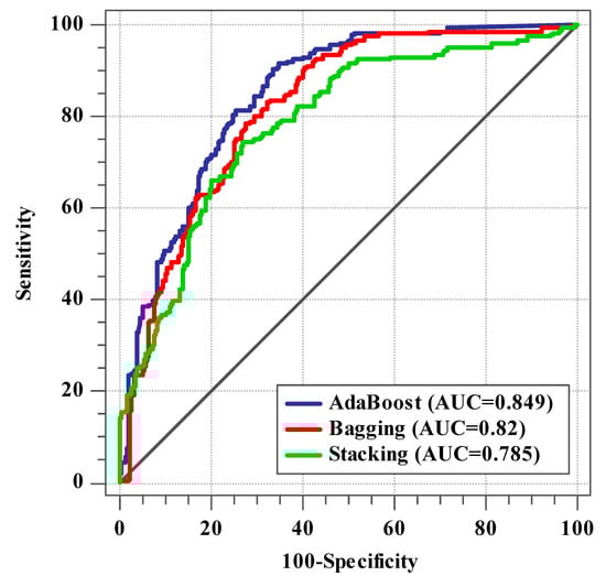
Figure 7.
ROC curve results by three algorithms.
According to the AdaBoost algorithm, 16.83% of the area is situated in the very high class, 19.1% in high, 18.5% in moderate, 13.82% in low, and 31.75% in the very low class. The Bagging algorithm assigns 19.22, 21.12, 17.4, 23.99, and 18.27% to the very high, high, moderate, low, and very low categories, respectively. For the Stacking algorithm, similar classes are 17.81, 20.35, 18.43, 27.54, and 15.87%.
4. Discussion
As there is no cure for asthma, it might be helpful to analyze the environmental factors that influence the incidence of this disease to prevent and manage it. Therefore, the aim of this study was spatial modeling of asthma-prone areas with ensemble machine learning algorithms. The WOE model was used to investigate the spatial relationship between independent and dependent data and the input of machine learning algorithms. The WOE model is a useful tool for dealing with nonlinearities between predictor and target [67]. According to the results of the WOE model, lower altitude values had a greater effect on the occurrence of asthma. Low-level pollution, such as that generated by transportation, generally decreases with altitude. This implies that areas will mostly hang suspended mid-air or build up into dense clouds at lower altitudes [68]. Rainfall results showed that at low and high levels of this factor, the probability of asthma is low. Rainfall can have a variety of effects on people with asthma. Pollen may be washed away by light rain, which may help with asthma symptoms. However, heavy rain can scatter pollen quickly into the air. On the other hand, heavy rainfall reduces air pollutants [69]. Owing to the different effects of rainfall, a moderate amount of rainfall can help reduce asthma [70]. Temperature factors, such as rainfall factor, has a different effect on the occurrence of asthma. Cold air can dry out the tissues of the airways and cause them to become more sensitive and closed [71]. When the air temperature is cooler, exhaust pollutants may become trapped at the surface under a layer of dense, cold air [72]. Warm air rises throughout the summer months, dispersing contaminants from the Earth’s surface into the upper troposphere, while more sunlight causes O3 to form [73]. In this study, moderate values of temperature (15 °C) have a greater effect on the occurrence of asthma. The results of humidity analysis showed that higher values of this factor increase the risk of asthma. High humidity increases pollutants in the air. The O3 pollutant rises when humidity rises [74]. Asthma is more likely to arise with lower amounts of wind speed, according to the results. Because winds carry pollutants around, wind patterns influence air quality. High values of wind speed play an effective role in reducing air pollutants [75]. According to the results of the WOE model, increasing the CO factor reduces the incidence of asthma. In this study, CO did not play its role well in modeling asthma-prone areas. The results of SO2 showed that higher values of this factor are more likely to cause asthma. Sulfur oxides, in combination with suspended particles and moisture, increases air pollution. The most common source of SO2 is fossil fuel combustion [76]. In this research, increasing the amount of NO2 pollutants increases the risk of asthma. The consumption of fuels at higher temperatures in refineries, petrochemicals, power plants, and household and commercial heating systems are all sources of NO2 [77]. The results of the O3 factor showed that this factor has no positive effect on the occurrence of asthma in the study area. O3 factor occurs more in summer and has less effect on increasing air pollution in cold seasons. As a result, asthma appears to be more common in Tehran during the cold seasons, while O3 pollution appears to have minimal influence on the prevalence of asthma throughout these seasons [36]. The findings of PM2.5 and PM10 revealed that as these factor values rise, the probability of asthma in the study area rises. Combustion processes produce a major portion of the PM in urban air. The size of airborne particles affects the respiratory system, and as the particle size decreases, the symptoms increase more severely [78]. Based on the results of the Gini index in air pollutants, SO2, NO2, CO, O3, PM2.5, and PM10 factors are the most important in modeling, respectively. The results of this study are not consistent with Razavi-Termeh et al.’s [7] research. In a study conducted by Razavi-Termeh et al. [7], all air pollutants were prepared based on ground station data, and PM2.5 and PM10 factors were the most important in modeling. However, in this research, because of the use of remote sensing images to produce air pollutants (SO2, NO2, CO, and O3), the SO2 factor is the most important. This method has the advantage of allowing for more accurate air quality measurements in urban areas with few monitoring stations [79]. The distance to the street factor indicates that shorter distances are more likely to induce asthma. Additionally, at higher levels of traffic volume factor, asthma is more likely to occur. According to the Gini index, these two factors were significantly relevant in the occurrence of asthma. In the distances close to the street, due to the traffic of cars, the air pollution is higher and also the high traffic causes more stopping of the cars and increasing the emission of air pollutants [80]. The results of the NDVI factor showed that in smaller amounts of this factor, asthma is more likely to occur. Additionally, according to the Gini index, this factor is of great importance in modeling asthma-prone areas. The concentrations of air pollutants were comparatively low in areas with high NDVI. Because vegetation has a dust-blocking effect, places with less vegetation are more likely to create particulate matter [81]. In urban environments, high population density causes more traffic, less green space and thus increases air pollution [43]. Therefore, living in densely populated areas causes infectious rhinitis, respiratory infections, and asthma [82].
AdaBoost, Bagging, and Stacking algorithms, respectively, had the highest accuracy in predicting asthma-prone areas, according to the findings of assessment indicators. The AdaBoost algorithm was more capable of modeling asthma-prone areas in the study area than the other two algorithms. Advantages of the AdaBoost algorithm over two algorithms is [83]: (1) the ability to merge different types of predictors; (2) decreases bias; (3) models are weighed in Boosting according to their performance; (4) when dealing with bias or under fitting in a data set, the boosting approach comes in useful. The Bagging algorithm has higher accuracy than the stacking algorithm owing to reducing the variance and solving the over fitting problem [84]. Because the Stacking algorithm does not use sampling in the training dataset and does not use a sequence of models to correct the predictions of prior models, it is less accurate than the other two algorithms [85].
The innovations of the present study including, the use of remote sensing to prepare criteria affecting the occurrence of asthma, the use of the WOE statistical method to determine the spatial relationship between independent and dependent criteria, and the use of ensemble machine learning algorithms to map asthma-prone areas. The limitations of the present study included the lack of access to up-to-date population density data, and the lack of direct access to PM2.5 and PM10 pollutant data using remote sensing images. For future research, it is suggested that PM2.5 and PM10 pollutants and climatic parameters be prepared using remote sensing images.
5. Conclusions
A combination of GIS, RS, and ensemble machine learning algorithms were employed in this work to propose a strategy for the prevention and management of asthma in urban areas. The results showed that the ensemble machine learning algorithms have good accuracy in modeling asthma-prone areas, where the AdaBoost algorithm showed higher accuracy than the other two algorithms. Low altitude, high rainfall and humidity, moderate temperature, low wind speed, high levels of air pollutants (except O3), shorter street distance, high traffic volume, and less vegetation all played a part in the prevalence of asthma in Tehran, according to the results of the WOE model. Factors including distance to the street, traffic volume, and NDVI were all important in modeling. Less distance from the street, high traffic volume, and less vegetation increase the emission of pollutants. It seems that air pollution is the primary cause of asthma attacks in Tehran. Remote sensing factors such as NDVI and four air pollutants (SO2, NO2, CO, and O3) played an essential role in modeling asthma-prone areas. Remote sensing factors such as NDVI and four air pollutants played an essential role in modeling asthma-prone areas. Remote sensing images have an excellent ability to integrate with GIS in spatial modeling of diseases owing to the monitoring of environmental factors anywhere in the world at any time. The center and southern parts of Tehran are more in danger, according to asthma risk maps. These regions have a significant impact on increasing levels of air pollution due to their high population density and transportation. Community planners and administrators will be aided using maps of asthma-prone regions for the management and presentation of asthma.
Author Contributions
Conceptualization, S.V.R.-T. and A.S.-N.; data creation, S.V.R.-T.; formal analysis, S.V.R.-T.; funding acquisition, S.-M.C.; investigation, S.V.R.-T.; methodology, S.V.R.-T.; project administration, S.-M.C.; resources, A.S.-N.; software, S.V.R.-T.; supervision, A.S.-N.; validation, S.V.R.-T.; visualization, S.V.R.-T.; writing—original draft, S.V.R.-T.; writing—review and editing, A.S.-N. and S.-M.C. All authors have read and agreed to the published version of the manuscript.
Funding
This research was supported by MSIT (Ministry of Science and ICT), Korea, under the ITRC (Information Technology Research Center) support program (IITP-2021-2016-0-00312) supervised by the IITP (Institute for Information and Communications Technology Planning and Evaluation).
Institutional Review Board Statement
Not applicable.
Informed Consent Statement
Not applicable.
Data Availability Statement
Data during the current study are not publicly available due to integrity and legal reasons but are available from the corresponding author on reasonable request.
Conflicts of Interest
The authors declare no conflict of interest.
References
- Ehteshami-Afshar, S.; FitzGerald, J.; Doyle-Waters, M.; Sadatsafavi, M. The global economic burden of asthma and chronic obstructive pulmonary disease. Int. J. Tuberc. Lung Dis. 2016, 20, 11–23. [Google Scholar] [CrossRef]
- Nunes, C.; Pereira, A.M.; Morais-Almeida, M. Asthma costs and social impact. Asthma Res. Pract. 2017, 3, 1–11. [Google Scholar] [CrossRef] [Green Version]
- Lundbäck, B.; Backman, H.; Lötvall, J.; Rönmark, E. Is asthma prevalence still increasing? Expert Rev. Respir. Med. 2016, 10, 39–51. [Google Scholar] [CrossRef] [PubMed]
- Ma, R.; Liang, L.; Kong, Y.; Zhai, S.; Gu, J.; Zhang, G.; Wang, T. Hotspot detection and socio-ecological factor analysis of asthma hospitalization rate in guangxi, china. Environ. Res. 2020, 183, 109201. [Google Scholar] [CrossRef] [PubMed]
- Becker, A.B.; Abrams, E.M. Asthma guidelines: The global initiative for asthma in relation to national guidelines. Curr. Opin. Allergy Clin. Immunol. 2017, 17, 99–103. [Google Scholar] [CrossRef]
- Žavbi, M.; Korošec, P.; Fležar, M.; Kristan, S.Š.; Malovrh, M.M.; Rijavec, M. Polymorphisms and haplotypes of the chromosome locus 17q12-17q21. 1 contribute to adult asthma susceptibility in slovenian patients. Hum. Immunol. 2016, 77, 527–534. [Google Scholar] [CrossRef]
- Razavi-Termeh, S.V.; Sadeghi-Niaraki, A.; Choi, S.-M. Asthma-prone areas modeling using a machine learning model. Sci. Rep. 2021, 11, 1–16. [Google Scholar] [CrossRef]
- Dias, C.S.; Dias, M.A.S.; Friche, A.A.d.L.; Almeida, M.C.d.M.; Viana, T.C.; Mingoti, S.A.; Caiaffa, W.T. Temporal and spatial trends in childhood asthma-related hospitalizations in belo horizonte, minas gerais, brazil and their association with social vulnerability. Int. J. Environ. Res. Public Health 2016, 13, 704. [Google Scholar] [CrossRef] [Green Version]
- Kabesch, M. Gene by environment interactions and the development of asthma and allergy. Toxicol. Lett. 2006, 162, 43–48. [Google Scholar] [CrossRef]
- Khan, I.A.; Arsalan, M.H.; Mehdi, M.R.; Kazmi, J.H.; Seong, J.C.; Han, D. Assessment of asthma-prone environment in karachi, pakistan using gis modeling. JPMA J. Pak. Med Assoc. 2020, 70, 636–649. [Google Scholar] [CrossRef]
- Portnov, B.A.; Reiser, B.; Karkabi, K.; Cohen-Kastel, O.; Dubnov, J. High prevalence of childhood asthma in northern israel is linked to air pollution by particulate matter: Evidence from gis analysis and bayesian model averaging. Int. J. Environ. health Res. 2012, 22, 249–269. [Google Scholar] [CrossRef]
- Svendsen, E.R.; Gonzales, M.; Mukerjee, S.; Smith, L.; Ross, M.; Walsh, D.; Rhoney, S.; Andrews, G.; Ozkaynak, H.; Neas, L.M. Gis-modeled indicators of traffic-related air pollutants and adverse pulmonary health among children in el paso, texas. Am. J. Epidemiol. 2012, 176, S131–S141. [Google Scholar] [CrossRef] [Green Version]
- Lee, S.-J.; Yeatts, K.B.; Serre, M.L. A bayesian maximum entropy approach to address the change of support problem in the spatial analysis of childhood asthma prevalence across north carolina. Spat. Spatio-Temporal Epidemiol. 2009, 1, 49–60. [Google Scholar] [CrossRef] [PubMed] [Green Version]
- Jaya, I.G.N.M.; Folmer, H. Bayesian spatiotemporal mapping of relative dengue disease risk in bandung, indonesia. J. Geogr. Syst. 2020, 22, 105–142. [Google Scholar] [CrossRef]
- Mertikas, S.P.; Partsinevelos, P.; Mavrocordatos, C.; Maximenko, N.A. Environmental Applications of Remote Sensing. In Pollution Assessment for Sustainable Practices in Applied Sciences and Engineering; Elsevier: Amsterdam, The Netherlands, 2021; pp. 107–163. [Google Scholar]
- Dash, J.P.; Pearse, G.D.; Watt, M.S. Uav multispectral imagery can complement satellite data for monitoring forest health. Remote Sens. 2018, 10, 1216. [Google Scholar] [CrossRef] [Green Version]
- Beloconi, A.; Vounatsou, P. Bayesian geostatistical modelling of high-resolution no2 exposure in europe combining data from monitors, satellites and chemical transport models. Environ. Int. 2020, 138, 105578. [Google Scholar] [CrossRef]
- Yuniarti, E.; Hermon, D.; Dewata, I.; Barlian, E.; Iswamdi, U. Mapping the high risk populations against coronavirus disease 2019 in padang west sumatra indonesia. Int. J. Progress. Sci. Technol. 2020, 20, 50–58. [Google Scholar]
- Razavi-Termeh, S.V.; Sadeghi-Niaraki, A.; Choi, S.-M. Coronavirus disease vulnerability map using a geographic information system (gis) from 16 april to 16 may 2020. Phys. Chem. Earth Parts A/B/C 2021, 103043. [Google Scholar] [CrossRef]
- Gebre-Michael, T.; Malone, J.; Balkew, M.; Ali, A.; Berhe, N.; Hailu, A.; Herzi, A. Mapping the potential distribution of phlebotomus martini and p. Orientalis (diptera: Psychodidae), vectors of kala-azar in east africa by use of geographic information systems. Acta Tropica 2004, 90, 73–86. [Google Scholar] [CrossRef]
- BenBella, D.; Ghosh, D. Combining geospatial analysis with hiv care continuum to identify differential hiv/aids treatment indicators in uganda. Prof. Geogr. 2021, 73, 213–229. [Google Scholar] [CrossRef]
- Pham, N.T.; Nguyen, C.T.; Vu, H.H. Assessing and modelling vulnerability to dengue in the mekong delta of vietnam by geospatial and time-series approaches. Environ. Res. 2020, 186, 109545. [Google Scholar] [CrossRef]
- Jenila, V.M.; Varalakshmi, P.; Rajasekar, S.J.S. Geospatial Mapping, Epidemiological Modelling, Statistical Correlation and Analysis of Covid-19 with Forest Cover and Population in the Districts of Tamil Nadu, India. In Proceedings of the 2020 IEEE International Conference on Advent Trends in Multidisciplinary Research and Innovation (ICATMRI), Buldana, India, 3 December 2020; pp. 1–7. [Google Scholar]
- Abdullah, A.Y.M.; Dewan, A.; Shogib, M.R.I.; Rahman, M.M.; Hossain, M.F. Environmental factors associated with the distribution of visceral leishmaniasis in endemic areas of bangladesh: Modeling the ecological niche. Trop. Med. Health 2017, 45, 1–15. [Google Scholar] [CrossRef]
- Gordian, M.E.; Haneuse, S.; Wakefield, J. An investigation of the association between traffic exposure and the diagnosis of asthma in children. J. Expo. Sci. Environ. Epidemiol. 2006, 16, 49–55. [Google Scholar] [CrossRef] [PubMed]
- Gorai, A.K.; Tuluri, F.; Tchounwou, P.B. A gis based approach for assessing the association between air pollution and asthma in new york state, USA. Int. J. Environ. Res. Public Health 2014, 11, 4845–4869. [Google Scholar] [CrossRef] [Green Version]
- Samuels-Kalow, M.E.; Camargo, C.A. The use of geographic data to improve asthma care delivery and population health. Clin. chest Med. 2019, 40, 209–225. [Google Scholar] [CrossRef]
- Ouédraogo, A.M.; Crighton, E.J.; Sawada, M.; To, T.; Brand, K.; Lavigne, E. Exploration of the spatial patterns and determinants of asthma prevalence and health services use in ontario using a bayesian approach. PLoS ONE 2018, 13, e0208205. [Google Scholar] [CrossRef] [Green Version]
- Zook, M.; Wollersheim, D.; Erbas, B.; Jacobsen, K.H. Integrating spatial analysis into policy formulation: A case study examining traffic exposure and asthma. World Med Health Policy 2018, 10, 99–110. [Google Scholar] [CrossRef]
- Pala, D.; Pagán, J.; Parimbelli, E.; Rocca, M.T.; Bellazzi, R.; Casella, V. Spatial enablement to support environmental, demographic, socioeconomics, and health data integration and analysis for big cities: A case study with asthma hospitalizations in new york city. Front. Med. 2019, 6, 84. [Google Scholar] [CrossRef] [Green Version]
- Leynaert, B.; Le Moual, N.; Neukirch, C.; Siroux, V.; Varraso, R. Environmental risk factors for asthma developement. Presse Med. 2019, 48, 262–273. [Google Scholar] [CrossRef]
- Kinghorn, B.; Fretts, A.M.; O’Leary, R.A.; Karr, C.J.; Rosenfeld, M.; Best, L.G. Socioeconomic and environmental risk factors for pediatric asthma in an american indian community. Acad. Pediatrics 2019, 19, 631–637. [Google Scholar] [CrossRef]
- Krautenbacher, N.; Kabesch, M.; Horak, E.; Braun-Fahrländer, C.; Genuneit, J.; Boznanski, A.; von Mutius, E.; Theis, F.; Fuchs, C.; Ege, M.J. Asthma in farm children is more determined by genetic polymorphisms and in non-farm children by environmental factors. Pediatric Allergy Immunol. 2021, 32, 295–304. [Google Scholar] [CrossRef]
- Hauptman, M.; Gaffin, J.M.; Petty, C.R.; Sheehan, W.J.; Lai, P.S.; Coull, B.; Gold, D.R.; Phipatanakul, W. Proximity to major roadways and asthma symptoms in the school inner-city asthma study. J. Allergy Clin. Immunol. 2020, 145, 119–126.e114. [Google Scholar] [CrossRef] [PubMed] [Green Version]
- Rodríguez-Orozco, A.R.; Galeana-Osuna, E.G.; Bollo-Manent, M.; Figueroa-Núñez, B. Spatial analysis of asthma morbidity in the city of morelia, mexico, for the decade 2000–2010. Atencion Primaria 2020, 52, 578–579. [Google Scholar] [CrossRef]
- Razavi-Termeh, S.V.; Sadeghi-Niaraki, A.; Choi, S.-M. Effects of air pollution in spatio-temporal modeling of asthma-prone areas using a machine learning model. Environ. Res. 2021, 200, 111344. [Google Scholar] [CrossRef]
- Shinkuma, R.; Nishio, T. Data Assessment and Prioritization in Mobile Networks for Real-Time Prediction of Spatial Information with Machine Learning. In Proceedings of the 2019 IEEE First International Workshop on Network Meets Intelligent Computations (NMIC), Dallas, TX, USA, 7–9 July 2019; pp. 1–6. [Google Scholar]
- Shahhosseini, M.; Hu, G.; Pham, H. Optimizing ensemble weights and hyperparameters of machine learning models for regression problems. arXiv 2019, arXiv:1908.05287. [Google Scholar]
- Ribeiro, M.H.D.M.; dos Santos Coelho, L. Ensemble approach based on bagging, boosting and stacking for short-term prediction in agribusiness time series. Appl. Soft Comput. 2020, 86, 105837. [Google Scholar] [CrossRef]
- Wen, L.; Hughes, M. Coastal wetland mapping using ensemble learning algorithms: A comparative study of bagging, boosting and stacking techniques. Remote Sens. 2020, 12, 1683. [Google Scholar] [CrossRef]
- Giraldo-Cadavid, L.F.; Perdomo-Sanchez, K.; Córdoba-Gravini, J.L.; Escamilla, M.I.; Suarez, M.; Gelvez, N.; Gozal, D.; Duenas-Meza, E. Allergic rhinitis and osa in children residing at a high altitude. Chest 2020, 157, 384–393. [Google Scholar] [CrossRef]
- Delamater, P.L.; Finley, A.O.; Banerjee, S. An analysis of asthma hospitalizations, air pollution, and weather conditions in Los Angeles County, california. Sci. Total Environ. 2012, 425, 110–118. [Google Scholar] [CrossRef] [Green Version]
- Shogrkhodaei, S.Z.; Razavi-Termeh, S.V.; Fathnia, A. Spatio-temporal modeling of pm2. 5 risk mapping using three machine learning algorithms. Environ. Pollut. 2021, 289, 117859. [Google Scholar] [CrossRef]
- Schraufnagel, D.E.; Balmes, J.R.; Cowl, C.T.; De Matteis, S.; Jung, S.-H.; Mortimer, K.; Perez-Padilla, R.; Rice, M.B.; Riojas-Rodriguez, H.; Sood, A. Air pollution and noncommunicable diseases: A review by the forum of international respiratory societies’ environmental committee, part 2: Air pollution and organ systems. Chest 2019, 155, 417–426. [Google Scholar] [CrossRef] [PubMed]
- Tong, Z.; Li, Y.; Westerdahl, D.; Adamkiewicz, G.; Spengler, J.D. Exploring the effects of ventilation practices in mitigating in-vehicle exposure to traffic-related air pollutants in china. Environ. Int. 2019, 127, 773–784. [Google Scholar] [CrossRef] [PubMed]
- Cazorla, A.; Bahadur, R.; Suski, K.; Cahill, J.F.; Chand, D.; Schmid, B.; Ramanathan, V.; Prather, K. Relating aerosol absorption due to soot, organic carbon, and dust to emission sources determined from in-situ chemical measurements. Atmos. Chem. Phys. 2013, 13, 9337–9350. [Google Scholar] [CrossRef] [Green Version]
- Jamali, S.; Seaquist, J.; Eklundh, L.; Ardö, J. Automated mapping of vegetation trends with polynomials using ndvi imagery over the sahel. Remote Sens. Environ. 2014, 141, 79–89. [Google Scholar] [CrossRef]
- Liu, H.; Zhou, M.; Lu, X.S.; Yao, C. Weighted Gini Index Feature Selection Method for Imbalanced Data. In Proceedings of the 2018 IEEE 15th International Conference on Networking, Sensing and Control (ICNSC), Zhuhai, China, 27–29 March 2018; pp. 1–6. [Google Scholar]
- Tangirala, S. Evaluating the impact of gini index and information gain on classification using decision tree classifier algorithm. Int. J. Adv. Comput. Sci. Appl. 2020, 11, 612–619. [Google Scholar] [CrossRef]
- Olivoto, T.; de Souza, V.Q.; Nardino, M.; Carvalho, I.R.; Ferrari, M.; de Pelegrin, A.J.; Szareski, V.J.; Schmidt, D. Multicollinearity in path analysis: A simple method to reduce its effects. Agron. J. 2017, 109, 131–142. [Google Scholar] [CrossRef]
- Golbamaki, A.; Golbamaki, N.; Sizochenko, N.; Rasulev, B.; Leszczynski, J.; Benfenati, E. Genotoxicity induced by metal oxide nanoparticles: A weight of evidence study and effect of particle surface and electronic properties. Nanotoxicology 2018, 12, 1113–1129. [Google Scholar] [CrossRef]
- Hong, H.; Ilia, I.; Tsangaratos, P.; Chen, W.; Xu, C. A hybrid fuzzy weight of evidence method in landslide susceptibility analysis on the wuyuan area, china. Geomorphology 2017, 290, 1–16. [Google Scholar] [CrossRef]
- Breiman, L. Bagging predictors. Mach. Learn. 1996, 24, 123–140. [Google Scholar] [CrossRef] [Green Version]
- Galar, M.; Fernandez, A.; Barrenechea, E.; Bustince, H.; Herrera, F. A review on ensembles for the class imbalance problem: Bagging-, boosting-, and hybrid-based approaches. IEEE Trans. Syst. Man Cybern. Part C Appl. Rev. 2011, 42, 463–484. [Google Scholar] [CrossRef]
- Xia, T.; Zhuo, P.; Xiao, L.; Du, S.; Wang, D.; Xi, L. Multi-stage fault diagnosis framework for rolling bearing based on ohf elman adaboost-bagging algorithm. Neurocomputing 2021, 433, 237–251. [Google Scholar] [CrossRef]
- Freund, Y.; Schapire, R.E. A decision-theoretic generalization of on-line learning and an application to boosting. J. Comput. Syst. Sci. 1997, 55, 119–139. [Google Scholar] [CrossRef] [Green Version]
- Sultana, N.; Islam, M.M. Meta Classifier-Based Ensemble Learning for Sentiment Classification. In Proceedings of the International Joint Conference on Computational Intelligence, Budapest, Hungary, 2–4 November 2020; pp. 73–84. [Google Scholar]
- Dev, V.A.; Eden, M.R. Evaluating the Boosting Approach to Machine Learning for Formation Lithology Classification. In Computer Aided Chemical Engineering; Elsevier: Amsterdam, The Netherlands, 2018; Volume 44, pp. 1465–1470. [Google Scholar]
- Wolpert, D.H. Stacked generalization. Neural Netw. 1992, 5, 241–259. [Google Scholar] [CrossRef]
- Sesmero, M.P.; Ledezma, A.I.; Sanchis, A. Generating ensembles of heterogeneous classifiers using stacked generalization. Wiley Interdiscip. Rev. Data Min. Knowl. Discov. 2015, 5, 21–34. [Google Scholar] [CrossRef]
- Ghalejoogh, G.S.; Kordy, H.M.; Ebrahimi, F. A hierarchical structure based on stacking approach for skin lesion classification. Expert Syst. Appl. 2020, 145, 113127. [Google Scholar] [CrossRef]
- Farhangi, F.; Sadeghi-Niaraki, A.; Nahvi, A.; Razavi-Termeh, S.V. Spatial modeling of accidents risk caused by driver drowsiness with data mining algorithms. Geocarto Int. 2020, 1–15. [Google Scholar] [CrossRef]
- Ranjgar, B.; Razavi-Termeh, S.V.; Foroughnia, F.; Sadeghi-Niaraki, A.; Perissin, D. Land subsidence susceptibility mapping using persistent scatterer sar interferometry technique and optimized hybrid machine learning algorithms. Remote Sens. 2021, 13, 1326. [Google Scholar] [CrossRef]
- Hajian-Tilaki, K. Receiver operating characteristic (roc) curve analysis for medical diagnostic test evaluation. Casp. J. Intern. Med. 2013, 4, 627. [Google Scholar]
- Razavi-Termeh, S.V.; Khosravi, K.; Sadeghi-Niaraki, A.; Choi, S.-M.; Singh, V.P. Improving groundwater potential mapping using metaheuristic approaches. Hydrol. Sci. J. 2020, 65, 2729–2749. [Google Scholar] [CrossRef]
- Razavi-Termeh, S.V.; Sadeghi-Niaraki, A.; Choi, S.-M. Ubiquitous gis-based forest fire susceptibility mapping using artificial intelligence methods. Remote Sens. 2020, 12, 1689. [Google Scholar] [CrossRef]
- Rhomberg, L.R.; Bailey, L.A.; Goodman, J.E. Hypothesis-based weight of evidence: A tool for evaluating and communicating uncertainties and inconsistencies in the large body of evidence in proposing a carcinogenic mode of action—naphthalene as an example. Crit. Rev. Toxicol. 2010, 40, 671–696. [Google Scholar] [CrossRef] [PubMed]
- Sun, J.; Wang, Y.; Wu, F.; Tang, G.; Wang, L.; Wang, Y.; Yang, Y. Vertical characteristics of vocs in the lower troposphere over the north china plain during pollution periods. Environ. Pollut. 2018, 236, 907–915. [Google Scholar] [CrossRef] [PubMed]
- Shukla, J.; Misra, A.; Sundar, S.; Naresh, R. Effect of rain on removal of a gaseous pollutant and two different particulate matters from the atmosphere of a city. Math. Comput. Model. 2008, 48, 832–844. [Google Scholar] [CrossRef]
- Ho, W.-C.; Hartley, W.R.; Myers, L.; Lin, M.-H.; Lin, Y.-S.; Lien, C.-H.; Lin, R.-S. Air pollution, weather, and associated risk factors related to asthma prevalence and attack rate. Environ. Res. 2007, 104, 402–409. [Google Scholar] [CrossRef]
- Kaminsky, D.A.; Bates, J.H.; Irvin, C.G. Effects of cool, dry air stimulation on peripheral lung mechanics in asthma. Am. J. Respir. Crit. Care Med. 2000, 162, 179–186. [Google Scholar] [CrossRef]
- Zhang, W.; Zhang, Y.; Gong, J.; Yang, B.; Zhang, Z.; Wang, B.; Zhu, C.; Shi, J.; Yue, K. Comparison of the suitability of plant species for greenbelt construction based on particulate matter capture capacity, air pollution tolerance index, and antioxidant system. Environ. Pollut. 2020, 263, 114615. [Google Scholar] [CrossRef]
- Leung, K.H.; Arnillas, C.A.; Cheng, V.Y.; Gough, W.A.; Arhonditsis, G.B. Seasonality patterns and distinctive signature of latitude and population on ozone concentrations in southern ontario, canada. Atmos. Environ. 2021, 246, 118077. [Google Scholar] [CrossRef]
- Shuangchen, M.; Jin, C.; Kunling, J.; Lan, M.; Sijie, Z.; Kai, W. Environmental influence and countermeasures for high humidity flue gas discharging from power plants. Renew. Sustain. Energy Rev. 2017, 73, 225–235. [Google Scholar] [CrossRef]
- Essa, K.S.; Mubarak, F.; Elsaid, S.E. Effect of the plume rise and wind speed on extreme value of air pollutant concentration. Meteorol. Atmos. Phys. 2006, 93, 247–253. [Google Scholar] [CrossRef]
- Shindell, D.; Smith, C.J. Climate and air-quality benefits of a realistic phase-out of fossil fuels. Nature 2019, 573, 408–411. [Google Scholar] [CrossRef]
- Bhanarkar, A.; Goyal, S.; Sivacoumar, R.; Rao, C.C. Assessment of contribution of so2 and no2 from different sources in jamshedpur region, india. Atmos. Environ. 2005, 39, 7745–7760. [Google Scholar] [CrossRef]
- D’Amato, G.; Cecchi, L.; D’amato, M.; Liccardi, G. Urban air pollution and climate change as environmental risk factors of respiratory allergy: An update. J. Investig. Allergol. Clin. Immunol. 2010, 20, 95–102. [Google Scholar] [PubMed]
- Safarianzengir, V.; Sobhani, B.; Yazdani, M.H.; Kianian, M. Monitoring, analysis and spatial and temporal zoning of air pollution (carbon monoxide) using sentinel-5 satellite data for health management in iran, located in the middle east. Air Qual. Atmos. Health 2020, 13, 709–719. [Google Scholar] [CrossRef]
- De Coensel, B.; Can, A.; Degraeuwe, B.; De Vlieger, I.; Botteldooren, D. Effects of traffic signal coordination on noise and air pollutant emissions. Environ. Model. Softw. 2012, 35, 74–83. [Google Scholar] [CrossRef] [Green Version]
- Zhou, M.; Huang, Y.; Li, G. Changes in the concentration of air pollutants before and after the covid-19 blockade period and their correlation with vegetation coverage. Environ. Sci. Pollut. Res. 2021, 28, 23405–23419. [Google Scholar] [CrossRef]
- Bröms, K.; Norbäck, D.; Eriksson, M.; Sundelin, C.; Svärdsudd, K. Effect of degree of urbanisation on age and sex-specific asthma prevalence in swedish preschool children. BMC Public Health 2009, 9, 1–11. [Google Scholar] [CrossRef] [Green Version]
- Xiao, L.; Dong, Y.; Dong, Y. An improved combination approach based on adaboost algorithm for wind speed time series forecasting. Energy Convers. Manag. 2018, 160, 273–288. [Google Scholar] [CrossRef]
- Jiang, M.; Liu, J.; Zhang, L.; Liu, C. An improved stacking framework for stock index prediction by leveraging tree-based ensemble models and deep learning algorithms. Phys. A Stat. Mech. Its Appl. 2020, 541, 122272. [Google Scholar] [CrossRef]
- Menahem, E.; Rokach, L.; Elovici, Y. Troika–an improved stacking schema for classification tasks. Inf. Sci. 2009, 179, 4097–4122. [Google Scholar] [CrossRef] [Green Version]


Publisher’s Note: MDPI stays neutral with regard to jurisdictional claims in published maps and institutional affiliations. |
© 2021 by the authors. Licensee MDPI, Basel, Switzerland. This article is an open access article distributed under the terms and conditions of the Creative Commons Attribution (CC BY) license (https://creativecommons.org/licenses/by/4.0/).