1. Introduction
With the gradual completion and improvement of the multitude of global and regional navigation statellite systems (GNSS/RNSS), the compatible and interoperable joint positioning among multiple systems has become the inevitable trend of GNSS development in the future [
1,
2]. Compared with the traditional intra-system differencing model, the inter-system differencing model with multiple systems choosing only one common reference satellite can generate additional double-differenced (DD) observations [
3,
4]. Therefore, when the number of visible satellites is rare, the inter-system differencing model has better performance of ambiguity solution and higher positioning accuracy [
5,
6].
However, receivers have different hardware delays for different system constellation signals, so we must consider the influence of inter-system bias (ISB) when using the inter-system differenceing model [
7,
8]. Additionally, both code signals and phase signals will produce ISB [
9,
10]. Unlike the ISB generated by the code signals, the integer part of the phase ISB is usually absorbed by the integer carrier phase ambiguity, so we only need to analyze the fractional part of the inter-system phase bias (F-ISPB).
At present, a large number of studies have shown that when the inter-system double-differencing model is used to process the overlapping frequency observations, F-ISPB can be ignored when the type of receivers constituting the baseline is the same and cannot be ignored but is very stable when the type of receivers constituting the baseline is different [
11,
12,
13]. For non-overlapping frequencies, F-ISPB may exist and cannot be ignored regardless of whether the type of receiver making up the baseline is the same [
14,
15]. Fortunately, the ISB of non-overlapping frequencies, while not negligible, is still very stable [
16,
17]. Therefore, no matter whether the frequency is the same or not, F-ISPB can be calibrated in advance to increase the model strength to improve the positioning accuracy.
References [
17,
18] have conducted experiments on whether receiver restart affects F-ISPB changes; the experimental results show that the overlapping frequency F-ISPB is not affected by the receiver restart, but the non-overlapping frequency F-ISPB will change after the receiver restart. Reference [
19] conducted an experiment on whether environmental temperature changes affect F-ISPB, the experimental results show that overlapping frequency F-ISPB is not affected by temperature, but non-overlapping frequency F-ISPB is affected by temperature changes. The stability of F-ISPB is the precondition of using the method of prior calibration F-ISPB [
20]. This means that this method is not applicable to the case of receiver restart and receiver temperature drastic change at non-overlapping frequencies.
From the above analysis, most of the current studies focus on the F-ISPB of overlapping frequencies, and there is little research on the F-ISPB of non-overlapping frequencies and even less research on solutions for complex situations of non-overlapping frequencies. Mi et al. [
19] propose to use a single-difference model to deal with non-overlapping frequency F-ISPB and model F-ISPB according to temperature variation. Paziewski and Wielgosz [
21] proposed to use the time-divided arc method for F-ISPB estimation, which can also cope with temperature induced non-overlapping frequency F-ISPB changes. However, these methods still cannot solve the non-overlapping frequency F-ISPB jump caused by the receiver restart.
In this contribution, we propose an improved particle swarm optimization (PSO) algorithm to estimate F-ISPB in real time, which means that this method will not be affected by receiver restart. PSO is a swarm-based random search algorithm, which is fast and easy to implement [
22,
23]. Additionally, it is very suitable to solve the problem of finding the optimal value of a single or multiple objective [
24,
25]. We can judge whether the integer carrier phase ambiguity is fixed successfully by calculating the value of ratio [
26,
27]. The value of F-ISPB affects the ratio [
28], and in theory, the more accurate the value of F-ISPB is, the greater the ratio will be [
29,
30,
31], which often means that the positioning effect will be better [
32]. Therefore, PSO can be used to search for the most accurate F-ISPB value to achieve the best positioning effect. However, the standard PSO has the disadvantage that it is easy to fall into local optimum, which leads to premature convergence. A large number of studies have proposed improvement strategies for this shortcoming [
33]. However, most of the improved strategies are too complex and computationally heavy to meet the requirements of real-time estimation of F-ISPB. Therefore, we propose an improved particle swarm optimization algorithm with adaptive search space and elite reservation strategy according to the characteristics of F-ISPB. Three groups of static short baseline data were processed by GPS/BDS dual-system single frequency single-epoch processing mode and compared with the traditional difference model.
The rest of this article is organized as follows: In
Section 2, the inter-system and intra-system differencing models of GPS L1-BDS B1 are introduced. In
Section 3, standard particle swarm optimization algorithm and improved particle swarm optimization algorithm based on F-ISPB characteristics are introduced. In
Section 4, two groups of static short baseline data and a group of multiple restart receiver data were selected for experiments. Finally, some conclusions and summaries are given in
Section 5.
2. Combined GPS and BDS Observation Model
The difference in coordinate system and time system between BDS and GPS should be taken into consideration when combined positioning. In this paper, short baseline data are used for location calculation, and the influence of different coordinate systems can be ignored [
34]. The difference between GPS time and BDS time is 14s, and they need to be unified before processing the data [
35]. Since only single-frequency data processing is discussed in this article, the GPS and BDS observations shown below default to those observed on the GPS-L1 and BDS-B1 frequencies.
2.1. Undifferenced Observation Model
The undifferenced observation equation between satellite and receiver can be expressed as [
8]:
Here, and denote the carrier phase and code observations between satellite and receiver , respectively; denotes the range between the satellite and the receiver ; and denote the receiver and satellite clock errors, respectively; denotes wavelength; and denote the receiver and satellite initial phase bias, respectively; and denote the receiver and satellite phase hardware delays, respectively; denotes integer ambiguity; and denote ionospheric and tropospheric delays, respectively; and denote the receiver and satellite code hardware delays, respectively; and denote the noise for carrier phase and code measurements, respectively.
2.2. Single-Differenced Observation Model
Satellite-related errors can be eliminated by making a difference between two receivers that observe simultaneously. At short baselines, the ionospheric and tropospheric delays are negligible. The single-differenced observation model between receivers can be expressed as follows [
8]:
Here, and denotes the numbers of the receiver; denotes single-differenced operator.
2.3. Intra-System Double-Differenced Observation Model
Receiver-related errors can be eliminated when the GPS and BDS systems, respectively, select the intra-system satellite as the reference satellite for double difference. The intra-system double-differenced observation model is expressed as follows [
8]:
Here, and are reference and non-reference satellites of the GPS system, respectively; and are reference and non-reference satellites of the BDS system, respectively; denotes double-differenced operator.
2.4. Inter-System Double-Differenced Observation Model
When only one satellite is selected as the common reference satellite for two systems, inter-system double-difference is needed as well as intra-system double-difference. Assuming that the
satellite is the only reference satellite for both systems, the inter-system double-differenced observation model is expressed as follows:
The parameters are reorganized as follows:
Since the difference between
and
is very small,
can be calculated and corrected from the code observations [
16]. The inter-system observation model was obtained as follows:
Compared with the intra-system observation model, the inter-system observation model adds extra observations, which can theoretically improve the positioning accuracy. The integer part of will be absorbed by , and whether the fractional part of can be corrected accurately becomes the key to whether the ambiguity can be fixed.
3. F-ISPB Estimation by Improved Particle Swarm Optimization Algorithm
Particle swarm optimization (PSO) is an intelligent algorithm proposed by Eberhart and Kennedy in 1995 [
22]. It is a random search algorithm based on population individual, which is convenient and easy to implement, and is very suitable for solving the optimal value of a single- or multi-objective problem. In this section, we first analyze the relationship between ratio value and F-ISPB. Then, an improved particle swarm optimization algorithm is proposed and its running process is given.
3.1. Relationship between Ratio and F-ISPB
The value of ratio is usually used as the standard to judge whether the result of ambiguity is fixed. Generally, the larger the value of ratio is, the more reliable the fixed solution of ambiguity is. In theory, the more accurate the value of F-ISPB is, the higher the fixed success rate of ambiguity will be, and the value of ratio should also be larger.
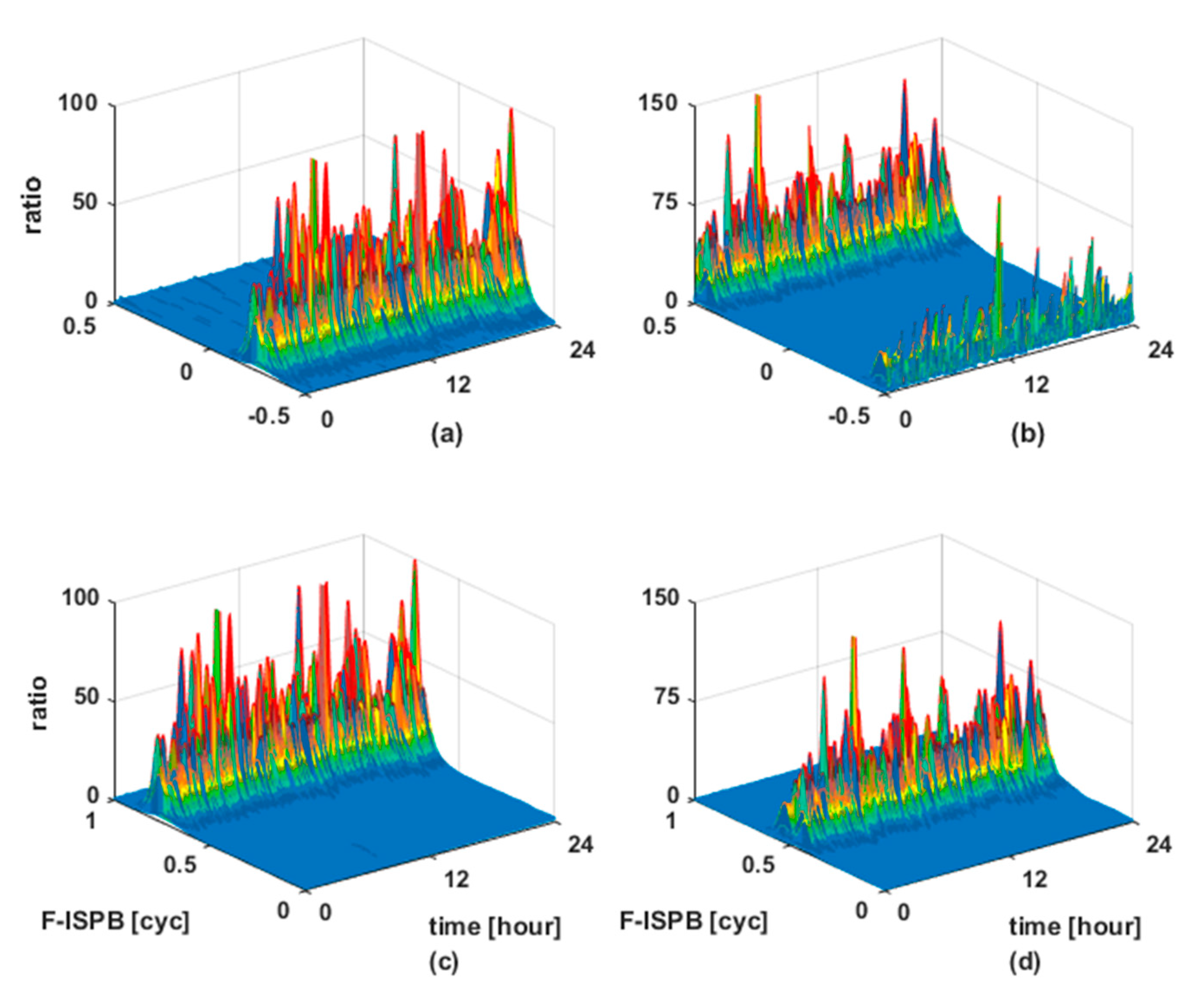
Taking the first epoch from the baseline CUTB–CUTC and CUTB–CUT0 used in subsequent experiments as an example, the relationship between the value of F-ISPB and the value of the ratio is shown in
Figure 1. As can be seen from the figure, the relationship between F-ISPB and ratio presents a unimodal graph. In
Figure 1b, two peaks appear on the boundary of the search space, which will be discussed in a later section. In the figure, the red line is the threshold to determine that the ambiguity has been successfully fixed, and it is generally set to 3.
Figure 2 shows the relationship between the value of F-ISPB and the value of ratio for all epochs of the two baselines. As can be seen from the figure, almost all epochs have roughly the same shape, and the difference only lies in the size of the wave peak. Therefore, the estimation of the F-ISPB problem can be transformed into a single-objective optimal value problem solved by PSO algorithm. Therefore, we can take the value of ratio as the fitness function and use PSO to search the optimal value of F-ISPB.
3.2. Standard Particle Swarm Optimization Algorithm
In the estimation of F-ISPB problem using the standard particle swarm optimization algorithm, the ratio value is used as the fitness function, and each particle is regarded as a solution. The evolution formula of the standard particle swarm optimization algorithm is as follows:
Here, and represent the position and velocity of the ith particle at time t, respectively; is the inertia weight of the particle itself; and are learning factors; and are uniformly distributed random functions within the interval [0,1]; is the historical optimum position of the ith particle itself; is the historical best position of all particles. That is, the velocity renewal of the particle consists of three parts. The first part is the “memory part”: the particle has the inertia of its previous velocity; the second part is the “cognitive part”: the particle’s cognition of its own experience; the third part is the “social part”: particles communicate with each other.
To estimate F-ISPB using PSO algorithm, it is necessary to first determine the population size of particles and its search space range. Too many particles will lead to slow calculation speed, too few particles will easily fall into local optimum. As a rule of thumb, we set the population size to 10.
The integer portion of the phase ISB will be absorbed by the integer carrier phase ambiguity, and the fractional portion may appear anywhere less than one cycle. Therefore, we can fix the particle search space between (−0.5,0.5) cycle.
The simplified steps for F-ISPB estimation using the standard PSO is shown in Algorithm 1. First, calculate the value of
using Formula (6) and initialize 10 particles in the search space. Then, use the value of each particle to correct the value of
, and the LAMBDA method [
36] is used to fix the corrected value. Calculate the ratio value corresponding to each particle, and record the optimal particle. Formula (7) is used to update the state of the particle swarm, and the updated particles will continue to correct the value of
and calculate the value of ratio again. The process of updating the particle swarm state to calculate the value of ratio was repeated ten times. Finally, the particle value corresponding to the optimal ratio value in history is the estimated F-ISPB.
| Algorithm 1 standard PSO to estimate F-ISPB |
1: Calculate by the Formula (6).
2: Initialize 10 particles in search space.
3: Use the value of each particle to correct the value of .
4: Use the LAMBDA method to fix the corrected values.
5: Calculate the value of ratio corresponding to each particle.
6: Record pbest and gbest.
7: For 1:10
Use Formula (7) to update the state of the particles.
Repeat steps 3, 4, 5, and 6.
End for
8: Output: gbest corresponds to F-ISPB. |
3.3. Improved Particle Swarm Optimization Algorithm
When the value of F-ISPB is close to the boundary of search space, the standard particle swarm optimization algorithm is easy to fall into local optimum. To solve this problem, we propose a particle swarm optimization algorithm with adaptive search space.
As shown in
Figure 1a,b, it can be seen from (a) that ratio reaches its maximum value when F-ISPB is around −0.25 cycles. Additionally, it can be seen from (b) that the ratio reaches its maximum value when F-ISPB is around −0.45 cycles. However, since −0.45 is very close to the search area boundary of −0.5, F-ISPB has a local maximum near the other boundary. This will cause PSO to easily fall into local optimum at the boundary and prematurely converge. Additionally, the closer the true value of F-ISPB is to the boundary value, the greater the probability of this phenomenon.
Fortunately, we can transform the search space when the true value of the F-ISPB is close to the search boundary. It is not difficult to derive from Equation (8) that the search space of F-ISPB can be converted from (−0.5,0.5) to (0,1). If the true value of F-ISPB is within the range of (0,0.5), the transformation of the search space will not cause a change in the integer ambiguity. However, if the true value of F-ISPB is (−0.5,0) or (0.5,1), the transformation of the search space will cause a one-cycle change in the integer ambiguity. This will have no effect on the single-epoch location mode. Additionally, it can also be corrected in the multi-epoch location mode.
In
Figure 1, (c) and (d) are the results of (a) and (b) converted from the search space (−0.5,0.5) to (0,1), respectively. It can be seen from (d) that the wave peak originally close to the search boundary is converted to the position close to the search center. The transformation of search space can effectively avoid PSO falling into local optimum.
In addition, according to the stability characteristics of F-ISPB, we propose an improved particle swarm optimization algorithm with elite retention strategy. The value of F-ISPB is stable when the receiver is not restarted [
16,
17]. Therefore, when we initialize all the particles, we can initialize one of the particles to the F-ISPB value that was finally searched by the previous epoch. This will help particles to find the optimal value faster and has a guiding effect on all particles. Even if the receiver is rebooted, it will only make the particle retained by the elite become ordinary particles and will not affect the whole particle swarm search.
The pseudocode simplification process of the improved particle swarm optimization algorithm to estimate F-ISPB is shown in Algorithm 2. First, ten particle individuals are initialized in the search space. If this epoch is not the first epoch, the F-ISPB value estimated from the previous epoch is assigned to one of the particles of this epoch as the elite particle. Then, judge whether the optimal value is located on the boundary of the search space, and if so, transform the search space. The other processes are the same as the standard PSO and will not be described again here.
| Algorithm 2 improved particle swarm optimization to estimate F-ISPB |
1: Calculate by the Formula (6).
2: Initialize 10 particles in search space.
3: If epoch>1
particle 1= elite particle.
End if
4: Use the value of each particle to correct the value of .
5: Use the LAMBDA method to fix the corrected values.
6: Calculate the value of ratio corresponding to each particle.
7: Record pbest and gbest.
8: For 1:10
Use Formula (7) to update the state of the particles.
Repeat steps 4, 5, 6, 7.
End for
9: If gbest in the bounds of the search space.
Transform search space;
Repeat steps 2, 4, 5, 6, 7, 8.
End if
10: Output: gbest corresponds to F-ISPB. |
4. Experiments of Short-Baseline Positioning
In this section, we first test F-ISPB between GPS-L1 and BDS-B1 using improved PSO and standard PSO. Then, the ratio value distribution of the inter-system differenced model based on the improved PSO and the classical intra-system differenced model under different cut-off elevation angles are statistically analyzed. Finally, the ambiguity success rate and positioning accuracy of the three models are compared, respectively. In addition, an inter-system differenced model based on improved PSO is used to test the positioning continuity under receiver restart. In all experiments, the population size of initialized particles is 10, and the maximum number of iteration times is 10, regardless of the improved PSO or the standard PSO. Additionally, the positioning mode all adopts the single-epoch mode. Three sets of short baseline data were selected for the test. The receiver was restarted five times during the IGG01–IGG02 baseline observation. The details of the three short baseline datasets are shown in
Table 1.
It can be seen from
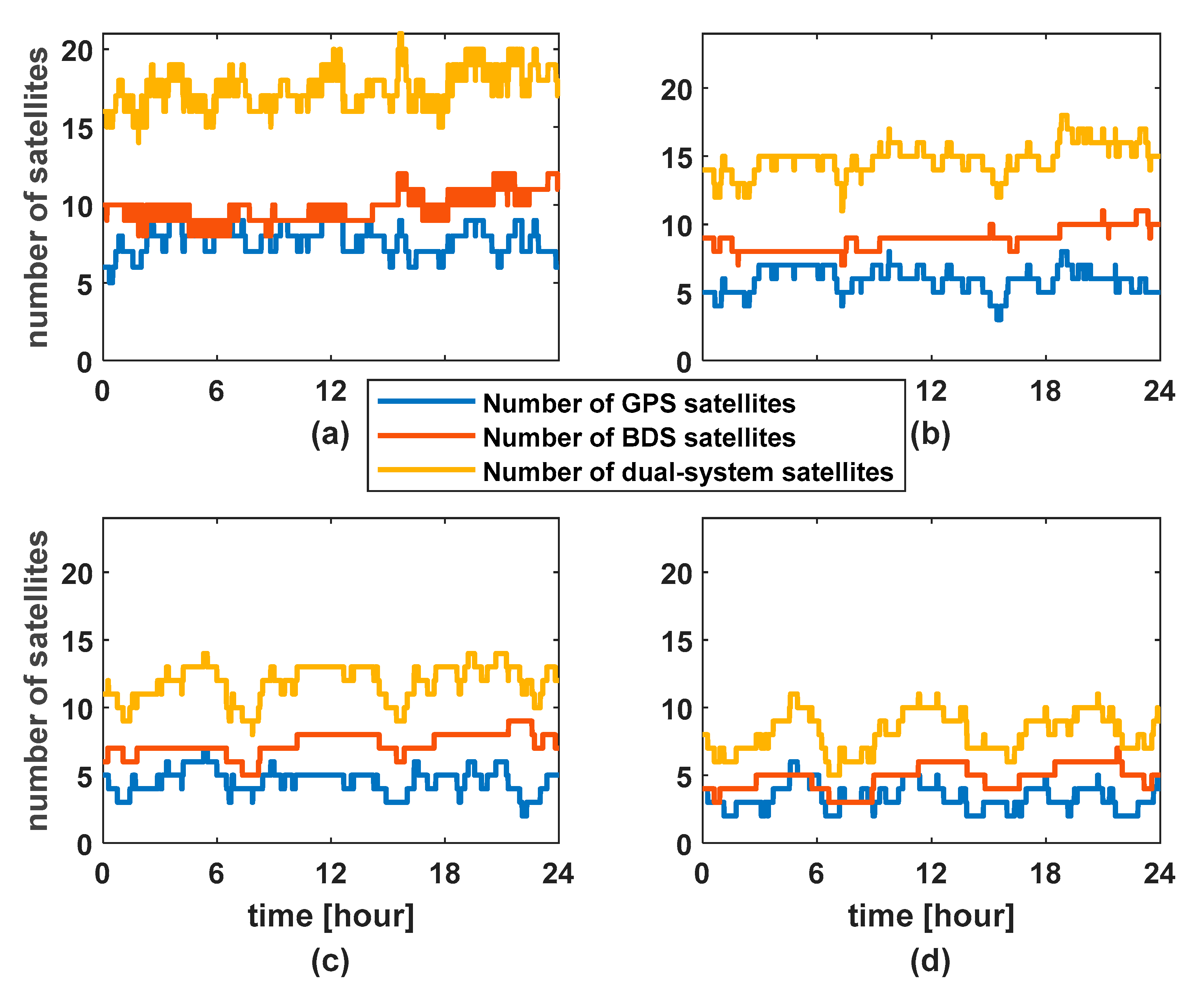
Figure 1 that the CUTB–CUTC baseline is a single peak curve in any search space, while the CUTB–CUT0 baseline may be a multi-peak curve. Therefore, we choose CUTB–CUT0 baseline to do experiments to verify the superiority of the improved PSO. The number of BDS and GPS visible satellites at the CUTB–CUT0 baseline is shown in
Figure 3.
Figure 3a–d, respectively, represent the number of satellites when the cut-off elevation angle is 15, 25, 35, and 45 degrees. As can be seen from the figure, the number of visible satellites decreases sharply with the increase in the cut-off elevation angle of satellites. Most epochs have more than 15 satellites when the cut-off elevation angle is 15 degrees; most epochs have about 15 satellites when the cut-off elevation angle is 25 degrees; most epochs have about 12 satellites when the cut-off elevation angle is 35 degrees; when the cut-off elevation angle is 45 degrees, the number of satellites decreases sharply, and a single epoch only has five, so the single system cannot be solved.
The F-ISPB results of CUTB–CUT0 baseline estimation using PSO are shown in
Figure 4.
Figure 4a shows the F-ISPB estimated results in the search space (−0.5,0.5) cycles using the standard PSO. Since the actual F-ISPB is about 0.47 cycles, it is easy to fall into local optimum around −0.5 cycles when using the standard PSO algorithm. Therefore, a large number of epochs appear in the figure, and the F-ISPB value estimated by the epochs is around −0.5 cycles.
Figure 4b shows the F-ISPB estimation results of the PSO for the adaptive search space. As can be seen from the figure, the PSO algorithm of the adaptive search space converts the search space into (0,1) cycles. The estimated results of most epochs are around 0.47 cycles, but there are still a few deviations, which may be due to too few cycles to find the optimal solution.
Figure 4c shows the F-ISPB estimation results of the PSO for the elite retention strategy in the search space (−0.5,0.5) cycles. As can be seen from the figure, compared with the standard PSO, the estimated value of F-ISPB by the PSO for the elite reservation strategy is better in the situation that the value of F-ISPB falls into local optimum. However, there are still many epochs that fall into local optimality.
Figure 4d is the F-ISPB estimation result using the improved PSO algorithm proposed in this paper. This method has both elite retention strategy and adaptive search space function. As can be seen from the figure, the estimated results of almost all epochs are clustered around 0.47 cycles, and the results of
Figure 4d are more clustered than that of
Figure 4b without the elite retention strategy.
All epochal ratio values of CUTB–CUT0 baseline obtained by using the inter-system differenced model based on improved PSO and classic intra-system differenced model at different cut-off elevation angles are shown in
Figure 5.
Figure 5a–d, respectively, represent the ratio value obtained by using the two methods when the cut-off elevation angle is 15, 25, 35, and 45 degrees. As can be seen from the figure, when the cut-off elevation angle is 15 degrees and 25 degrees, the difference in the ratio value between the two models is not obvious. This is because there are a large number of visible satellites at this time, so the advantage of inter-system differenced model over intra-system difference model is not obvious. When the cut-off elevation angle is 35 degrees and 45 degrees, the ratio value of the inter-system differenced model based on the improved PSO is improved as a whole compared with the classical intra-system differenced model. Especially when the cut-off elevation angle is 45 degrees, the improvement is more obvious. This is because the number of visible satellites is rare at this time, so the inter-system differenced model has better model strength compared with the intra-system differenced model. Especially when the cut-off elevation angle is 45 degrees, the number of visible satellites of all epochs is 10 or less.
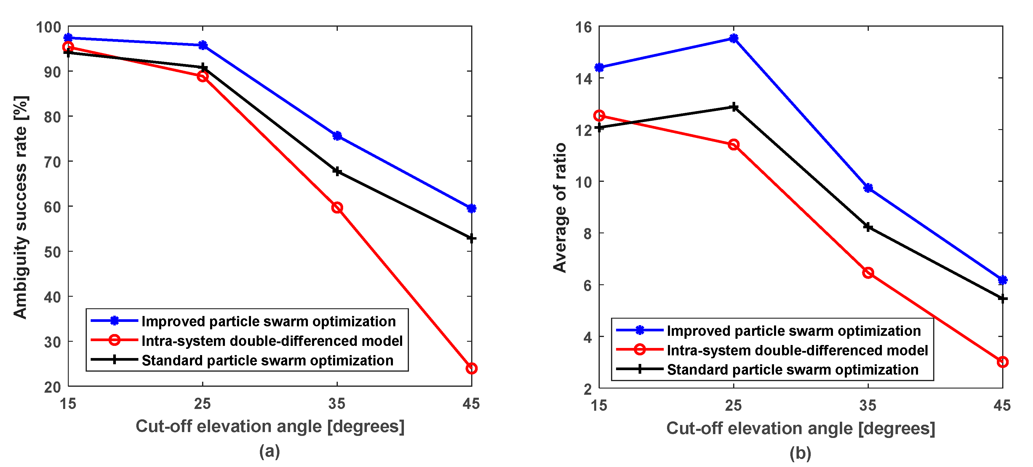
Figure 6 shows the ambiguity success rate and average of ratio obtained by using three models to process the CUTB–CUT0 baseline at different cut-off elevation angles. As can be seen from
Figure 6a, when the cut-off elevation angle is 15 degrees and 25 degrees, the ambiguity success rate of the inter-system differenced model based on the improved PSO is slightly higher than that of the other two methods. When the cut-off elevation angle is 35 and 45 degrees, the ambiguity success rate of the inter-system differenced model based on the improved PSO is much higher than the other two methods, especially the classical intra-system difference model. As can be seen from
Figure 6b, at any cut-off elevation angle, the average ratio of the inter-system differenced model based on the improved PSO is higher than that of the other two methods. When the cut-off elevation angle is 15 degrees, the average ratio of the classical intra-system differenced model is slightly higher than the inter-system difference model based on the standard PSO. However, at other cut-off elevation angles, the ratio value of the inter-system differenced model based on the standard PSO is higher. It is not difficult to find that the less the number of satellites, the advantages of the inter-system differenced model will be more obvious than that of the intra-system differenced model. Additionally, compared with the standard PSO, the improved PSO has further improved the ambiguity success rate and the average ratio.
Three methods were used to process the CUTB–CUT0 baseline, and the processing mode is all single-epoch mode.
Table 2 shows the percentage of epochs with positioning errors less than 1cm and 5cm at different cut-off elevation angles. It can be seen from the table that the inter-system differenced model based on the improved PSO is better than the other two methods no matter what the cut-off elevation angle. With the increase in the cut-off elevation angle and the decrease in the number of visible satellites, the lifting effect becomes more obvious. However, it can be seen from the table that the positioning effect of the inter-system differenced model based on the standard PSO is not as good as that of the classical intra-system differenced model at any cut-off elevation angle. This is because the standard PSO always falls into local optimum when searching for F-ISPB, and the value of F-ISPB has a great influence on the positioning effect. In terms of positioning accuracy, the same conclusion as the above experiments can be obtained, that is, the less the number of visible satellites is, the more obvious the advantage of the inter-system difference model based on the improved PSO is.
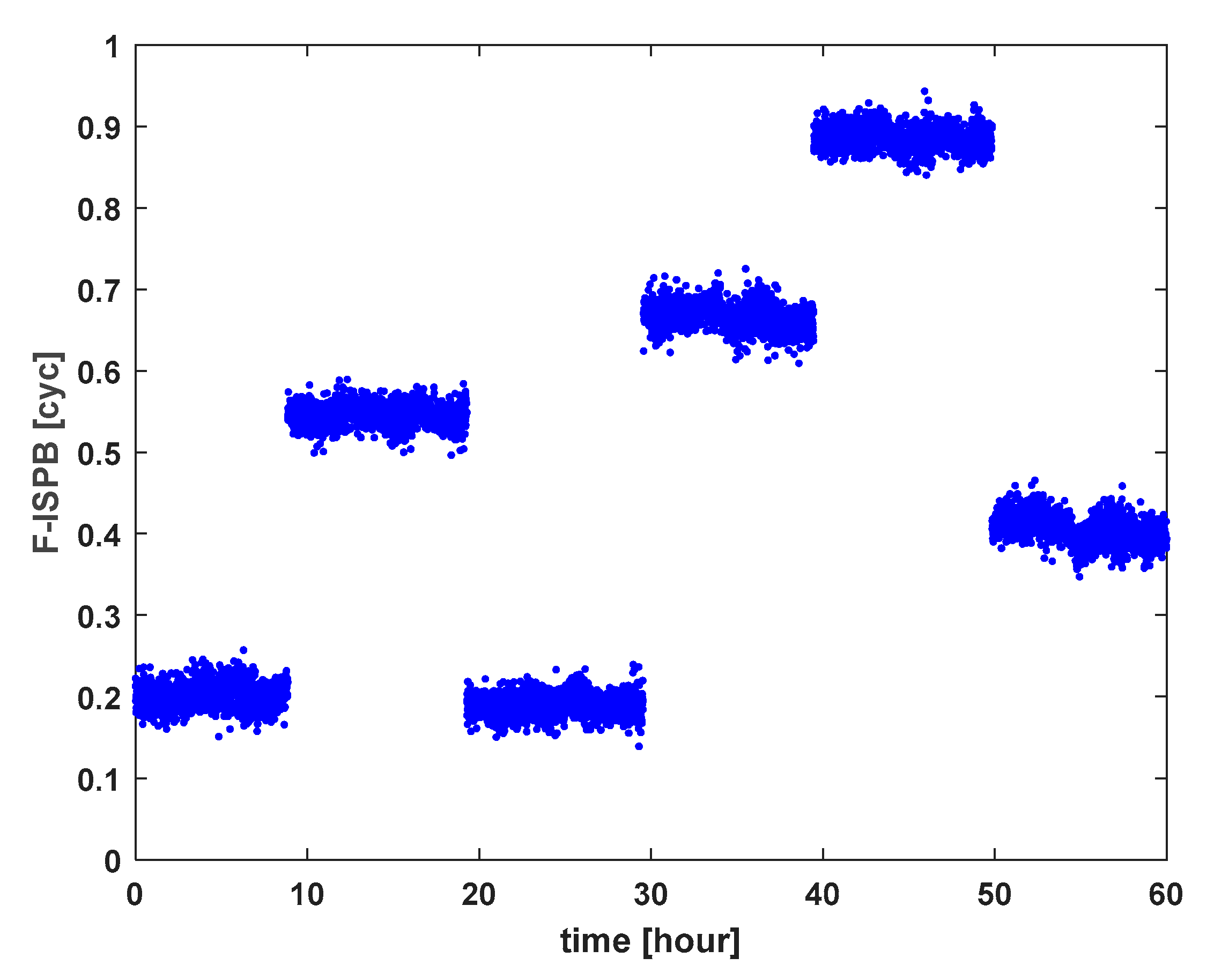
The F-ISPB results of IGG01–IGG02 baseline estimation using improved PSO are shown in
Figure 7. The IGG01–IGG02 baseline underwent a total of five receiver restarts during the observation period. Therefore, we can see from the figure that the value of F-ISPB jumps five times in total. Additionally, after each restart, the improved PSO can still estimate the value of F-ISPB quickly and accurately. Therefore, the inter-system differenced model based on the improved PSO can be used to estimate F-ISPB accurately in real time and ensure the continuity of positioning without being affected by receiver restart. For the data from the fourth restart to the fifth restart, the search space is in (−0.5,0.5) weeks, and its F-ISPB is around −0.1 cycles. For the sake of intuition, Formula (8) has been used in the figure to convert it into the search space of (0,1) cycles.
5. Conclusions
In this paper, we propose an improved particle swarm optimization (PSO) algorithm with adaptive search space function and elite reservation strategy to estimate F-ISPB. This method can accurately estimate the F-ISPB in real time in the single-epoch positioning mode, even in the case of receiver restart. This will greatly increase the robustness of the inter-system differenced model applied in real complex scenarios.
Compared with the standard PSO, the improved PSO proposed in this paper can effectively avoid particles falling into local optimum prematurely. The adaptive search space function can transform the particle swarm into another search space for exploration when the F-ISPB value is close to the search boundary. After transforming the search space, the F-ISPB value will not be close to the boundary of the search space, which can effectively avoid the particle swarm falling into local optimum. Since the integer part of the ISPB will be absorbed by the integer carrier phase ambiguity, the effect of positioning will not be affected by the transformation of the search space. Because the F-ISPB value has good stability, it makes it possible to put forward the elite retention strategy. The elite retention strategy can make the particle swarm converge faster and more accurately. Even if the receiver is restarted, the elite particles will not affect the re-estimation of the F-ISPB value.
Compared with the classical intra-system differenced model, the inter-system differenced model based on improved PSO increases the redundant observations and improves the strength of the model. The inter-system differenced model based on improved PSO is superior to the classical intra-system differenced model in both ambiguity success rate and positioning accuracy. Additionally, the fewer the number of visible satellites, the more obvious the advantage of the difference model between systems.


