Abstract
Total sea level changes from space radar altimetry are mainly decomposed into two contributions of mass addition and volume expansion of oceans, measured by GRACE space gravimeter and Argo float array, respectively. However, the averages of altimetry, mass, and steric sea level changes have been usually examined over the respective data domains, which are different to one another. Errors arise from this area inconsistency is rarely discussed in the previous studies. Here in this study, an alternative definition of ocean domain is applied for examining sea level budgets, and the results are compared with estimates from different ocean areas. It shows that the impact of area inconsistency is estimated by about 0.3 mm/yr of global trend difference, and averages based on a consistent ocean area yield a closer agreement between altimetry and mass + steric in trend. This contribution would explain some discordances of past sea level budget studies.
1. Introduction
Sea level change is an important indicator of global climate change, and the rate is currently increasing due to ongoing global warming. Ocean mass increase and volume expansion are well-known as significant contributors to the global mean sea level (GMSL) rate [1]. Recent studies have shown that ocean mass addition is the more significant cause of present-day GMSL rise, accounting for two-thirds of the rate for 2002–2017 [2]. Total sea level change has been monitored by satellite radar altimetry since 1993. Density-driven volumetric sea surface height change (i.e., steric change) is estimated from ocean temperature and salinity changes, and the profiles have been measured by in situ Argo float array since 2000 [3]. Ocean mass changes have been measured by space gravimeters of Gravity Recovery and Climate Experiment (GRACE) and GRACE Follow-On missions since 2002 [4,5]. In particular, the distribution of ocean mass change is closely associated with geoid change, resulting from both solid and hydrological mass redistribution of the Earth. A number of recent studies have compared these three complementary data sets and showed that altimetry measurements generally agree well with the sum of mass changes from GRACE and steric changes from Argo data in terms of the global averages [6,7,8,9].
However, it is notable that these data sets do not fully cover global oceans, and further, the data coverages are considerably different from one another. For example, altimetry data processing uses a number of measurements from different satellites, and the averaged data is usually provided over a reduced latitude range of ±66°, because of orbital inclination of satellites, such as TOPEX/Poseidon and Jason-1 to -3, whose measurements are importantly used in the processing [10]. Although other satellites with the larger inclination (such as ERS-1 and -2, Cryosat, Envisat, etc.) cover near-polar regions (up to ~80°), the measurements show a limited performance, particularly associated with the presence of sea ice in high-latitude oceans [11,12]. Ice-covered oceans also limit Argo float deployments; the spatial coverage and density of the array become relatively complete after 2005, but still, the Arctic Sea remains uncovered [2]. Further, most Argo data sets provide ocean temperature and salinity profiles usually from 0 to 2000 m depth, and measurements in shallow water are sometimes missing. On the other hand, GRACE data nominally covers global oceans, but the effective resolution of the data is relatively low due to the post-processing steps, which were introduced to suppress errors in spatially high frequency signals [13,14]. These methods lower the resolution and cause significant signal leakages mostly from land to oceans, contaminating ocean mass changes up to hundreds of kilometers away from coastlines. Thus, many GRACE sea level studies have employed a reduced global ocean without the coastal band to exclude the leakage contribution [15].
Despite the different coverage of data sets as explained above, many studies routinely use the averages of altimetry, Argo, and GRACE examined over the respective data domains when investigating global sea level budget (e.g., [9,16,17]). Such schemes may assume that sea level changes at the marginal areas are not quite different from the changes over the observation area, or may be an attempt to obtain an estimate based on maximum data availability. However, GRACE data coverage is generally more extensive than altimetry and Argo ocean domains, and the inconsistency would result in additional misfits in the linearly combined sea level budget. Averages over an area consistently applicable for all data sets would reduce the errors and provide more reasonable decomposition of sea level rate into mass- and density-driven contributions over a fixed near-global area. In this study, sea level changes from three data sets of altimetry, Argo steric, and GRACE data are examined considering consistent area definition of the global ocean domain. The results are compared with conventional estimates (based on different data domains) and examine which ocean definition leads to the closer agreement of the sea level budget.
2. Materials and Methods
2.1. Data
In this study, multiple data sets of altimetry, Argo, and GRACE were considered to obtain reasonable estimates of total, steric, and mass sea level changes, respectively. For example, a mean value of several altimetry data sets represents the total sea level change estimate. Such averaging is also called an ensemble mean, which effectively suppress random noises and errors associated with different data processing methods of data centers [17].
Altimetry data sets provided from four different institutes were considered in this study: Copernicus Marine Environment Monitoring Service (CMEMS) [18]; Climate Change Initiative (CCI) [19]; Commonwealth Scientific and Industrial Research Organization (CSIRO) [20]; and Jet Propulsion Laboratory (JPL) [21]. Since the glacial isostatic adjustment (GIA) effect is included in these altimetry observations, the contribution was manually corrected by using a gridded trend map of ICE6G-D model [22]. Hereafter, ΔA denotes total sea level change obtained from averaging these GIA-corrected altimetry data sets.
In a similar manner, three Argo temperature and salinity profiles (0 to 2000 m depth) were averaged to obtain steric sea level change ΔS. They were provided from International Pacific Research Center (IPRC), Japan Agency for Marine-Earth Science and Technology (JAMSTEC) [23], and Scripps Institution of Oceanography (SIO) [24].
Mass sea level change estimates (denoted by ΔM) have been widely investigated from GRACE level-2 GSM products. As mentioned above, GSM data includes a significant leakage effect in the reduced data after post-processing. Thus, GRACE Mascon data was used here for ΔM estimates. Mascon solutions are improved mass change distributions that consider signal leakage correction in the data processing to provide high-resolution mass changes, and ocean mass signals are globally available without discarding the coastal band. Here, three different GRACE Mascons were averaged to yield ΔM estimates: RL06 Mascons from Center for Space Research (CSR) [25], RL06 v02 Mascons from Jet Propulsion Laboratory (JPL) [26], and v02.4 Mascons from Goddard Space Flight Center (GSFC) [27]. GIA correction of CSR and JPL Mascons considers the same model (ICE6G-D) as applied for altimetry. Although the GSFC Mascons used in the present analysis use ICE6G-C [28], it is almost identical to ICE6G-D model over oceans. The ocean signals are restored by using GAD contribution, which indicates the effect of mass redistribution due to ocean dynamics and atmospheric pressure changes from Atmosphere and Ocean De-aliasing (AOD) 1B background model [29]. The monthly ocean mean of GAD is subtracted for Inverse-Barometer (IB) correction [30].
Three data sets of ΔA, ΔS, and ΔM were equally converted to monthly solutions from January 2005 to December 2015, on 1 × 1° grids. Sea level budget was simply evaluated by an equation that ΔA = ΔS + ΔM + errors. Since this study focuses on the trend agreement, seasonal variabilities were removed from all data sets. Other effects, such as ocean floor deformation due to global surface mass load [31] and steric changes due to deep oceans (below 2000 m depth) [32] were not included considering the small contributions to the global rates. Errors from these factors are discussed in Section 4.
2.2. Area-Weighted Average for Global Sea Level Changes
Mean sea level changes over a specific area are normally examined by using the area-weighted average. Let a mean value of sea level data averaged over an ocean area at time , and it is described by
where represents any data set of altimetry, Argo steric, and GRACE data, and indicates a unit area of the spherical earth, such as for colatitude , longitude , and the Earth’s radius . Here, is an ocean function; it is one at the oceans, and is zero otherwise. We can obtain global mean when covers the entire ocean.
As shown in Equation (1), a global mean in principle requires both data integration and averaging over global ocean . However, as explained above, ΔA, and ΔS data sets are not fully provided over domain, due to the limited measurements. Many studies for sea level budgets practically examine “global mean” using the maximum data availability of individual data sets. The formulations are
for altimetry sea level changes,
for steric changes, and
for ocean mass changes, where , , and represent the data domains of altimetry, Argo steric, and GRACE data, respectively. As shown in Equations (2)–(4), the averages are obtained over different areas. The estimates have been routinely compared in many sea level budget studies, supposing that . The difference among the areas is likely to create additional errors when examining sea level budget.
In order to reconcile the area inconsistency, here an alternative ocean domain is defined; it indicates common data coverage of all data sets. It allows evaluating mean changes of all data sets over a consistent area:
Sea level budgets using Equation (5) would substantially reduce errors associated with the inconsistency of ocean domains. In the Results Section below, sea level budgets from conventional averaging methods (using Equations (2)–(4)) will be compared with the result from Equation (5).
3. Results
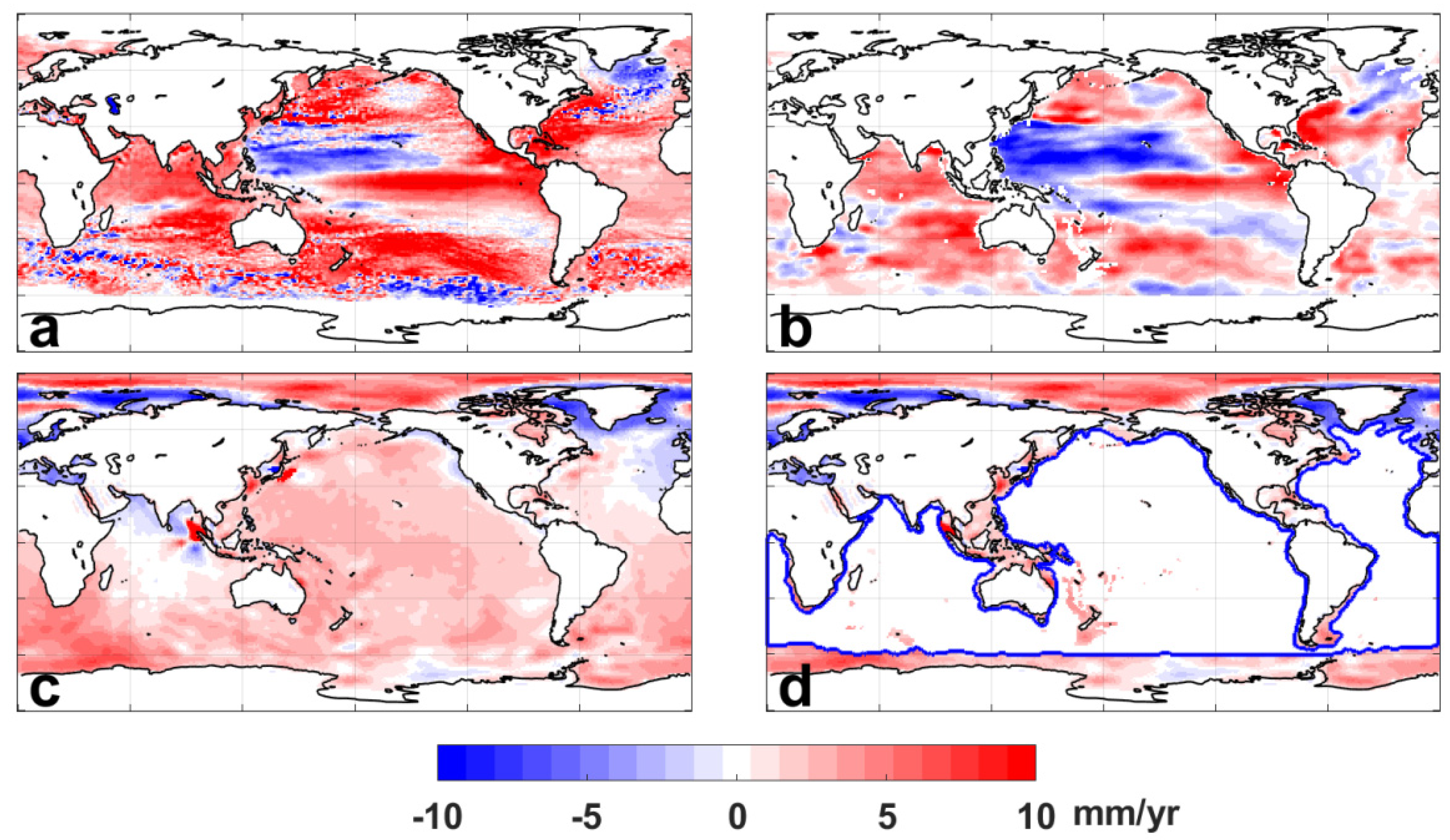
Figure 1 is trend maps of altimetry, Argo steric, and GRACE Mascon solutions, showing typical data coverage of each data set. Figure 1a is the sea level trend estimated from CMEMS altimetry data; the coverage is similar but not equal to other altimetry domains provided from JPL, CCI, and CSIRO. These altimetry data sets cover ~90% of the global ocean area, commonly excluding the Arctic Ocean and the Antarctic Ocean. Figure 1b shows the steric sea level trend estimated by the JAMSTEC product. As seen in the Figure, the data does not provide estimates over oceans in the polar region, the Mediterranean Sea, continental shelf near the East and Southeast Asia and Zealandia, etc. There are also differences in the definitions of IPRC and SIO ocean domains. For example, IPRC and SIO data do not cover the Caribbean Sea. The data coverages of these Argo steric data range from 76% to 83% of the global ocean. Figure 1c shows the ocean mass trend of CSR Mascon data, and the data is available over almost the entire ocean area as JPL and GSFC Mascons. Figure 1a–c shows that the data domains of three complementary data sets are significantly different from one another, particularly in high-latitude oceans. Thus, using averages over these different ocean domains for the linear sea level budget equation of ΔA = ΔS + ΔM would involve errors from the domain inconsistency. Other regions may have a minor impact, but the contribution of the high-latitude oceans would result in significantly different estimates. For example, the trend of CSR Mascons outside a common data coverage D′ is shown in Figure 1d. Area D′, whose outer boundary is indicated by the thick blue line, is defined by common data availability of all data sets used in the present analysis (four altimetry data, three Argo steric changes, and three GRACE Mascons). As shown in Figure 1d, ocean mass changes from CSR Mascons outside the altimetry and Argo coverages included a significantly lower trend mostly in the Arctic Ocean. Over this marginal area, the regional mass rate of CSR Mascons were about 1.20 mm/yr, while the estimate over area D′ was about 1.88 mm/yr. JPL and GSFC Mascons were estimated by about 0.88 and 1.72 mm/yr of mass rate in the marginal area. These were also lower than the estimates over area D′ (2.20 and 2.01 mm/yr, respectively). Due to these small rise rates over the high-latitude oceans, mass rate over the global ocean (by the definition of Mascons) become smaller than the estimate over altimetry and Argo domain (area D′).

Figure 1.
Trend maps of (a) altimetry data provided from CMEMS, (b) Argo steric data from JAMSTEC, and (c) GRACE CSR Mascons (GAD included after considering IB correction). (d) Trend map of CSR Mascons outside ocean domain , whose outer boundary is indicated by a thick blue line. Area is commonly available for all data sets considered in this study (altimetry data from CMEMS, CCI, CSIRO, and JPL; Argo steric data from IPRC, JAMSTEC, and SIO; and GRACE Mascon solutions from CSR, JPL, and GSFC). The trends are estimated by using linear regression after removing seasonal variations.
First, sea level estimates were evaluated using conventional global averaging method (with respect to different data coverages, ignoring domain inconsistency). The results are displayed in Figure 2. The time series of ΔA (gray solid curve), ΔS (red), and ΔM (blue) are ensemble mean values of four altimetry data, three Argo steric data, and three Mascon solutions, respectively. Individual estimates of each data set are given in the third column of Table 1. The sum of ΔS and ΔM indicated by the black solid curve is compared with the ΔA estimate. As shown in the Figure, there is a significant trend disagreement between ΔA and ΔS + ΔM estimates by ~0.5 mm/yr. The misfit is even larger than the sea level rise contribution due to the total ice mass loss of Antarctica (~0.4 mm/yr) estimated in a previous study [33]. Explaining the difference based on this result would lead to the overestimation of missing contributions (e.g., deep steric effect, load deformation of the ocean floor, etc.).
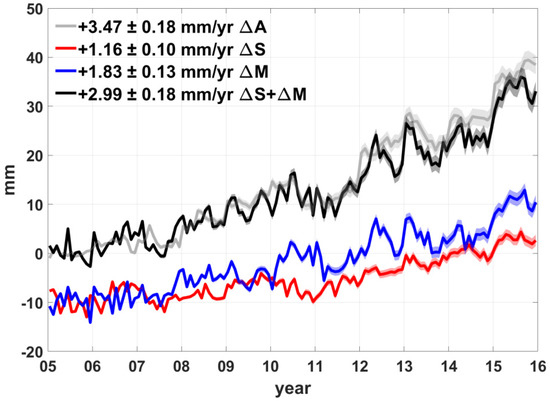
Figure 2.
Ensemble mean of sea level change estimates of altimetry (ΔA, gray curves), Argo steric (ΔS, red), and GRACE Mascons (ΔM, blue). The sum of ΔS and ΔM contributions are presented with a black solid curve. The computations are based on Equations (2)–(4) with respect to individual data domains as provided, and the detailed evaluation is listed in Table 1. The trends are estimated by using linear regression after removing seasonal variations. Error boundaries are given at 95% confidence level, shown as shaded plots along with the corresponding curves. Red and blue curves include negative offsets (−10 mm) for clarity.

Table 1.
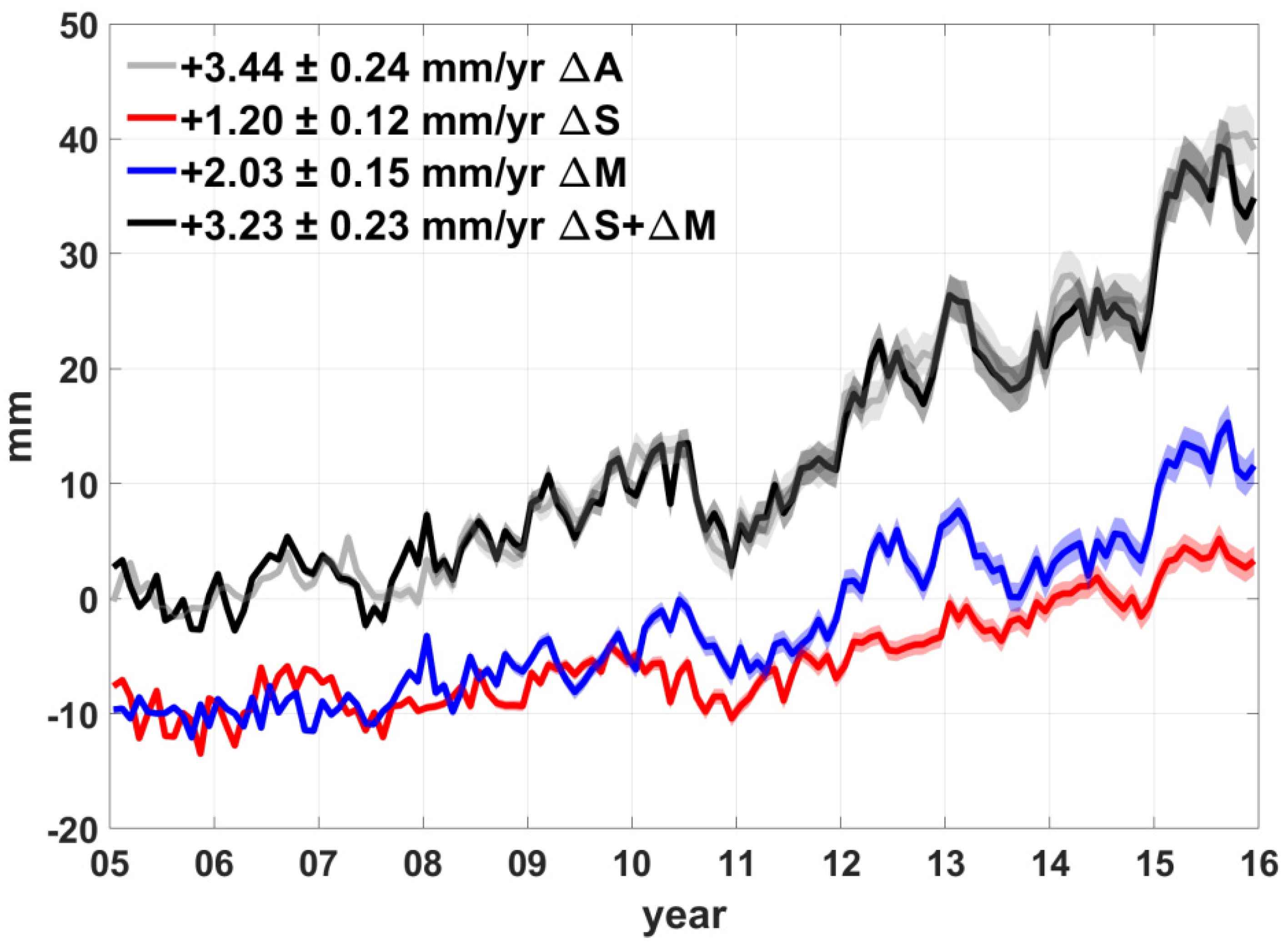
Trend estimates of all data sets used in this study with respect to ocean domains. Maximum data coverages of individual data sets are used to yield estimates in the third column, and the ensemble mean values (bolded numbers) are used for Figure 2.Results in the fourth column are consistently estimated over the common data coverage defined in this study, with the plots shown in Figure 3. Estimates of ΔA and ΔM consider GIA correction using the same model of ICE6G-D. The trends are estimated by using linear regression after removing seasonal variations. Error boundaries are given at 95% confidence level.
Now we evaluate a sea level budget using a consistent area and the result is shown in Figure 3. Estimates from individual data sets are listed in the fourth column of Table 1. The trend estimates are different compared to Figure 2. The reconstructed sea level budget of ΔS + ΔM presented in Figure 3 is much closer to the measurement of ΔA, differing only by ~0.2 mm/yr. The improvement is mostly due to ΔM contribution. Since area is quite close to and , estimates of ΔA and ΔS trends are almost equal to the previous results shown in Figure 2. On the other hand, ΔM estimate increases by ~0.20 mm/yr in Figure 3, and it mainly contributes to the better agreement with ΔA. The difference is due to the excluded contribution of the polar region from area definition, previously shown in Figure 1d. Many studies have demonstrated that mass sea level changes in the polar region would decrease due to descending geoid height [31,34,35,36]. There, local gravity is rapidly declining due to ongoing ice mass loss in Greenland and Antarctica, and ocean mass is redistributed along the declining geoid surface. Thus, the average ocean mass rate without the high-latitude oceans generally gives a larger trend estimate, and the difference accounts for ~0.20 mm/yr according to the average of three Mascon solutions. Altimetry measurements ought to capture this effect, but it is outside an ordinary altimetry coverage (). Thus, sea level budgets considering different ocean domains of , , and therein involve errors from missing contribution of this distinct gravity-induced effect, only captured in ΔM contribution. Contrarily, estimates of ΔA and ΔS + ΔM based on area yield a closer agreement due to equal treatment for high-latitude oceans in the area definition. The estimates are provided over reduced near-global oceans (covering ~75% of the global ocean) but are free of uncertainties associated with domain inconsistency.

Figure 3.
Similar to Figure 2, but from averaging over consistent data coverage as defined in Equation (5).
4. Discussion
Averages over a consistent area provide a closer agreement between altimetry and Argo + GRACE within error boundaries (95% confidence level). This result indicates that inconsistency of ocean domain has contributed to some trend misfits in the previous sea level budget studies. Further, the errors due to area inconsistency may be mistaken for contributions from other causes.
The estimates shown in the Figure can be changed depending on the choice of data sets. Ensemble mean values from more various altimetry, Argo, and GRACE data sets further reduce errors from different processing methods and models used for each data set. Considering missing contributions also yields different trend estimates. For example, it is expected that the reconstructed rate is slightly decreased by -0.13 ± 0.01 mm/yr or more when considering global load deformation of ocean floor [31]. Deep steric change (below 2000 m depth) omitted from the present analysis would add +0.12 ± 0.03 mm/yr [37] or more [32] to the estimate. Mascon solutions include non-surficial processes like earthquake signals, as seen in Figure 1, and the treatment would yield a minor impact on the global sea level trend. Tang et al. [38] examined that the correction accounts for −0.07 ± 0.02 mm/yr of global rate. Other unmodeled tidal effects in GRACE data could contribute to the misfit [39].
Note that the estimate shown in Figure 3 is not for “global” estimates, because the high-latitude ocean is missing from the ocean definition of . The total sea level rate in the polar region is possibly lower than the global estimate. First, local gravity decrease due to massive ice mass loss in Greenland and Antarctica results in the lower (or negative) average mass rate in the polar region. As shown in Section 3, the contribution based on Mascon solutions creates ~0.2 mm/yr of global rate difference between cases with and without the regions. Secondly, freshwater addition due to ice melt can result in additional steric changes in high-latitude oceans. For example, salinity decrease due to meltwater inflow (i.e., freshening) causes volume expansion [40,41]. Previous studies found that this halosteric component (steric changes due to salinity variation) dominantly affects the spatial pattern of steric sea level trend in the Arctic Ocean (from 66° N to 80° N), but the regional average is lower than the global mean steric rate because the positive and negative trend patterns offset each other [11]. Considering these steric and mass contributions in the polar region, the true global sea level trend over the entire ocean would become smaller than the rise rates presented in Figure 3.
5. Conclusions
Using multiple altimetry, Argo steric, and GRACE Mascon solutions, this study examines sea level budgets using two different definitions for the ocean domain. Following a conventional method attempted in the previous studies, one evaluates mean values over oceans individually defined in altimetry, Argo, and GRACE data sets, recognizing that the domains are considerably different from each other. Another examination employs a consistent ocean area where all three data sets are available. The comparison shows that altimetry measurements agree more with Argo steric plus GRACE Mascons in trend when a consistent ocean area is applied. The ocean domain adjustment adds ~0.2 mm/yr of trend in the reconstructed sea level change (Argo + GRACE). The improvement is mainly due to consistent treatment for ocean area in the polar region, which includes gravitational ocean mass decrease. Contrary to GRACE observation, average sea level change from altimetry does not include the contribution due to the limited spatial coverage of measurement. This result implies that past sea level budgets considering different ocean definitions possibly involve errors associated with the inconsistency of applied ocean domains. Since spatial coverages of altimetry, Argo steric, and GRACE data are significantly different from one another, sea level budget examined over a common data coverage effectively reduces the uncertainties and allows accurate decomposition of sea level rise contributions.
Funding
This research was funded by the Korea Institute of Marine Science and Technology promotion (KIMST) research grant (PM20020) and the National Research Foundation of Korea (NRF) grant (No. 2020R1A2C2006857).
Data Availability Statement
Mascon solutions from CSR, JPL, and GSFC can be obtained from GRACE Tellus website, https://grace.jpl.nasa.gov/data/get-data (accessed on 12 August 2021). CMEMS altimetry data is distributed from http://marine.copernicus.eu/services-portfolio/access-to-products (accessed on 12 August 2021). CCI altimetry data is provided from https://catalogue.ceda.ac.uk/uuid/142052b9dc754f6da47a631e35ec4609 (accessed on 12 August 2021). CSIRO altimetry data can be downloaded at http://www.cmar.csiro.au/sealevel/sl_data_cmar.html (accessed on 12 August 2021). JPL altimetry data, Gridded Sea Surface Height Anomalies Climate Data Record Version JPL 1609, is distributed from http://podaac-tools.jpl.nasa.gov/drive/files/allData/merged_alt/L4 (accessed on 12 August 2021). Argo data sets from IPRC, JAMSTEC, and SIO are all accessible via http://argo.ucsd.edu/data/argo-data-products (accessed on 12 August 2021). ICE6G GIA models are available at Peltier’s website, http://www.atmosp.physics.utoronto.ca/~peltier/data.php (accessed on 12 August 2021).
Acknowledgments
I deeply appreciate Academic Editor, Fracesco Serafino, and three anonymous reviewers who helped to improve this manuscript. Further, special thanks to Ki-Weon Seo, who provided constructive comments.
Conflicts of Interest
The author declares no conflict of interest.
References
- Church, J.A.; Clark, P.U.; Cazenave, A.; Gregory, J.M.; Jevrejeva, S.; Levermann, A.; Merrifield, M.A.; Milne, G.A.; Nerem, R.S.; Nunn, P.D.; et al. Sea Level Change. In Climate Change 2013: The Physical Science Basis; Contribution of Working Group I to the Fifth Assessment Report of the Intergovernmental Panel on Climate Change; Stocker, T.F., Qin, D., Plattner, G.-K., Tignor, M., Allen, S.K., Boschung, J., Nauels, A., Xia, Y., Bex, V., Midgley, P.M., Eds.; Cambridge University Press: Cambridge, UK; New York, NY, USA, 2013; pp. 1137–1216. [Google Scholar]
- Chen, J.; Tapley, B.; Save, H.; Tamisiea, M.E.; Bettadpur, S.; Ries, J. Quantification of Ocean Mass Change Using Gravity Recovery and Climate Experiment, Satellite Altimeter, and Argo Floats Observations. J. Geophys. Res. Solid Earth 2018, 123, 212. [Google Scholar] [CrossRef]
- Roemmich, D.; Owens, W.B. The Argo Project: Global Ocean Observations for Understanding and Prediction of Climate Variability. Oceanography 2000, 13, 45–50. [Google Scholar] [CrossRef] [Green Version]
- Tapley, B.D.; Bettadpur, S.; Watkins, M.; Reigber, C. The gravity recovery and climate experiment: Mission overview and early results. Geophys. Res. Lett. 2004, 31, L09607. [Google Scholar] [CrossRef] [Green Version]
- Landerer, F.W.; Flechtner, F.M.; Save, H.; Webb, F.H.; Bandikova, T.; Bertiger, W.I.; Bettadpur, S.V.; Byun, S.H.; Dahle, C.; Dobslaw, H.; et al. Extending the Global Mass Change Data Record: GRACE Follow-On Instrument and Science Data Performance. Geophys. Res. Lett. 2020, 47, 088306. [Google Scholar] [CrossRef]
- Cazenave, A.; Dieng, H.-B.; Meyssignac, B.; Von Schuckmann, K.; Decharme, B.; Berthier, E. The rate of sea-level rise. Nat. Clim. Chang. 2014, 4, 358–361. [Google Scholar] [CrossRef]
- Chen, J.L.; Wilson, C.R.; Tapley, B. Contribution of ice sheet and mountain glacier melt to recent sea level rise. Nat. Geosci. 2013, 6, 549–552. [Google Scholar] [CrossRef]
- Dieng, H.B.; Cazenave, A.; Von Schuckmann, K.; Ablain, M.; Meyssignac, B. Sea level budget over 2005–2013: Missing contributions and data errors. Ocean Sci. 2015, 11, 789–802. [Google Scholar] [CrossRef] [Green Version]
- WCRP. Global Sea-Level Budget 1993–Present. Earth Syst. Sci. Data 2018, 10, 1551–1590. [Google Scholar] [CrossRef] [Green Version]
- Benveniste, J.; Birol, F.; Calafat, F.; Cazenave, A.; Dieng, H.; Gouzenes, Y.; Legeais, J.F.; Léger, F.; Niño, F.; Passaro, M.; et al. Coastal Sea Level Anomalies and Associated Trends from Jason Satellite Altimetry over 2002–2018. Sci. Data 2020, 7, 357. [Google Scholar]
- Carret, A.; Johannessen, J.A.; Andersen, O.B.; Ablain, M.; Prandi, P.; Blazquez, A.; Cazenave, A. Arctic Sea Level During the Satellite Altimetry Era. Surv. Geophys. 2017, 38, 251–275. [Google Scholar] [CrossRef]
- Cheng, Y.; Andersen, O.; Knudsen, P. An Improved 20-Year Arctic Ocean Altimetric Sea Level Data Record. Mar. Geod. 2014, 38, 146–162. [Google Scholar] [CrossRef]
- Swenson, S.; Wahr, J. Post-processing removal of correlated errors in GRACE data. Geophys. Res. Lett. 2006, 33. [Google Scholar] [CrossRef]
- Wahr, J.; Molenaar, M.; Bryan, F. Time Variability of the Earth’s Gravity Field: Hydrological and Oceanic Effects and Their Possible Detection Using Grace. J. Geophys. Res. Solid Earth 1998, 103, 30205–30229. [Google Scholar] [CrossRef]
- Johnson, G.C.; Chambers, D.P. Ocean Bottom Pressure Seasonal Cycles and Decadal Trends from Grace Re-lease-05: Ocean Circulation Implications. J. Geophys. Res. Oceans 2013, 118, 4228–4240. [Google Scholar] [CrossRef]
- Cazenave, A.; LloveL, W. Contemporary Sea Level Rise. Annu. Rev. Mar. Sci. 2010, 2, 145–173. [Google Scholar] [CrossRef] [Green Version]
- Dieng, H.B.; Cazenave, A.; Meyssignac, B.; Ablain, M. New estimate of the current rate of sea level rise from a sea level budget approach. Geophys. Res. Lett. 2017, 44, 3744–3751. [Google Scholar] [CrossRef]
- Pujol, M.I.; Faugère, Y.; Taburet, G.; Dupuy, S.; Pelloquin, C.; Ablain, M.; Picot, N. Duacs Dt2014: The New Multi-Mission Altimeter Data Set Reprocessed over 20 Years. Ocean Sci. 2016, 12, 1067–1090. [Google Scholar] [CrossRef] [Green Version]
- Legeais, J.-F.; Ablain, M.; Zawadzki, L.; Zuo, H.; Johannessen, J.A.; Scharffenberg, M.G.; Fenoglio-Marc, L.; Fernandes, M.J.; Andersen, O.B.; Rudenko, S.; et al. An improved and homogeneous altimeter sea level record from the ESA Climate Change Initiative. Earth Syst. Sci. Data 2018, 10, 281–301. [Google Scholar] [CrossRef] [Green Version]
- Watson, C.; White, N.J.; Church, J.A.; King, M.; Burgette, R.J.; Legresy, B. Unabated global mean sea-level rise over the satellite altimeter era. Nat. Clim. Chang. 2015, 5, 565–568. [Google Scholar] [CrossRef]
- Zlotnicki, V.; Qu, Z.; Willis, J. Gridded Sea Surface Anomalies Climate Data Recored Version Jpl1609; PO.DAAC: Pasadena, CA, USA, 2016. [Google Scholar] [CrossRef]
- Peltier, W.R.; Argus, D.F.; Drummond, R. Comment on “An Assessment of the ICE-6G_C (VM5a) Glacial Isostatic Adjustment Model” by Purcell et al. J. Geophys. Res. Solid Earth 2018, 123, 2019–2028. [Google Scholar] [CrossRef]
- Hosoda, S.; Ohira, T.; Nakamura, T. A monthly mean dataset of global oceanic temperature and salinity derived from Argo float observations. JAMSTEC Rep. Res. Dev. 2008, 8, 47–59. [Google Scholar] [CrossRef] [Green Version]
- Roemmich, D.; Gilson, J. The 2004–2008 mean and annual cycle of temperature, salinity, and steric height in the global ocean from the Argo Program. Prog. Oceanogr. 2009, 82, 81–100. [Google Scholar] [CrossRef]
- Save, H. Csr Grace Rl06 Mascon Solutions; Texas Data Repository Dataverse: Dallas, TX, USA, 2019. [Google Scholar]
- Watkins, M.M.; Wiese, D.N.; Yuan, D.-N.; Boening, C.; Landerer, F.W. Improved Methods for Observing Earth’s Time Variable Mass Distribution with Grace Using Spherical Cap Mascons. J. Geophys. Res. Solid Earth 2015, 120, 2648–2671. [Google Scholar] [CrossRef]
- Luthcke, S.B.; Sabaka, T.; Loomis, B.; Arendt, A.; McCarthy, J.; Camp, J. Antarctica, Greenland and Gulf of Alaska land-ice evolution from an iterated GRACE global mascon solution. J. Glaciol. 2013, 59, 613–631. [Google Scholar] [CrossRef]
- Peltier, W.R.; Argus, D.F.; Drummond, R. Space geodesy constrains ice age terminal deglaciation: The global ICE-6G_C (VM5a) model. J. Geophys. Res. Solid Earth 2015, 120, 450–487. [Google Scholar] [CrossRef] [Green Version]
- Henryk, D.; Bergmann-Wolf, I.; Dill, R.; Poropat, L.; Thomas, M.; Dahle, C.; Esselborn, S.; König, R.; Flechtner, F. A New High-Resolution Model of Non-Tidal Atmosphere and Ocean Mass Variability for De-Aliasing of Satellite Gravity Observations: Aod1b Rl06. Geophys. J. Int. 2017, 211, 263–269. [Google Scholar]
- Uebbing, B.; Kusche, J.; Rietbroek, R.; Landerer, F.W. Processing Choices Affect Ocean Mass Estimates From GRACE. J. Geophys. Res. Oceans 2019, 124, 1029–1044. [Google Scholar] [CrossRef]
- Frederikse, T.; Riva, R.E.M.; King, M.A. Ocean Bottom Deformation Due to Present-Day Mass Redistribution and Its Impact on Sea Level Observations. Geophys. Res. Lett. 2017, 44, 12306–12314. [Google Scholar] [CrossRef] [Green Version]
- Purkey, S.; Johnson, G.C.; Chambers, D. Relative contributions of ocean mass and deep steric changes to sea level rise between 1993 and 2013. J. Geophys. Res. Oceans 2014, 119, 7509–7522. [Google Scholar] [CrossRef]
- Kim, J.; Seo, K.; Jeon, T.; Chen, J.; Wilson, C.R. Missing Hydrological Contribution to Sea Level Rise. Geophys. Res. Lett. 2019, 46, 12049–12055. [Google Scholar] [CrossRef] [Green Version]
- Adhikari, S.; Ivins, E.R.; Frederikse, T.; Landerer, F.W.; Caron, L. Sea-level fingerprints emergent from GRACE mission data. Earth Syst. Sci. Data 2019, 11, 629–646. [Google Scholar] [CrossRef] [Green Version]
- Mitrovica, J.X.; Tamisiea, M.E.; Davis, J.; Milne, G.A. Recent mass balance of polar ice sheets inferred from patterns of global sea-level change. Nat. Cell Biol. 2001, 409, 1026–1029. [Google Scholar] [CrossRef]
- Jeon, T.; Seo, K.-W.; Youm, K.; Chen, J.; Wilson, C.R. Global sea level change signatures observed by GRACE satellite gravimetry. Sci. Rep. 2018, 8, 13519. [Google Scholar] [CrossRef] [PubMed]
- Chang, L.; Tang, H.; Wang, Q.; Sun, W. Global thermosteric sea level change contributed by the deep ocean below 2000 m estimated by Argo and CTD data. Earth Planet. Sci. Lett. 2019, 524, 115727. [Google Scholar] [CrossRef]
- Tang, L.; Li, J.; Chen, J.; Wang, S.-Y.; Wang, R.; Hu, X. Seismic Impact of Large Earthquakes on Estimating Global Mean Ocean Mass Change from GRACE. Remote Sens. 2020, 12, 935. [Google Scholar] [CrossRef] [Green Version]
- Chao, B.F. Caveats on the Equivalent Water Thickness and Surface Mascon Solutions Derived from the Grace Satellite-Observed Time-Variable Gravity. J. Geod. 2016, 90, 807–813. [Google Scholar] [CrossRef]
- Ishii, M.; Kimoto, M.; Sakamoto, K.; Iwasaki, S.-I. Steric sea level changes estimated from historical ocean subsurface temperature and salinity analyses. J. Oceanogr. 2006, 62, 155–170. [Google Scholar] [CrossRef]
- Levitus, S.; Antonov, J.I.; Boyer, T.P.; Garcia, H.E.; Locarnini, R.A. Linear trends of zonally averaged thermosteric, halosteric, and total steric sea level for individual ocean basins and the world ocean, (1955–1959)–(1994–1998). Geophys. Res. Lett. 2005, 32. [Google Scholar] [CrossRef]

Publisher’s Note: MDPI stays neutral with regard to jurisdictional claims in published maps and institutional affiliations. |
© 2021 by the author. Licensee MDPI, Basel, Switzerland. This article is an open access article distributed under the terms and conditions of the Creative Commons Attribution (CC BY) license (https://creativecommons.org/licenses/by/4.0/).