Article

Fiducial Reference Measurements for Vegetation Bio-Geophysical Variables: An End-to-End Uncertainty Evaluation Framework

1
School of Geography and Environmental Science, University of Southampton, Highfield, Southampton SO17 1BJ, UK
2
Earth Observation Laboratory (EOLAB), 46980 Valencia, Spain
3
Grup de Meteorologia, Departament de Física, Universitat de les Illes Balears, Cra. de Valldemossa, km 7.5, 07122 Palma, Spain
4
Earth Observation, Climate and Optical Group, National Physical Laboratory, Teddington, Middlesex TW11 0LW, UK
5
Tecnológico Nacional de México/IT Bahía de Banderas, Crucero a Punta de Mita S/N, Bahía de Banderas, C.P., Nayarit 63734, Mexico
6
Université de Lorraine, AgroParisTech, INRAE, UMR1434 Silva, 54000 Nancy, France
7
European Space Research Institute, European Space Agency, 00044 Frascati, Italy
*
Author to whom correspondence should be addressed.
Remote Sens. 2021, 13(16), 3194; https://doi.org/10.3390/rs13163194
Submission received: 24 June 2021 / Revised: 5 August 2021 / Accepted: 9 August 2021 / Published: 12 August 2021
(This article belongs to the Special Issue Recent Advances in Satellite Derived Global Land Product Validation)

Abstract

:
With a wide range of satellite-derived vegetation bio-geophysical products now available to users, validation efforts are required to assess their accuracy and fitness for purpose. Substantial progress in the validation of such products has been made over the last two decades, but quantification of the uncertainties associated with in situ reference measurements is rarely performed, and the incorporation of uncertainties within upscaling procedures is cursory at best. Since current validation practices assume that reference data represent the truth, our ability to reliably demonstrate compliance with product uncertainty requirements through conformity testing is limited. The Fiducial Reference Measurements for Vegetation (FRM4VEG) project, initiated by the European Space Agency, is aiming to address this challenge by applying metrological principles to vegetation and surface reflectance product validation. Following FRM principles, and in accordance with the International Standards Organisation’s (ISO) Guide to the Expression of Uncertainty in Measurement (GUM), for the first time, we describe an end-to-end uncertainty evaluation framework for reference data of two key vegetation bio-geophysical variables: the fraction of absorbed photosynthetically active radiation (FAPAR) and canopy chlorophyll content (CCC). The process involves quantifying the uncertainties associated with individual in situ reference measurements and incorporating these uncertainties within the upscaling procedure (as well as those associated with the high-spatial-resolution imagery used for upscaling). The framework was demonstrated in two field campaigns covering agricultural crops (Las Tiesas–Barrax, Spain) and deciduous broadleaf forest (Wytham Woods, UK). Providing high-spatial-resolution reference maps with per-pixel uncertainty estimates, the framework is applicable to a range of other bio-geophysical variables including leaf area index (LAI), the fraction of vegetation cover (FCOVER), and canopy water content (CWC). The proposed procedures will facilitate conformity testing of moderate spatial resolution vegetation bio-geophysical products in future validation exercises.

1. Introduction

Providing global coverage and routine revisit capabilities, satellite Earth observation (EO) represents a convenient means of monitoring bio-geophysical variables that describe the status of the vegetated environment. A wide range of satellite-derived vegetation bio-geophysical products are now available to users [1,2,3,4,5,6]. However, if they are to be quantifiably used in environmental and scientific applications, validation efforts are required to determine their accuracy and characterise their uncertainty (which defines the range of possible values an estimate could reasonably represent). By validating products against independent in situ reference measurements, users are better able to assess fitness for purpose for their specific application. For example, for modelling and adaptation, the Global Climate Observing System (GCOS) stipulates a maximum uncertainty of 10% or 0.05 in the case of the fraction of absorbed photosynthetially active radiation (FAPAR) [7]. Additionally, as EO products are further adopted in operational contexts, reliable information on compliance with uncertainty requirements will be increasingly important in the context of regulatory initiatives, auditing efforts, and liability debates [8]. Over the last two decades, substantial progress in the validation of vegetation bio-geophysical products has been made, including the development of standard in situ reference measurement datasets [9,10,11,12,13,14,15] and community-agreed best practices [16,17].
Despite progress in the validation of vegetation bio-geophysical products, in current validation efforts, comprehensive quantification of the uncertainties associated with in situ reference measurements is rarely performed. Although some studies have investigated specific sources of uncertainty (e.g., sampling and measurement protocols), current validation practices assume that in situ reference measurements represent the truth [18,19], limiting our ability to reliably demonstrate compliance with product uncertainty requirements [8]. It is in this context that the European Space Agency (ESA) has established a series of projects focused on fiducial reference measurements (FRM), recognising that traceable in situ reference measurements with documented uncertainties are crucial in providing ‘the maximum return on investment for a satellite mission by delivering, to users, the required confidence in data products, in the form of independent validation results and satellite measurement uncertainty estimation’ [20]. The FRM concept aims to provide a suite of in situ reference measurements with associated uncertainties that can be used to conduct EO product validation through conformity testing. The conformity testing process determines if the estimated target quantity (i.e., the EO-derived estimate) falls within the range of tolerable values (i.e., the reference estimate) (Figure 1) [8]. It is stated that fiducial reference measurements should:
  • Have documented SI traceability (or conform to appropriate international community standards), utilising instruments that have been characterised using metrological standards;
  • Be independent from the satellite bio-geophysical retrieval process;
  • Be accompanied by an uncertainty budget for all instruments, derived measurements and validation methods;
  • Adhere to community-agreed, published and openly available measurement protocols/procedures and management practices;
  • Be accessible to other researchers allowing independent verification of processing systems.
Managed by ESA and funded under the European Union’s Copernicus programme, the Fiducial Reference Measurements for Vegetation (FRM4VEG) programme (http://www.frmveg.org/, accessed on 9 August 2021) aims to develop and establish reliable and transparent in situ measurement and validation method standards for vegetation bio-geophysical products initially derived from Sentinel-2, -3, and PROBA-V. Although the FRM principles are established in domains such as altimetry, sea surface temperature, and ocean colour [21,22,23,24,25], FRM4VEG is, for the first time, exploring the application of metrological principles to the validation of satellite-derived parameters over the vegetated land surface. By demonstrating and contributing to internationally agreed validation methods and standards, FRM4VEG will provide data users with greater confidence in their application of EO-derived vegetation products. Within phase one and two of the programme, three vegetation bio-geophysical variables are considered: surface reflectance, FAPAR, and canopy chlorophyll content (CCC). In this paper, we focus on FAPAR and CCC, whilst activities related to surface reflectance are described in a dedicated paper by Origo et al. [26].
The International Standards Organisation (ISO) detail a ‘bottom-up’ approach for quantifying measurement uncertainties in the Guide to the Expression of Uncertainty in Measurement (GUM) [27]. The procedure involves the identification of the input quantities associated with a measurement, and quantification of their associated uncertainties. For field measurements, it should be considered that uncertainties may arise from pre-field activities (calibration and characterisation), in-field activities (sampling), and post-processing. Individual sources of uncertainty are termed ‘uncertainty components’, and may be quantified using either ‘Type A’ evaluation (statistical treatment such as calculating the standard error of the mean of a series of repeat measurements) or ‘Type B’ evaluation (the use of other relevant information such as manufacturers specifications and data provided in calibration reports). Having identified the measurement equation (which describes the path from all inputs to the final output quantity) and all relevant uncertainty components, the combined standard uncertainty of the measurement may then be determined using the law of propagation of uncertainty.
The procedures described in the GUM provide a basis for quantifying the uncertainties associated with in situ reference measurements of vegetation bio-geophysical variables such as FAPAR and CCC. However, due to the heterogeneity of the terrestrial landscape, direct comparison with in situ reference measurements is inappropriate for the validation of moderate/coarse spatial resolution (i.e., >100 m) EO products. Instead, in situ reference measurements must be upscaled to make them representative of one or more EO product pixels (with selected study sites ideally being large enough to encompass multiple pixels). Within the last twenty years, an upscaling methodology known as the ‘two-stage’ approach has been established and gained acceptance within the community, including that of the Committee on Earth Observations Satellites (CEOS) Working Group on Calibration and Validation (WGCV) Land Product Validation (LPV) subgroup [16,17]. Fundamentally, the approach involves establishing a relationship between in situ reference measurements and the spectral information provided by high-spatial-resolution imagery. A high-spatial-resolution reference map of the bio-geophysical variable of interest can then be derived over the study area. The final step involves the aggregation of the high-spatial-resolution reference map to the spatial resolution of the EO product under investigation.
Whilst the methodology for upscaling in situ reference measurements of vegetation bio-geophysical variables is well-established, the incorporation of uncertainties within the upscaling procedure is not. Some current approaches make use of robust regression procedures to minimise the influence of outliers in the derivation of transfer functions, including iteratively reweighted least squares (IRLS) [28] or the Theil–Sen estimator [19]. Nevertheless, quantitative information on measurement uncertainties associated with the response (i.e., in situ measurements) or explanatory variables (i.e., high-spatial-resolution imagery) is not explicitly utilised to inform the model fit. Similarly, whilst quality indicators are provided by some current approaches to identify areas where the transfer function is extrapolating [28], high-spatial-resolution reference maps are rarely accompanied with per-pixel uncertainty estimates. With these factors in mind, the objectives of this paper are to describe an end-to-end framework for:
  • Quantifying the uncertainties associated with in situ reference measurements of vegetation bio-geophysical variables (FAPAR and CCC), in accordance with the GUM;
  • Upscaling these in situ reference measurements, taking into account in situ measurement uncertainties and uncertainties associated with the high-spatial-resolution imagery in the derivation of transfer functions;
  • Propagating high-spatial-resolution imagery and transfer function uncertainties through the upscaling procedure to provide high-spatial-resolution reference maps with traceable per-pixel uncertainty estimates.

2. Materials and Methods

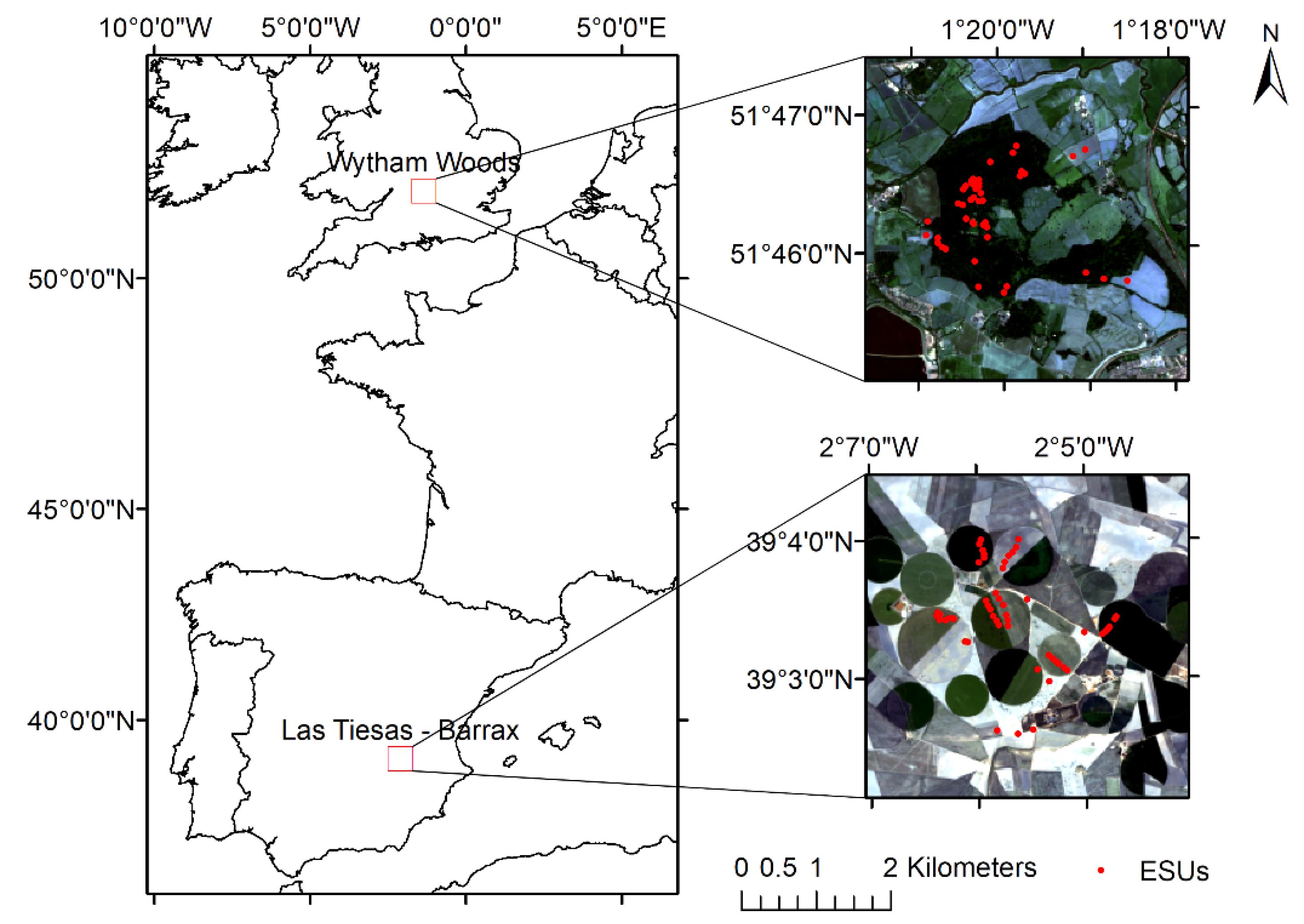
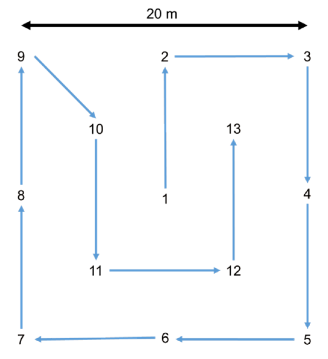
2.1. Study Sites and In Situ Data Collection

Two dedicated field campaigns were conducted in 2018 over study sites representing distinct bio-geophysical characteristics, which were selected on the basis of their representativeness, accessibility, and maturity in terms of previous scientific activities. The first took place between 2 and 8 June 2018 at the Las Tiesas–Barrax experimental farm (39.0549°N, 2.1010°W), which lies approximately 10 km west of Albacete, Castilla-La-Mancha, Spain. Managed by the Instituto Técnico Agronómico Provincial (ITAP), the site is comprised of irrigated crops including alfalfa (Medicago sativa), garlic (Allium sativum), rapeseed (Brassica napus), onion (Allium cepa), sunflower (Helianthus annuus), poppy (Papaver somniferum), and wheat (Triticum aestivum) (Figure 2). The second campaign was conducted between 3 and 12 July 2018 at Wytham Woods (51.7734°N, 1.3384°W), which is located approximately 5 km west of Oxford, Oxfordshire, United Kingdom. As a long-term research forest managed by the University of Oxford, the site consists of ancient seminatural woodland, with oak (Quercus robur), ash (Fraxinus excelsior), beech (Fagus sylvatica), hazel (Corylus avellana), and sycamore (Acer pseudoplatanus) being the dominant species (Figure 2).
In each campaign, in situ reference measurements were conducted within elementary sampling units (ESUs) of approximately 20 m × 20 m (Table 1). Each ESU contained 13 to 15 sampling locations (Figure 3). FAPAR was approximated as the instantaneous black-sky fraction of intercepted photosynthetically active radiation (FIPAR) at 10:30 local solar time, and was derived from estimates of gap fraction obtained using digital hemispherical photography (DHP). Due to the strong absorption by photosynthetic pigments in the PAR domain, previous work has shown the difference between FIPAR and FAPAR to be minimal [10,29,30,31].
DHP images were obtained using a Canon EOS 6D digital single lens reflex (DSLR) camera equipped with a Sigma 8mm F3.5 EX DG fisheye lens, and were processed using CAN-EYE V6.49 [32]. At Las Tiesas–Barrax, downwards-facing images were acquired over the crop canopy, whilst both upwards- and downwards-facing images were acquired at Wytham Woods to characterise the understory and overstory layers. Following Demarez et al. [33], automatic exposure was adopted. To determine gap fraction, for downwards-facing images, the operator was masked from analysis before CAN-EYE’s interactive classification was used to distinguish between green vegetation and the underlying soil background. For upwards-facing images, large tree trunks were masked to minimise the influence of woody material, and the interactive classification was then used to distinguish between the vegetation canopy and the sky.
CCC was determined as the product of leaf chlorophyll concentration (LCC) and leaf area index (LAI). As with FIPAR, LAI was obtained using DHP; in this case, the mean of two solutions provided by CAN-EYE (V5.1 and V6.1) was calculated, following Fuster et al. [15]. LCC was determined using a Konica Minolta SPAD-502 chlorophyll meter, which provides relative values based on the ratio of incident and transmitted radiation at 650 nm and 940 nm. At each sampling location, three leaves were removed from the canopy. At Las Tiesas–Barrax, where all layers were accessible, these leaves were sampled from the top, middle, and bottom of the canopy, enabling vertical variations in LCC to be accounted for. At Wytham Woods, where the top of the canopy was not accessible, leaves were sampled from the middle and bottom of the tree crowns. Six replicate measurements were carried out on each leaf, taking care to avoid major veins, which can lead to inaccurate values [34,35]. ESUs characterised by bare soil were assigned FIPAR and CCC values of zero.
The relative values provided by the SPAD-502 were converted to absolute units using calibration functions specific to each vegetation type. For the Wytham Woods campaign, dedicated calibration data were obtained. This involved the collection of 60 leaves for each species, spanning a range of LCC (assessed visually in terms of leaf colour). Using a 6 mm diameter cork borer, a disc was removed from each leaf, and the mean of three SPAD-502 measurements was calculated. The disc was then placed in 5 mL of dimethyl-sulphoxide (DMSO), administered using a calibrated bottle-top dispenser with adjustable dosing, before being placed in a drying oven at 65 °C overnight to facilitate extraction. Once all chlorophyll was extracted (indicated by the discs being white in colour), a 3 mL aliquot was transferred to a 10 mm path length polystyrene cuvette using a transfer pipette. The absorbance of the sample was then determined at 665 nm and 649 nm using a ThermoFisher Genesys 50 UV-Vis spectrophotometer. From absorbance measured spectrophotometrically, the concentrations of chlorophyll-a and -b were determined in µg mL−1 according to Wellburn [36] as
C a = 12.19   A b s 665 3.45   A b s 649
C b = 21.99   A b s 649 5.32   A b s 665
where A b s 665 and A b s 649 are the absorbance values at 665 nm and 649 nm, respectively.
For the Las Tiesas–Barrax campaign, a comparable procedure was followed using calibration data collected during a previous campaign over a similar site, in which 105 leaves were collected from a range of different crops [37]. For each leaf, two discs were removed using a copper cylinder, and the mean of six SPAD-502 measurements was determined. In this case, the leaf discs were extracted in acetone, and the concentrations of chlorophyll-a and -b in µg mL−1 were determined spectrophotometrically according to Lichtenthaler [38], such that
C a = 11.24   A b s 661.6 2.04   A b s 644.8
C b = 20.13   A b s 644.8 4.19   A b s 661.6
where A b s 661.6 and A b s 644.8 are the absorbance values at 661.6 nm and 644.8 nm, respectively. For both campaigns, once the concentrations of chlorophyll-a and -b were derived, spectrophotometrically-determined LCC was calculated on a mass per unit area basis (in g m−2) as
L C C s p e c = ( C a + C b )   V A
where V is the volume of solvent in which the leaf disc was extracted, and A is the area of the leaf disc.
Calibration functions relating SPAD-502 values to spectrophotometrically-determined LCC were derived using orthogonal distance regression (ODR). Unlike other regression approaches, ODR makes use of uncertainties in predictor and response variables, minimising the sum of squared orthogonal distances between each data point and the model [39]. Thus, the measurement uncertainties associated with each data point are used to inform the model fit. The calibration functions (which are reported in Table A1 of Appendix A) took an exponential form:
L C C S P A D = a   e b   M
where a and b are regression coefficients determined by ODR, and M is the SPAD-502 value.

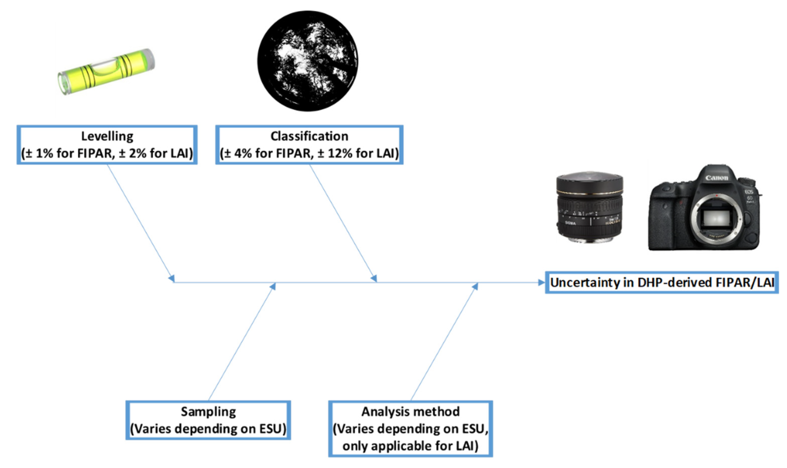
2.2. Quantification of In Situ FIPAR Measurement Uncertainties

Three uncertainty components were considered to estimate the uncertainty associated with in situ FIPAR measurements: levelling, image classification, and sampling (Figure 4). The standard uncertainty due to levelling was assessed using ‘Type B’ evaluation: Origo et al. [40] report a relative standard uncertainty in gap fraction of approximately 1% due to acquiring DHP images by hand as opposed to tripod levelling. The remaining uncertainty components were assessed using ‘Type A’ evaluation. In the case of image classification, a subset of 16 ESUs were classified by three different operators to assess how the decisions made by the operator influenced estimated gap fraction, resulting in a relative standard uncertainty of 4% for FIPAR. Finally, the standard uncertainty due to sampling was assessed for each ESU on the basis of variability in gap fraction. Variability was considered at two distinct scales:
  • Within-image (i.e., the standard error of the mean gap fraction in each zenith ring, over all azimuth cells within an image);
  • Between-image (i.e., the standard error of the mean gap fraction in each zenith ring, over all images).
The two terms were then added in quadrature, such that
u s a m p ( F I P A R ) = ( 1 n j = 1 n σ x ¯ [ P ( θ i ) w i t h i n ] j 2 ) 2 + σ x ¯ [ P ( θ i ) b e t w e e n ] 2
where σ x ¯ [ P ( θ i ) w i t h i n ] and σ x ¯ [ P ( θ i ) b e t w e e n ] represent within- and between-image variability in gap fraction (quantified as the standard error of the mean, denoted σ x ¯ ). The gap fraction in zenith ring i , with a central zenith angle of θ , is denoted P ( θ i ) , whilst j represents the image in question.
To obtain the combined standard uncertainty in FIPAR, all considered components were added in quadrature, such that
u ( F I P A R ) = u l e v e l ( F I P A R ) 2 + u c l a s s ( F I P A R ) 2 + u s a m p ( F I P A R ) 2
where u l e v e l ( F I P A R ) , u c l a s s ( F I P A R ) , and u s a m p ( F I P A R ) are the standard uncertainties in FIPAR due to instrument levelling, image classification, and sampling, respectively. At Wytham Woods, measurements using upwards- and downwards-facing DHP were used to characterise the overstory and understory vegetation, such that
F I P A R t o t a l = F I P A R u p + ( 1 F I P A R u p )   F I P A R d o w n
u ( F I P A R t o t a l ) = [ ( 1 F I P A R u p )   u ( F I P A R d o w n ) ] 2 + [ ( 1 F I P A R d o w n )   u ( F I P A R u p ) ] 2
where F I P A R u p and F I P A R d o w n are the FIPAR values derived using upwards- and downwards-facing DHP, whilst u ( F I P A R u p ) and u ( F I P A R d o w n ) are their respective standard uncertainties as determined according to Equation (8).

2.3. Quantification of In Situ CCC Measurement Uncertainties

As the product of LAI and LCC, the uncertainty associated with in situ measurements of CCC was determined as
u ( C C C ) = [ L C C   u ( L A I ) ] 2 + [ L A I   u ( L C C ) ] 2
where u ( L A I ) and u ( L C C ) are the standard uncertainties in LAI and LCC, respectively. The calculation of these two uncertainty components is described in Section 2.3.1 and Section 2.3.2.

2.3.1. LAI Uncertainty Estimation

To estimate the uncertainty associated with in situ LAI measurements, four uncertainty components were considered: levelling, image classification, sampling, and differences between analysis methods (Figure 4). As for FIPAR, the standard uncertainty due to levelling was assessed using ‘Type B’ evaluation: in the case of LAI, Origo et al. [40] report a relative standard uncertainty of approximately 2%. Again, the remaining uncertainty components were assessed using ‘Type A’ evaluation. For image classification, the operator-influence experiments described in Section 2.2 resulted in a relative standard uncertainty in LAI of 12%. As for FIPAR, the standard uncertainty due to sampling was assessed on the basis of variability in gap fraction (Section 2.2). Finally, the standard uncertainty due to differences between analysis methods was determined as the standard error of the mean of the V5.1 and V6.1 solutions.
Unfortunately, propagating the standard uncertainties in gap fraction due to sampling through the look-up-table inversion approaches used by CAN-EYE to estimate LAI is not straightforward. Therefore, an estimate of the standard uncertainty in LAI due to sampling was determined by propagating the standard uncertainties in gap fraction values through the Warren-Wilson method [41], making use of Lang and Yueqin’s approach [42] to account for foliage clumping, such that
u s a m p ( L A I ) = σ x ¯ [ ln P ( θ 57.5 ° ) ] 0.93
where σ x ¯ [ ln P ( θ 57.5 ° ) ] is the variability in the natural logarithm of gap fraction values at 57.5°, determined as in Equation (7). Note that the V6.1 solution provided by CAN-EYE is constrained to provide results close to those obtained using Warren-Wilson’s method [32], meaning that the resulting standard uncertainties are likely of a similar magnitude to those associated with CAN-EYE’s look-up-table inversion approaches, and represent a good first-order approximation.
To obtain the combined standard uncertainty in LAI, all considered components were added in quadrature, such that
u ( L A I ) = u l e v e l ( L A I ) 2 + u c l a s s ( L A I ) 2 + u s a m p ( L A I ) 2 + u m e t h o d ( L A I ) 2
where u l e v e l ( L A I ) ,   u c l a s s ( L A I ) , u s a m p ( L A I ) , and u m e t h o d ( L A I ) are the standard uncertainties in LAI due to instrument levelling, image classification, sampling, and differences between analysis methods, respectively. At Wytham Woods, LAI was derived as the sum of the understory and overstory components (as obtained using upwards- and downwards-facing DHP). In this case, the standard uncertainty in total LAI was calculated as
u ( L A I t o t a l ) = u ( L A I u p ) 2 + u ( L A I d o w n ) 2
where u ( L A I u p ) and u ( L A I d o w n ) are the standard uncertainties in LAI derived using upwards- and downwards-facing DHP, respectively, as determined according to Equation (13).

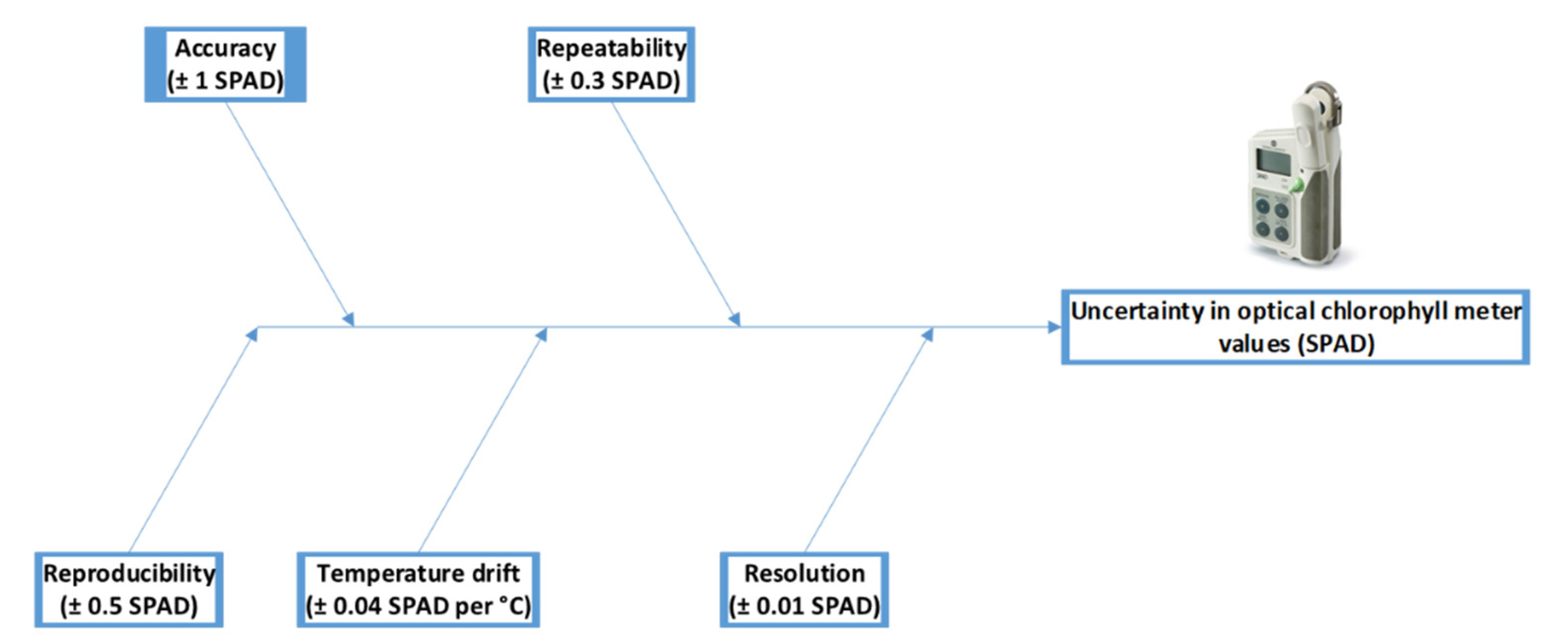
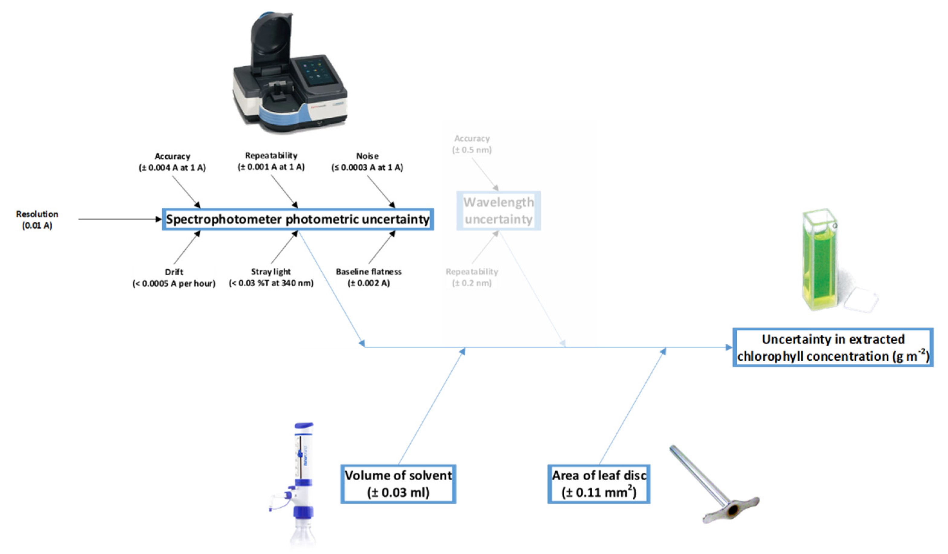
2.3.2. LCC Uncertainty Estimation

In terms of individual in situ LCC measurements, two sources of uncertainty must be considered: those inherent to the SPAD-502, and those related to the calibration function. The uncertainties inherent to the SPAD-502 are easily assessed using ‘Type B’ evaluation, and include accuracy, repeatability, reproducibility, temperature drift, and resolution (Figure 5) [43]. As such, the standard uncertainty in SPAD-502 values was determined as
u ( M ) = u a c c ( M ) 2 + u r e p ( M ) 2 + u r e p r o ( M ) 2 + u t e m p ( M ) 2 + u r e s ( M ) 2
where u a c c ( M ) , u r e p ( M ) , u r e p r o ( M ) , u t e m p ( M ) , and u r e s ( M ) are the standard uncertainties in SPAD-502 values due to accuracy, repeatability, reproducibility, temperature drift, and resolution, respectively.
On the other hand, the uncertainties related to the calibration function are dependent on the uncertainties inherent to the SPAD-502, in addition to those associated with the instruments and apparatus used to determine LCC spectrophotometrically. These include various uncertainty sources related to the spectrophotometer (i.e., photometric accuracy, repeatability, noise, drift, stray light, baseline flatness, and resolution) [44,45], in addition to the volume of extraction solvent released by the dispenser [46], and the area of the leaf disc extracted by the cork borer (Figure 6). These uncertainties can also be assessed using ‘Type B’ evaluation [45,46], with the exception of the latter term, which we assessed by removing discs from a subset of 60 leaves, measuring their area using a flatbed scanner, and determining the standard error of the mean.
It is worth noting that some terms, such as photometric accuracy, noise, and stray light, are dependent on the measured absorbance itself. For these terms, the corresponding uncertainty was determined by linearly interpolating between specifications provided by the manufacturer at different absorbance values. An additional source of uncertainty is related to the accuracy and repeatability of wavelength selection. Experiments in which the measured wavelength was adjusted by ±1 nm were carried out over a range of samples to assess the influence of these components. As the resulting error in absorbance was found to lie within the overall photometric uncertainty, these wavelength related components were not considered further.
Taking into account all the uncertainty sources related to the spectrophotometer, the standard uncertainty in absorbance measured at a given wavelength was obtained as
u ( A b s λ ) = u a c c ( A b s λ ) 2 + u r e p ( A b s λ ) 2 + u n o i s e ( A b s λ ) 2 + u d r i f t ( A b s λ ) 2 + u s t r a y ( A b s λ ) 2 + u f l a t ( A b s λ ) 2 + u r e s ( A b s λ ) 2
where u a c c ( A b s λ ) , u r e p ( A b s λ ) , u n o i s e ( A b s λ ) , u d r i f t ( A b s λ ) , u s t r a y ( A b s λ ) , u f l a t ( A b s λ ) , and u r e s ( A b s λ ) are the standard uncertainties in absorbance at wavelength λ due to photometric accuracy, repeatability, noise, drift, stray light, baseline flatness, and resolution, respectively [44]. By propagating the uncertainties in absorbance values through the spectrophotometric equations described in Section 2.1, we could then obtain the standard uncertainties in chlorophyll-a and -b concentrations. For example, using the equations of Wellburn [36] for DMSO Equations (1) and (2), the standard uncertainties were determined as
u ( C a ) = [ 12.19   u ( A b s 665 ) ] 2 + [ 3.45   u ( A b s 649 ) ] 2
u ( C b ) = [ 21.99   u ( A b s 649 ) ] 2 + [ 5.32   u ( A b s 665 ) ] 2
where u ( A b s 665 ) and u ( A b s 649 ) are the standard uncertainties in absorbance at 665 nm and 649 nm, respectively. Finally, the combined standard uncertainty in spectrophotometrically-determined LCC on a mass per unit area basis was derived as
u ( L C C s p e c ) = [ V A   u ( C a ) ] 2 + [ V A   u ( C b ) ] 2 + [ C a + C b A   u ( A ) ] 2 + [ V   ( C a + C b ) A 2   u ( V ) ] 2
where u ( V ) and u ( A ) are the uncertainties in the volume of solvent dispensed and area of the leaf disc, respectively.
As described in Section 2.1, calibration functions were derived using ODR [39], in which the uncertainties in both SPAD-502 values and spectrophotometrically-derived LCC were used to inform the model fit. To determine the standard uncertainty associated with calibrated LCC values, the uncertainties in both the SPAD-502 values and calibration coefficients were propagated through the calibration function Equation (6). Correlation was accounted for, such that
u ( L C C S P A D ) = [ e b   M   u ( a ) ] 2 + [ a   M   e b   M   u ( b ) ] 2 + [ a   b   e b   M   u ( M ) ] 2 + 2 [ e b   M   a   b   e b   M   u ( a , b ) + e b   M   a   M   e b   M   u ( a ,   M ) + a   b   e b   M   a   M   e b   M   u ( M , b ) ]
where u ( a ) and u ( b ) are the standard uncertainties of the calibration coefficients provided by ODR, and u ( a ,   M ) , u ( a , b ) , and u ( M , b ) are covariance terms.
Because the mean of multiple in situ measurements was taken to represent each ESU, the uncertainties associated with each individual observation were finally propagated through the calculation of the mean, whilst the standard error of the mean was calculated to reflect uncertainty due to sampling. Thus, the combined standard uncertainty in SPAD-derived LCC at the ESU level was determined by adding these two terms in quadrature, such that
u ( L C C ) = [ 1 n i = 1 n u ( L C C S P A D i ) 2 ] 2 + σ x ¯ ( L C C S P A D ) 2
where σ x ¯ ( L C C S P A D ) is the standard error of the mean of LCC observations within the ESU.

2.4. Estimation of Uncertinaites in High-Spatial-Resolution Imagery

Sentinel-2 Multispectral Instrument (MSI) imagery acquired within one week of in situ data collection was used for the purposes of upscaling in situ reference measurements. MSI provides data in 13 spectral bands at visible, near-infrared, and shortwave-infrared wavelengths, including three bands positioned in and around the red-edge, making it well-suited to upscaling FIPAR and CCC data. Currently, per-pixel uncertainties are not provided within MSI L1C or L2A products. However, the Sentinel-2 Radiometric Uncertainty Tool (RUT) developed by Gorroño et al. [47] enables per-pixel uncertainties to be estimated for L1C top-of-atmosphere reflectance products. Whilst such a tool is not yet available for L2A bottom-of-atmosphere reflectance products, because our upscaling approach is based on an empirical transfer function using a single image and the atmospheric conditions could be considered constant over the 5 km x 5 km study site extent, atmospheric correction was not mandatory [17,28]. The RUT currently incorporates the following uncertainty components, which are combined in accordance with the GUM [47]:
  • Instrument noise (shot, thermal etc. noise introduced by the detectors);
  • Out-of-field straylight systematic (telescope out-of-field light that results in a positive bias)*;
  • Out-of-field straylight random (telescope out-of-field light that results in a random spatial dispersion);
  • Crosstalk (focal plane (optical) and front-end electronics (electrical) interband signal);
  • Analogue-to-digital conversion quantisation (at MSI’s video chain unit);
  • Dark signal stability (residual thermal fluctuations of the detector offset along the orbit)*;
  • Gamma knowledge (knowledge on the correction for nonlinearity and nonuniformity);
  • Diffuser absolute knowledge (knowledge on the diffuser reflectance factor)*;
  • Diffuser temporal knowledge (estimated effect of diffuser degradation)*;
  • Diffuser cosine effect (cosine correction knowledge as a consequence of angular noise)*;
  • Diffuser straylight residual (residual of the correction of the stray-light during in-flight diffuser calibration)*;
  • L1C image quantisation (effect of the finite resolution of the L1C reflectance factor).
For consistency with the extent of the sampled ESUs, and to take advantage of MSI’s red-edge bands, L1C top-of-atmosphere reflectance values were aggregated to a common 20 m spatial resolution using mean value downsampling. However, mean value downsampling cannot be used to correctly propagate the per-pixel uncertainties provided by the RUT through the aggregation procedure, since several uncertainty components (marked with * above) are considered to be correlated in space. Instead, the ‘select/deselect’ approach described by Gorroño et al. [48] was adopted. This involved running the RUT twice, enabling the uncertainty components that are uncorrelated in space to be separated from those that are correlated in space. The standard uncertainty in the aggregated pixel values was then taken as the mean of the two RUT outputs [48].

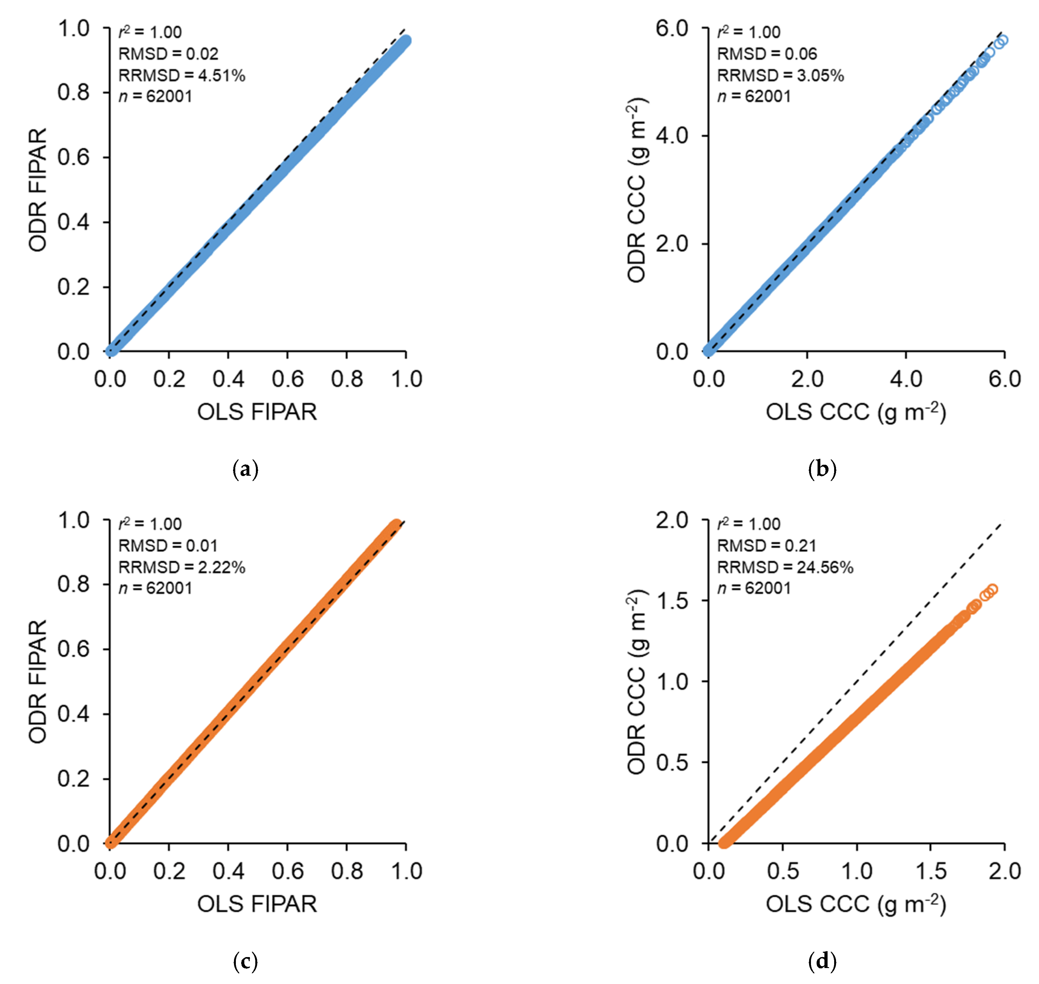
2.5. Derivation of Transfer Functions Accounting for Uncertainties and Production of High-Spatial-Resolution Reference Maps with Per-Pixel Uncertainty Estimates

To enable uncertainties associated with the in situ reference measurements and high-spatial-resolution imagery to be used by the fitting procedure, as with the SPAD-502 calibration functions, ODR was used to derive transfer functions for upscaling [39]. Transfer functions were established between in situ reference measurements and one of three vegetation indices (depending on the study site and bio-geophysical variable). For FIPAR, the normalised difference vegetation index (NDVI) [49] was used for both campaigns as a result of its known near-linear association [50]. For CCC, the Sentinel-2 Terrestrial Chlorophyll Index (S2TCI) [51,52] was used for the Las Tiesas–Barrax campaign, whilst the Inverted Red Edge Chlorophyll Index (IRECI) [51] was found to provide better performance for the Wytham Woods campaign. The NDVI, S2TCI and IRECI were calculated as
N D V I = B 8 B 4 B 8 + B 4
S 2 T C I = B 6 B 5 B 5 B 4
I R E C I = B 7 B 4 B 5 / B 6
where B 8 , B 7 , B 6 , B 5 , and B 4 are top-of-atmosphere reflectance values in MSI bands centred at 842 nm, 783 nm, 740 nm, 705 nm and 665 nm, respectively. Standard uncertainties were determined as
u ( N D V I ) = [ 2   B 4 ( B 8 + B 4 ) 2   u ( B 8 ) ] 2 + [ 2   B 8 ( B 8 + B 4 ) 2   u ( B 4 ) ] 2
u ( S 2 T C I ) = [ 1 B 5 B 4   u ( B 6 ) ] 2 + [ B 4 B 6 ( B 5 B 4 ) 2   u ( B 5 ) ] 2 + [ B 6 B 5 ( B 5 B 4 ) 2   u ( B 4 ) ] 2
u ( I R E C I ) = [ B 6 B 5   u ( B 7 ) ] 2 + [ B 6 B 5   u ( B 4 ) ] 2 + [ B 6   ( B 4 B 7 ) B 5 2   u ( B 5 ) ] 2 + [ B 7 B 4 B 5   u ( B 6 ) ] 2
where u ( B 8 ) , u ( B 7 ) , u ( B 6 ) , u ( B 5 ) , and u ( B 4 ) are the standard uncertainties in top-of-atmosphere reflectance values provided by the RUT for MSI bands centred at 842 nm, 783 nm, 740 nm, 705 nm and 665 nm, respectively. Note that for the Las Tiesas–Barrax campaign, seven alfalfa ESUs were excluded from the derivation of the transfer functions because the crop had been thinned prior to the MSI acquisition, but after the in situ measurements were made.
Once fit, the transfer functions were used to derive high-spatial-resolution reference maps of FIPAR and CCC over the 5 km × 5 km extent of each study site. Since linear transfer functions were adopted, FIPAR and CCC were derived as
y = a   x + b
where x is the associated vegetation index, and a and b are the regression coefficients provided by ODR. An analysis to verify that linear transfer functions were the most appropriate is presented in Appendix B. Accounting for correlation, per-pixel uncertainties were derived as
u ( y ) = [ x   u ( a ) ] 2 + [ a   u ( x ) ] 2 + u ( b ) 2 + 2 [ x   a   u ( a ,   x ) + x   u ( a , b ) + a   u ( x , b ) ]
where u ( a ) and u ( b ) are the standard uncertainties of regression coefficients provided by ODR, u ( x ) is the standard uncertainty in the vegetation index as determined in Equations (25)–(27), and u ( a , x ) , u ( a , b ) , and u ( x , b ) are covariance terms.
Following CEOS WGCV LPV good practices [16], in addition to the derived FIPAR and CCC values and their uncertainties, a categorical quality flag layer was produced to identify areas in which the transfer function was acting as an extrapolator (and therefore might provide less reliable outputs). This was achieved by identifying pixels lying within the multispectral convex hull of the sampled ESUs, following the approach of Martinez et al. [28]. Both ‘strict’ and ‘large’ convex hulls were defined (the latter by assuming 5% noise in the high-spatial-resolution imagery). Pixels within the ‘strict’ convex hull were not subject to extrapolation and could be categorised as high confidence. Pixels lying outside of the ‘strict’ convex hull, but within the ‘large’ convex hull could be categorised as good confidence. Pixels lying outside of the ‘large’ convex hull represented extrapolation and were categorised as low confidence.
The derived high-spatial-resolution reference maps were primarily evaluated using leave-one-out cross validation. Overall agreement was quantified in terms of the coefficient of determination (r2), root mean square error (RMSE), and relative RMSE (RRMSE), the latter of which was computed by dividing the RMSE by the mean of the reference values. To benchmark our ODR-based upscaling approach against current state-of-the-art techniques, we also derived transfer functions and high-spatial-resolution reference maps using ordinary least squares (OLS) and IRLS regression. As a robust regression procedure, IRLS has been previously used by the CEOS WGCV LPV community to minimise the influence of outliers in the derivation of transfer functions [28], whilst OLS, which does not consider measurement uncertainties in the predictor or response variables, remains a widely used approach. A pixel-to-pixel comparison of the ODR- and OLS/IRLS-based high-spatial-resolution reference maps was conducted, and agreement was quantified using the r2, root mean square difference (RMSD), and relative RMSD (RRMSD).

3. Results

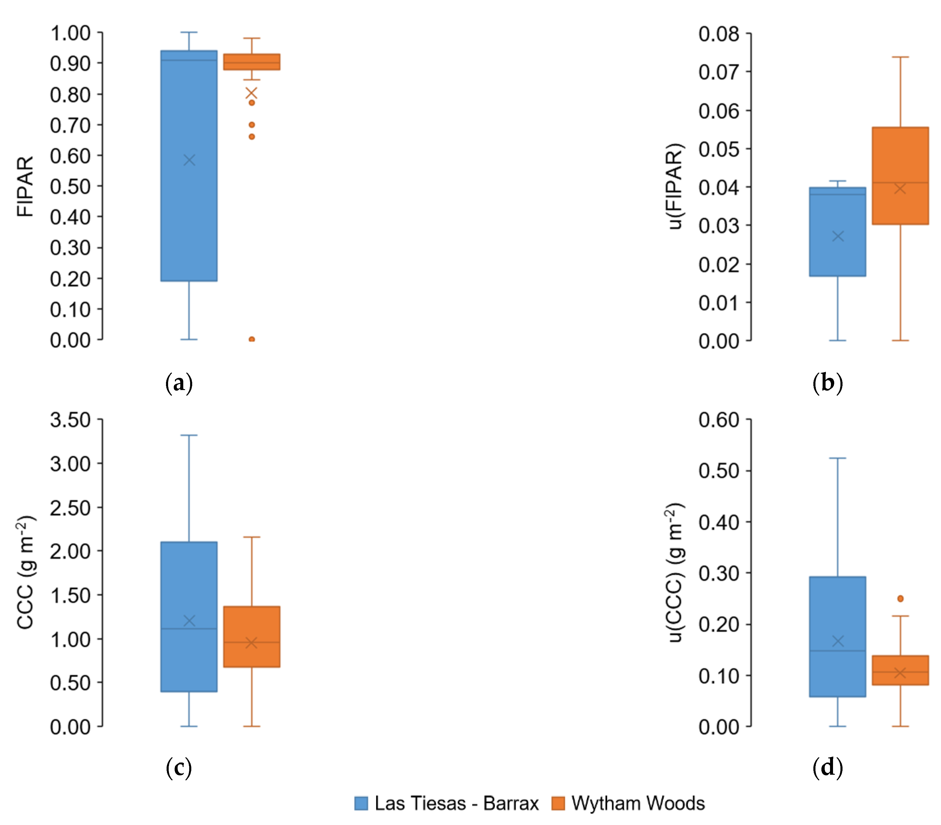
3.1. In Situ Reference Measurements

As a result of their distinct bio-geophysical characteristics, the in situ reference measurements acquired during the FRM4VEG field campaigns varied substantially between the two study sites. In situ FIPAR measurements ranged from 0.00 to 1.00 in the Las Tiesas–Barrax campaign, with a mean of 0.58 and median of 0.91 (Figure 7a). On average, higher FIPAR values were experienced at Wytham Woods, where in situ measurements ranged from 0.00 to 0.98, but with a mean and median of 0.80 and 0.90, respectively (Figure 7a). Considerably less variability was observed in the in situ measurements at Wytham Woods (standard deviation = 0.02) when compared to the Las Tiesas–Barrax campaign (standard deviation = 0.29) (Figure 7a). Average in situ FIPAR measurement uncertainties were comparable in both campaigns (mean and median = 0.04), but were more variable in the Wytham Woods campaign (range = 0.07, standard deviation = 0.02) than at Las Tiesas–Barrax (range = 0.04, standard deviation = 0.01) (Figure 7b).
As expected, an opposite pattern was observed for CCC, with lower average values obtained in the Wytham Woods campaign (mean = 0.95 g m−2, median = 0.96 g m−2) than at Las Tiesas–Barrax (mean = 1.21 g m−2, median = 1.12 g m−2) (Figure 7c). Again, however, in situ CCC measurements were less variable at Wytham Woods (range = 2.16 g m−2, standard deviation = 0.59 g m−2) than in the Las Tiesas–Barrax campaign (range = 3.31 g m−2, standard deviation = 0.96 g m−2) (Figure 7c). In contrast to FIPAR, higher and more variable in situ CCC measurement uncertainties were observed at Las Tiesas–Barrax (mean = 0.17 g m−2, median = 0.15 g m−2, range = 0.52 g m−2, standard deviation = 0.13 g m−2) than in the Wytham Woods campaign (mean = 0.10 g m−2, median = 0.11 g m−2, range = 0.25 g m−2, standard deviation = 0.06 g m−2) (Figure 7d), though the magnitude of the CCC values in each campaign should be borne in mind when interpreting these uncertainties.

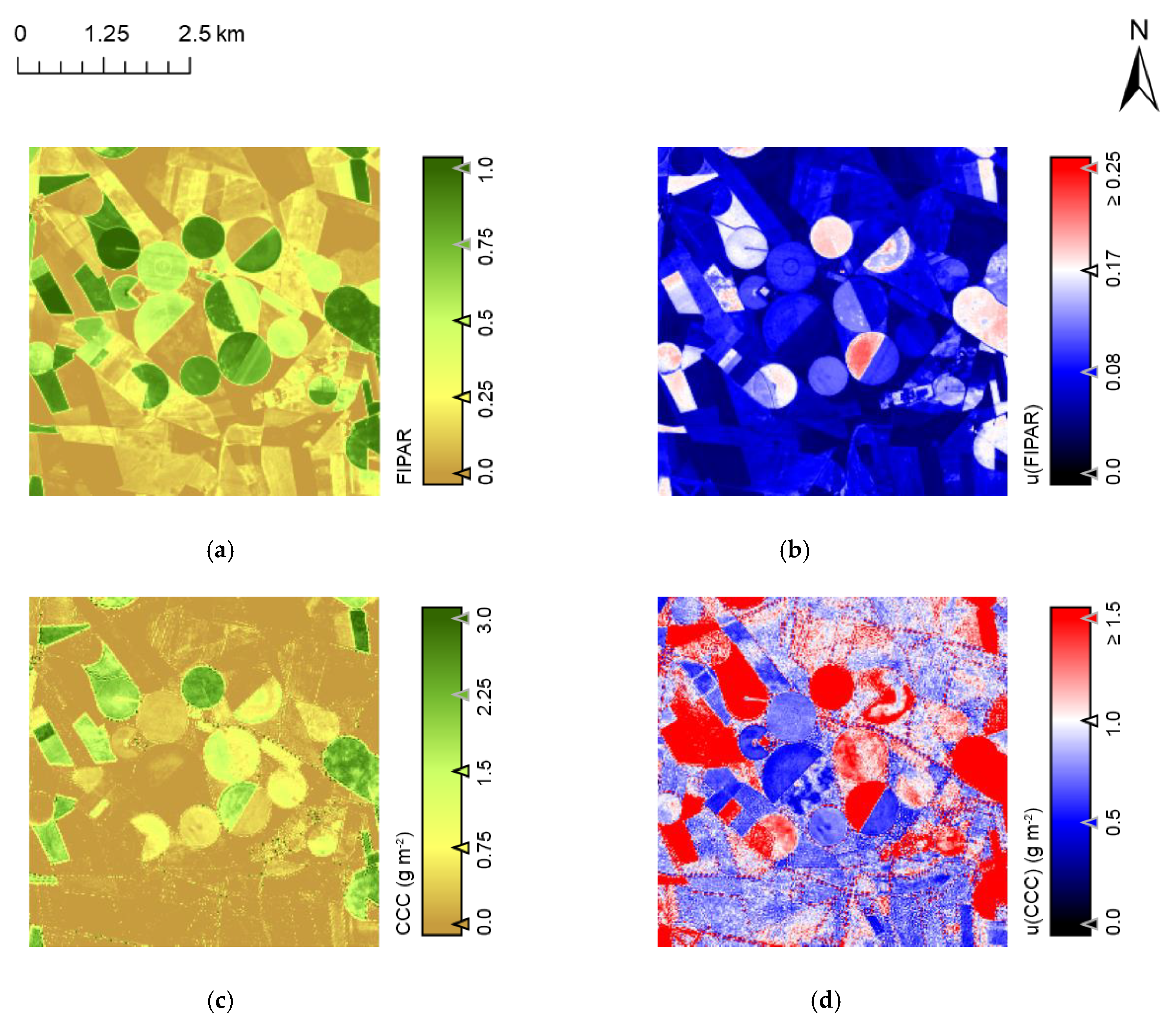
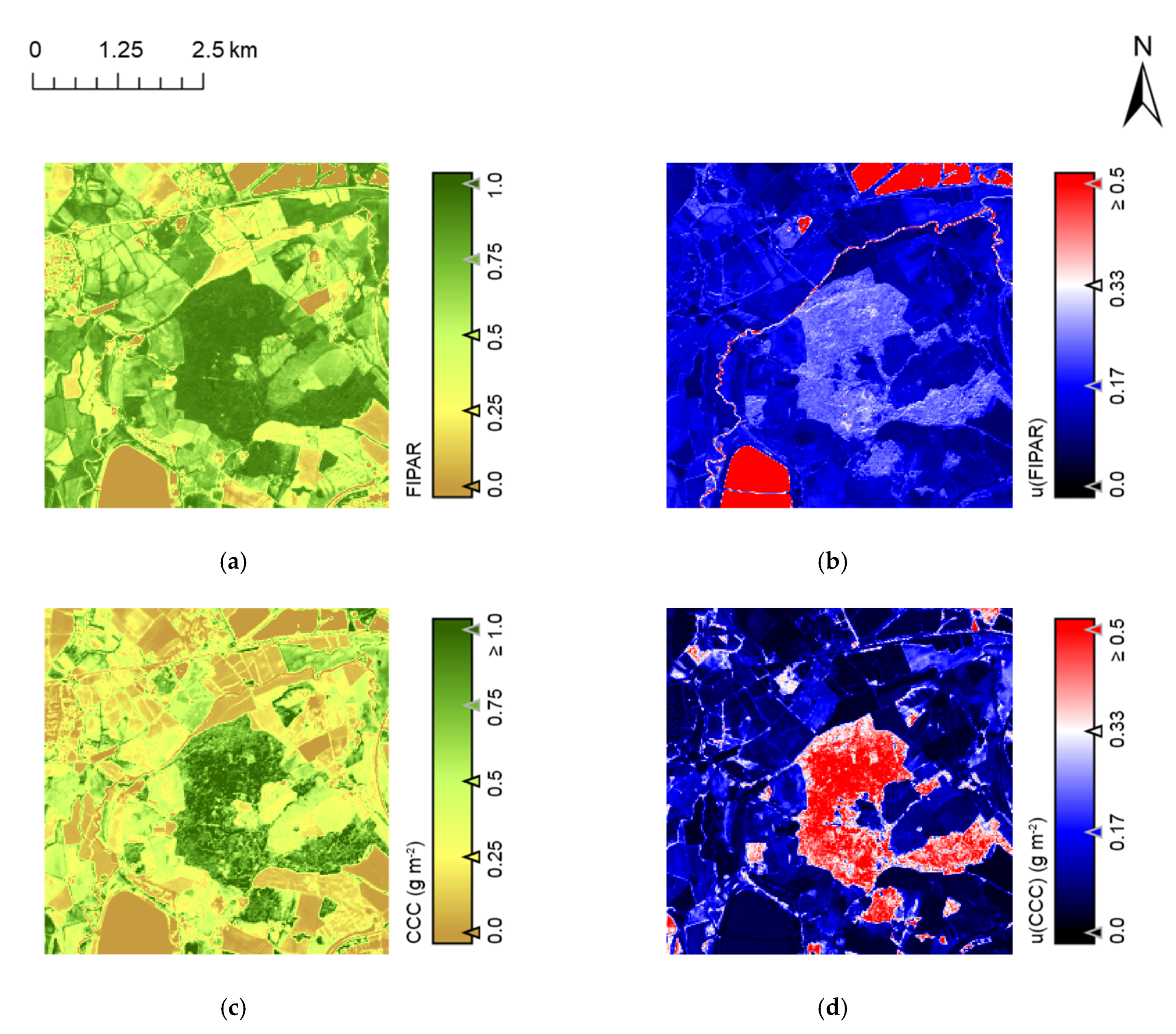
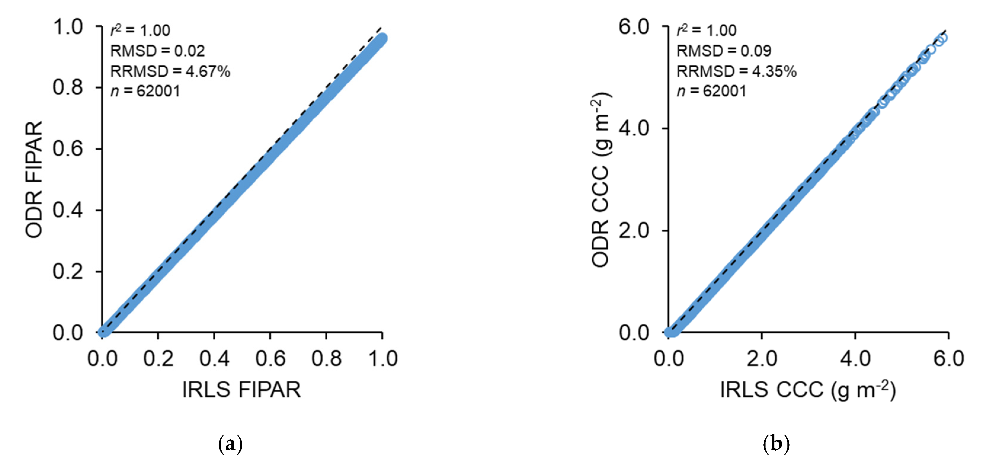
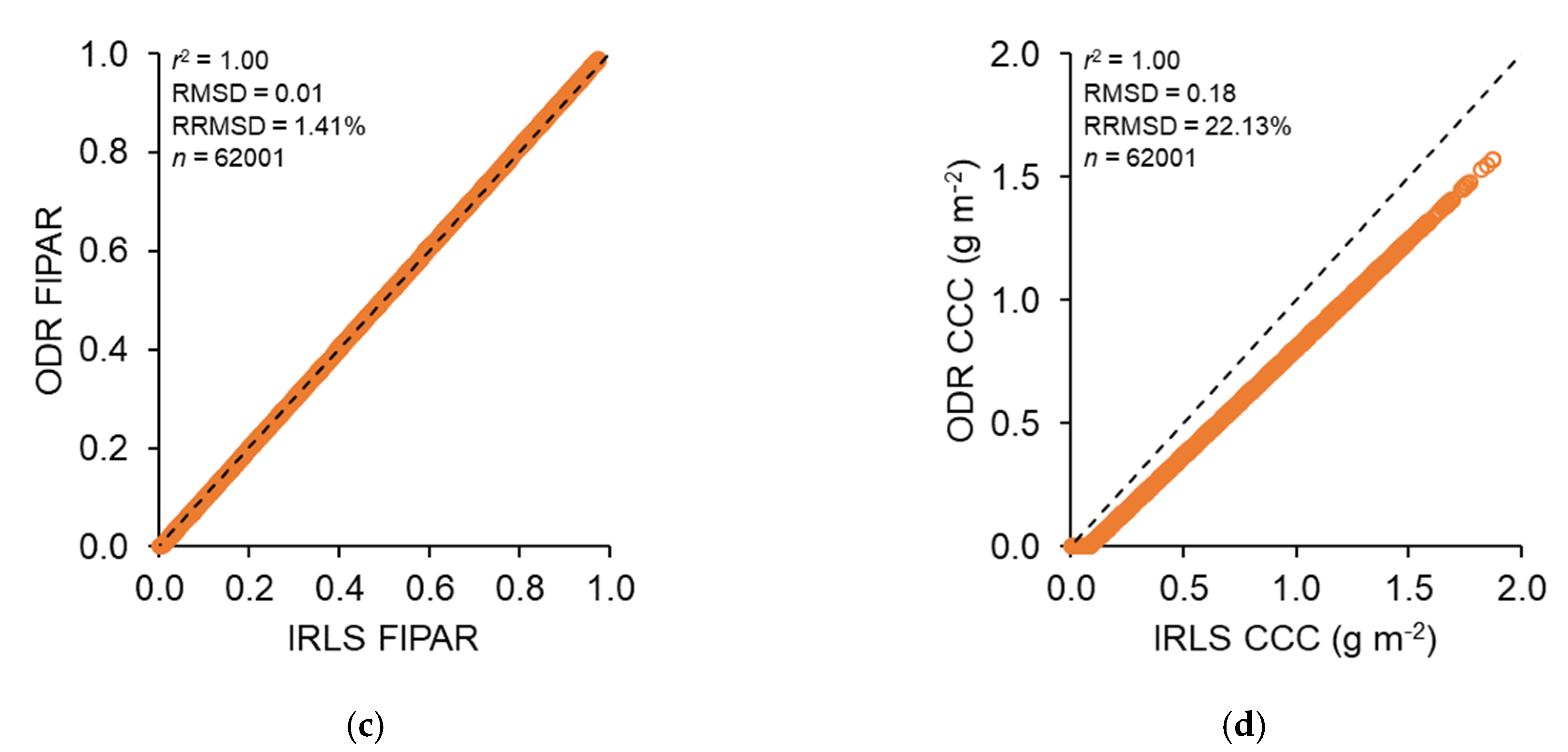
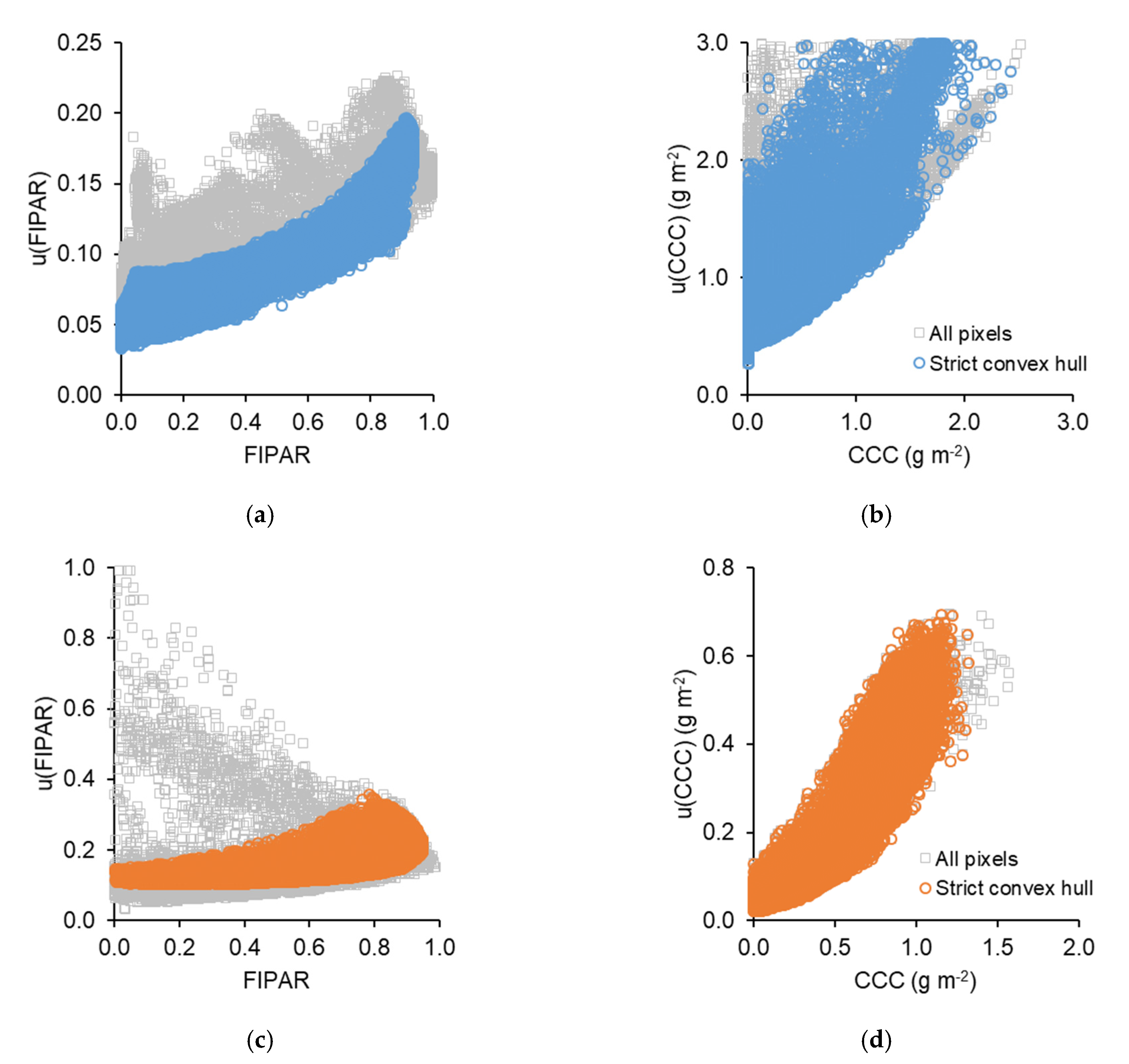
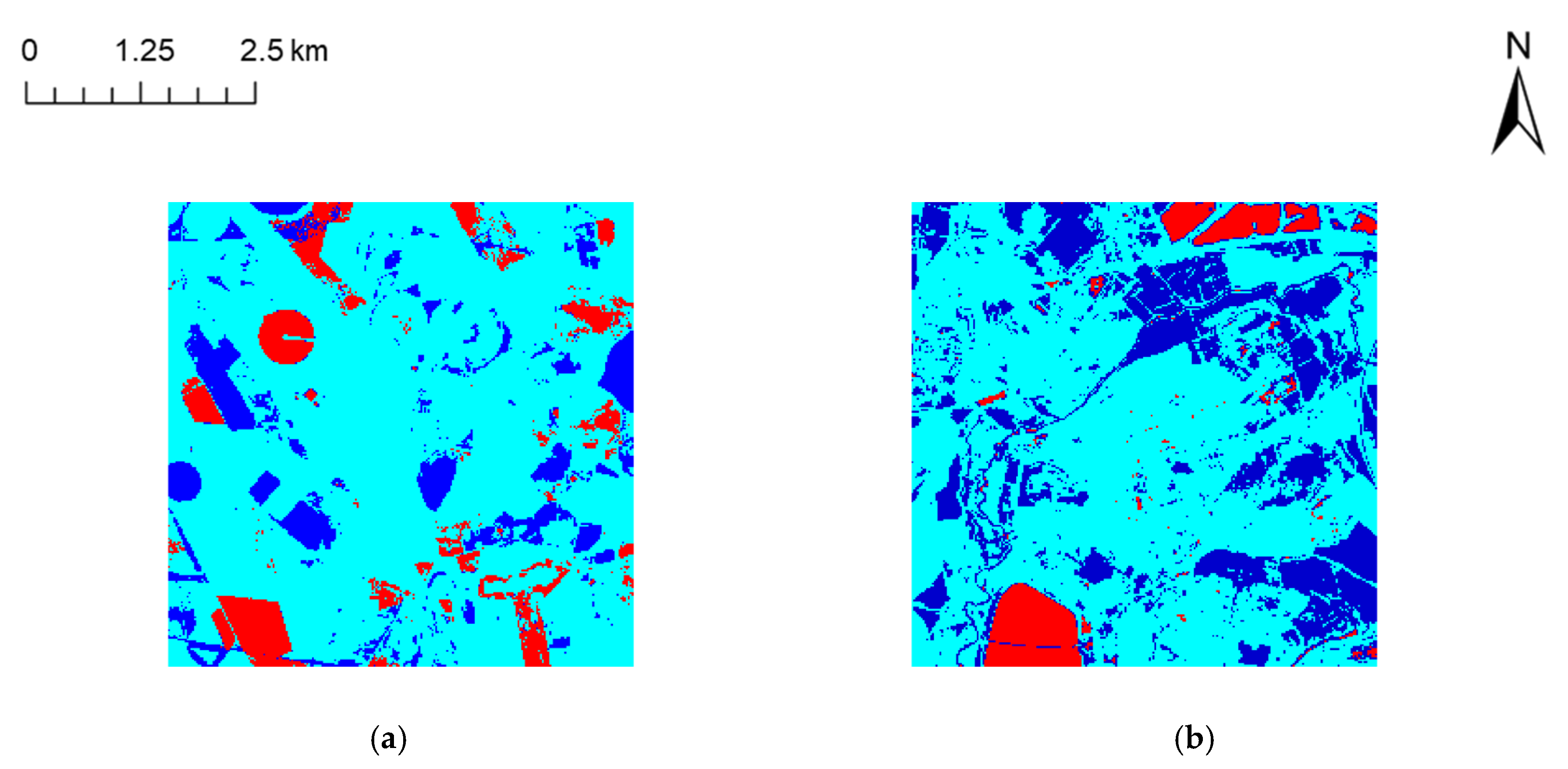
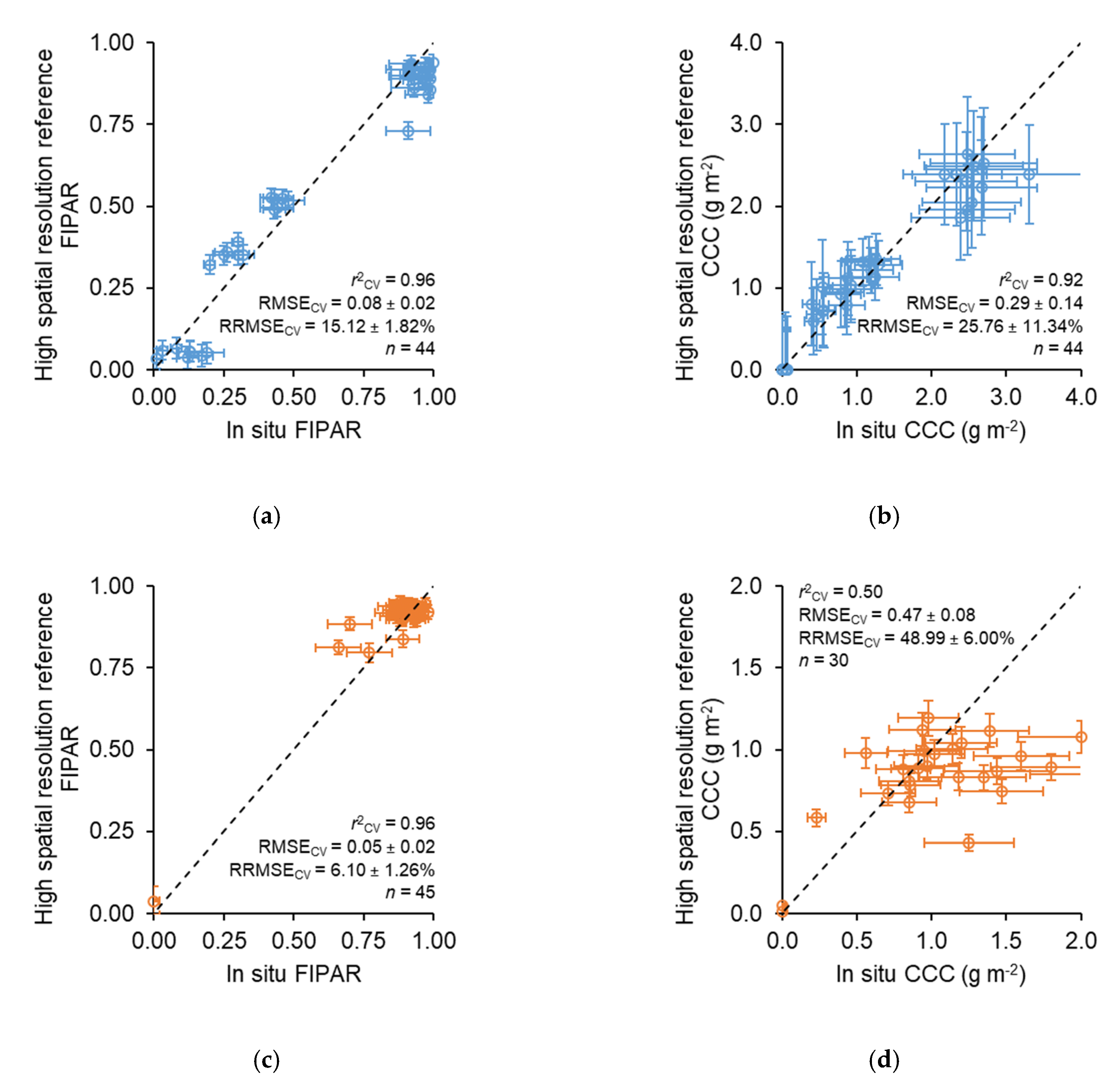
3.2. High-Spatial-Resolution Reference Maps

As with the in situ reference measurements, differences in the range and distribution of FIPAR and CCC values were observed between study sites in the derived high-spatial-resolution reference maps, with lower FIPAR and higher CCC values observed at Las Tiesas–Barrax (Figure 8) when compared to the Wytham Woods campaign (Figure 9). From the high-spatial-resolution reference maps over Las Tiesas–Barrax, cropped and bare fields were clearly identifiable, and differences in the condition of vegetation within individual fields were also apparent (Figure 8). These intrafield variations were more clearly distinguished in terms of CCC than FIPAR. Fields demonstrating high FIPAR values were not always characterised by high CCC, highlighting the different (but complementary) information provided by the two bio-geophysical variables. For FIPAR, uncertainties appeared to be predominantly correlated with FIPAR magnitude, whereas for CCC, patterns were less clear (Figure A1 in Appendix C). Whilst the minimum uncertainty associated with a given CCC value increased with CCC magnitude (such that the lower uncertainties occurred only at lower CCC values), higher uncertainties did occur at all CCC magnitudes. We hypothesise that pixels with higher uncertainties at low to mid CCC values represented crop types that were not sampled (and so were not incorporated in the data used to train the transfer functions) (Figure 8). Indeed, for CCC values between 0.0 and 0.5 g m−2, the highest uncertainties were associated with pixels for which the transfer function was acting as an extrapolator according to the convex hull-based quality flag layer (Figure A1 in Appendix C).
At Wytham Woods, the high-spatial-resolution reference maps permitted easy identification of the woodland, which had the highest FIPAR and CCC values, whilst lower values were associated with the surrounding fields and nonvegetated areas (Figure 9). Within the woodland, variations in vegetation condition were more clearly distinguished in terms of CCC than FIPAR. In contrast to the patterns observed at Las Tiesas–Barrax, uncertainties in CCC appeared to be predominantly controlled by CCC magnitude, whereas the greatest uncertainties in FIPAR occurred at low to mid FIPAR values (Figure A2 in Appendix D), representing areas outside of the woodland (Figure 9). Since these areas were not sampled in the field campaign, they were not incorporated in the transfer function’s training data, and as a result uncertainties over these areas would be expected to be higher. Again, the convex hull-based quality flag layer indicated that over the areas with the highest uncertainties in FIPAR, the transfer function was acting as an extrapolator (Appendix C and Appendix D).
The performance of the high-spatial-resolution reference maps, as assessed using leave-one-out cross validation, varied between bio-geophysical variable and study site. The FIPAR reference maps were characterised by the highest r2CV and lowest RRMSECV values (r2CV = 0.96, RRMSECV = 6.10% to 15.12%), indicating the transfer functions were better able to retrieve FIPAR than CCC, for which lower r2CV and higher RRMSECV values were obtained (r2CV = 0.50 to 0.92, RRMSECV = 25.76% to 48.99%) (Figure 10). This reflects the greater relative uncertainties associated with the in situ CCC measurements used to train the transfer functions (Figure 7), which, as the product of LAI and LCC, incorporate numerous additional sources of uncertainty. When combined with uncertainties inherent to the Sentinel-2 MSI imagery, this explains the reduced accuracy for CCC. It is worth noting that because the in situ reference measurements and high-spatial-resolution reference maps were accompanied by uncertainty estimates, the expanded uncertainty (k = 2) of the derived RMSECV and RRMSECV values could also be calculated. As expected, the standard uncertainties within these statistics were highest for CCC (Figure 10).
In terms of the comparison of our upscaling method with the current state-of-the-art, the ODR- and OLS/IRLS-based high-spatial-resolution reference maps of FIPAR demonstrated a high degree of consistency (r2 = 1.00, RMSD = 0.01 to 0.02, RRMSD = 1.41% to 4.67%) (Figure 11 and Figure 12), providing confidence that the approach represents a suitable alternative. Good correspondence was also obtained in the case of CCC (r2 = 1.00, RMSD = 0.06 to 0.21, RRMSD = 3.05% to 24.56%), though with some disagreement at Wytham Woods, where the OLS- and IRLS-based high-spatial-resolution reference maps provided systematically higher CCC values then the ODR-based one (Figure 11 and Figure 12). This reflects the fact that ODR reduces the weight of points with larger measurement uncertainties in the predictor and response variables (Figure 10), whereas IRLS simply reduces the weight of points with larger residuals, regardless of the measurement uncertainty associated with each point. Meanwhile, OLS applies no weighting. It is worth noting that although absolute in situ CCC measurement uncertainties were lower at Wytham Woods than at Las Tiesas–Barrax (Figure 7), relative to the magnitude of the CCC measurements themselves, the uncertainties at Wytham Woods were, in fact, greater. In future work, it may, therefore, be beneficial to derive relative uncertainties, for example by normalising by the magnitude (or mean) of the variable in question.

4. Discussion

4.1. Utility of End-to-End Uncertainty Evaluation for Conformity Testing

Although considerable progress in the validation of vegetation bio-geophysical products has been made over the past two decades, a lack of in situ reference measurement uncertainty quantification has limited our ability to reliably demonstrate compliance with product uncertainty requirements through conformity testing [8], whilst the incorporation of uncertainties within upscaling procedures has remained poorly addressed. Following FRM principles and adopting a metrological approach, we developed an end-to-end uncertainty evaluation framework for quantifying the uncertainties associated with in situ reference measurements of FIPAR and CCC, and incorporating these uncertainties (as well as those associated with high-spatial-resolution imagery) within the upscaling procedure. Importantly, the proposed uncertainty evaluation procedures are equally applicable to other relevant bio-geophysical variables such as leaf area index (LAI), the fraction of vegetation cover (FCOVER), and canopy water content (CWC). By providing high-spatial-resolution reference maps with per-pixel uncertainty estimates, the FRM4VEG procedures will facilitate conformity testing of moderate spatial resolution vegetation bio-geophysical products. Instead of assuming that upscaled in situ reference measurements represent the truth, in future validation exercises, it will be possible to determine a product’s compliance with uncertainty requirements in a robust and traceable manner.
Though the scope of this study was limited to in situ reference measurement uncertainty evaluation, for conformity testing to be most successful, there is also room for advances in the uncertainty evaluation techniques used by the EO products themselves. As recently noted [53], many vegetation bio-geophysical products are now providing some form of uncertainty estimate, but this is often a statistical measure associated with the retrieval scheme (for example, the standard deviation of candidate solutions within a look-up table or as provided by machine learning regression algorithms such as Gaussian process regression) [1,5,6,54]. In contrast, few products adopt a metrological approach explicitly incorporating all relevant terms of the uncertainty budget [55,56,57,58]. In an ideal case, uncertainty estimates accompanying EO products should also be derived in an end-to-end manner, propagating uncertainties associated with L1 radiometry through to L2 atmospheric correction [26] and the subsequent bio-geophysical retrieval scheme.

4.2. Limitations and Potential Refinements

Whilst the uncertainty evaluation framework described in this paper represents an important step towards the metrological treatment of vegetation bio-geophysical product validation, it could be further extended and refined. For example, in terms of quantifying uncertainties for the DHP-derived in situ reference measurements, although several major uncertainty components were considered, other sources of uncertainty (including exposure settings and sub-optimal illumination conditions) were not, meaning that the uncertainties associated with the in situ measurements may be somewhat optimistic. These factors, to which DHP-derived variables are known to be sensitive [33,59,60,61,62,63,64,65], should be investigated in future work. A further source of uncertainty that was not explicitly considered in this study is the difference between FIPAR and FAPAR. Though the difference between these two quantities is typically considered to be minimal [10,29,30,31], Gobron et al. [30] demonstrated that errors of up to 0.1 can occur over very bright backgrounds, whilst Putzenlechner et al. [66] suggest that two-flux FIPAR may overestimate four-flux FAPAR in forest environments. In future work, the uncertainty associated with this assumption should be better quantified and could be incorporated as an additional uncertainty component.
For the in situ reference measurements of LCC at Wytham Woods, the fact that leaves could not be sampled from the top of the tree crowns might also introduce some degree of bias. For example, in a temperate mixed forest, Gara et al. [67] found statistically significant differences in upper and lower canopy LCC during the summer, though these differences were considerably lower than for other investigated leaf traits and were not statistically significant during the spring or autumn. In terms of deciduous broadleaf species, for ash, birch, and elm, Koike et al. [68] found LCC was highest in the middle of the canopy, whereas, for alder and walnut, the greatest LCC values occurred at the top of the canopy, and, for maple and basswood, LCC decreased throughout the vertical profile. The varied nature of these previous findings indicates a need for further investigation, and taking advantage of recently extended monitoring tower, an experiment to assess vertical variations in LCC at Wytham Woods is planned under phase two of FRM4VEG.
In addition to incorporating further uncertainty components, another area where the proposed uncertainty evaluation framework could be improved is in the handling of correlation. Since the correlation between uncertainty terms related to the in situ reference measurements was often unknown, independence was assumed in the majority of uncertainty propagation equations described in this study. In future work, incorporation of the best available knowledge on correlation could be envisaged, even if only to assume terms are fully correlated, partially correlated, or fully uncorrelated, as was done by Gorroño et al. [48]. Furthermore, the uncertainty evaluation procedures developed should be applied to other instruments used for measuring bio-geophysical variables, such as the LI-COR LAI-2200 and Meter Group AccuPar LP-80 devices. Since they operate on similar principles, the methods described in this paper are also applicable to these instruments.
In terms of upscaling, a refinement to the procedure presented in this study would involve the use of L2A bottom-of-atmosphere MSI data as opposed to L1C top-of-atmosphere MSI data, once a L2 RUT is available. Because empirical transfer functions using a single high-spatial-resolution image per campaign were adopted, and because atmospheric conditions could be considered constant over the extent of each site, atmospherically corrected data were not necessary in this study [17,28]. However, if in situ reference measurements and high-spatial-resolution imagery acquired over multiple dates were to be used, atmospheric correction would be required. As an increasing number sites are equipped with permanent, automated instrumentation, this will become an important consideration, since consistent time-series of high-spatial-resolution imagery are needed to upscale the temporally continuous in situ data provided by such systems [69,70]. It is worth noting that the development of a L2 RUT for the Sentinel-2 mission is the subject of a recently initiated ESA-funded project [71].
Having demonstrated the uncertainty evaluation framework over two sites of distinct bio-geophysical characteristics, the next phase of FRM4VEG will focus on refining the procedures developed in phase one, and applying them in additional field campaigns. Using the consolidated data, it should be possible to identify the most common and substantial uncertainty contributors and inform future in situ sampling and measurement protocols accordingly. In addition to further field campaigns, detailed consideration will be given to the use of permanent instrumentation [72,73,74,75,76,77,78,79]. This will include a review of site deployment considerations and an initial plan for the establishment of permanent ESA-supported FRM4VEG ‘supersites’. Finally, to increase the volume of FRM-compliant data available for vegetation bio-geophysical product validation, it is also anticipated that the FRM4VEG uncertainty evaluation procedures will be adopted, where applicable, by other related validation efforts, such as the Copernicus Ground Based Observations for Validation (GBOV) service [9]. Combined, these activities will provide a rich resource of reference data which can be exploited in future validation exercises for product conformity testing.

5. Conclusions

In this study, we developed and applied an end-to-end uncertainty evaluation framework for quantifying the uncertainties associated with FAPAR and CCC reference data. These procedures, which provide high-spatial-resolution reference maps with per-pixel uncertainty estimates, will facilitate conformity testing of moderate spatial resolution vegetation bio-geophysical products. Rather than assuming reference data represent the truth, it will, therefore, be possible to determine a product’s compliance with uncertainty requirements in a robust manner. Having demonstrated the uncertainty evaluation framework in two field campaigns, future work will focus on extending and refining the FRM procedures to incorporate additional sources of uncertainty, applying them to additional sites and bio-geophysical variables, and investigating their applicability to permanent instrumentation in addition to traditional field campaign-based measurements performed under other validation projects and initiatives.

Author Contributions

Conceptualization, L.A.B., F.C., N.O., J.N., V.B. and J.D.; methodology, L.A.B., F.C., V.G.-S., N.O., B.F. and J.S.-Z.; software, L.A.B., F.C., V.G.-S., B.F. and J.S.-Z.; validation, L.A.B., F.C., V.G.-S., B.F. and J.S.-Z. formal analysis, L.A.B., F.C., V.G.-S., B.F. and J.S.-Z.; investigation, L.A.B., F.C., V.G.-S., N.O., B.F., H.M., J.P.-G., J.S.-Z. and V.B.; resources, L.A.B., F.C., N.O., J.N. and J.D.; data curation, L.A.B., F.C., V.G.-S., B.F., J.S.-Z. and J.R.; writing—original draft preparation, L.A.B.; writing—review and editing, L.A.B., F.C., V.G.-S., N.O., B.F., H.M., J.P.-G., J.S.-Z., R.M., J.R., J.N., V.B., J.D.; visualization, L.A.B.; supervision, L.A.B., F.C., J.R., J.N., V.B. and J.D.; project administration, F.C., J.R., J.N., V.B. and J.D.; funding acquisition, L.A.B., F.C., N.O., J.N. and J.D. All authors have read and agreed to the published version of the manuscript.

Funding

This study has been undertaken using data from “Fiducial Reference Measurements for Vegetation—Phase 1” (FRM4VEG—Phase 1), which was funded by the European Commission and managed by the European Space Agency under the Copernicus programme.

Data Availability Statement

Publicly available datasets were analysed in this study. This data can be found here: https://frm4veg.org/ (accessed on 9 August 2021).

Acknowledgments

The authors thank José González-Piqueras, the University of Castilla-La Mancha, and ITAP for facilitating access to Las Tiesas–Barrax and associated facilities and extend their gratitude to Nigel Fisher and the University of Oxford for facilitating access to Wytham Woods. The authors are also grateful to Lorena de la Madrid and Mukunda Behera for field assistance, and to the three anonymous reviewers, whose constructive comments helped to improve the manuscript.

Conflicts of Interest

The authors declare no conflict of interest.

Appendix A

Table A1. Calibration functions relating SPAD-502 values to spectrophotometrically-determined LCC in g m−2 and associated performance statistics derived though leave-one-out cross-validation.
Vegetation TypeCalibration Functionr2CVRMSECV (g m−2)NRMSECV (%)
Ash L C C S P A D = 0.05   e 0.05   M 0.950.0315.86
Beech L C C S P A D = 0.01   e 0.08   M 0.960.0226.27
Birch L C C S P A D = 0.06   e 0.05   M 0.890.0421.22
Crops L C C S P A D = 0.07   e 0.03   M 0.770.0412.49
Elm L C C S P A D = 0.01   e 0.10   M 0.780.0333.32
Hawthorn L C C S P A D = 0.04   e 0.05   M 0.920.0317.68
Hazel L C C S P A D = 0.02   e 0.06   M 0.890.0431.21
Horse chestnut L C C S P A D = 0.03   e 0.07   M 0.910.0423.56
Oak L C C S P A D = 0.15   e 0.03   M 0.720.1026.80
Sycamore L C C S P A D = 0.04   e 0.06   M 0.800.1026.82

Appendix B

Previous work has demonstrated that relationships between the bio-geophysical variables and vegetation indices considered in this study are near-linear [50,51,52]. For other bio-geophysical variables such as LAI, however, exponential relationships are more typical [80]. To verify that linear rather than exponential transfer functions were most appropriate, we calculated the r2 associated with linear and exponential fits between in situ measurements and vegetation indices (Table A2). In all cases, the linear fits provided the highest r2 values.
Table A2. Coefficient of determination (r2) associated with linear and exponential fits between in situ measurements and vegetation indices. The best performing fit is shown in bold.
CampaignVariable & Vegetation Indexr2
LinearExponential
Las Tiesas–BarraxFIPAR vs. NDVI0.970.96
CCC vs. S2TCI0.930.90
Wytham WoodsFIPAR vs. NDVI0.530.45
CCC vs. IRECI0.960.94

Appendix C

Figure A1. Comparison between pixel values and associated uncertainties for the high-spatial-resolution reference maps of FIPAR (left) and CCC (right) at Las Tiesas–Barrax (a,b) and Wytham Woods (c,d). The coloured points represent pixels lying within the multispectral convex hull of the sampled ESUs (i.e., where the transfer function is not extrapolating).
Remotesensing 13 03194 g0a1

Appendix D

Figure A2. Quality flag layer for the Las Tiesas–Barrax (a) and Wytham Woods (b) high-spatial-resolution reference maps. The red, light blue, and dark blue pixels indicate low-, good-, and high-confidence, respectively. For low-confidence pixels, the transfer function is acting as an extrapolator.
Remotesensing 13 03194 g0a2

References

  1. Yan, K.; Park, T.; Yan, G.; Chen, C.; Yang, B.; Liu, Z.; Nemani, R.; Knyazikhin, Y.; Myneni, R. Evaluation of MODIS LAI/FPAR Product Collection 6. Part 1: Consistency and Improvements. Remote Sens. 2016, 8, 359. [Google Scholar] [CrossRef] [Green Version]
  2. Gobron, N. Ocean and Land Colour Instrument (OLCI) FAPAR and Rectified Channels over Terrestrial Surfaces Algorithm Theoretical Basis Document; European Commission Joint Research Centre: Ispra, Italy, 2010. [Google Scholar]
  3. Pastor-Guzman, J.; Brown, L.; Morris, H.; Bourg, L.; Goryl, P.; Dransfeld, S.; Dash, J. The Sentinel-3 OLCI Terrestrial Chlorophyll Index (OTCI): Algorithm Improvements, Spatiotemporal Consistency and Continuity with the MERIS Archive. Remote Sens. 2020, 12, 2652. [Google Scholar] [CrossRef]
  4. Lacaze, R.; Smets, B.; Baret, F.; Weiss, M.; Ramon, D.; Montersleet, B.; Wandrebeck, L.; Calvet, J.-C.; Roujean, J.-L.; Camacho, F. Operational 333m Biophysical Products of the Copernicus Global Land Service for Agricultural Monitoring. ISPRS Int. Arch. Photogramm. Remote Sens. Spat. Inf. Sci. 2015, XL-7/W3, 53–56. [Google Scholar] [CrossRef] [Green Version]
  5. García-Haro, F.J.; Campos-Taberner, M.; Muñoz-Marí, J.; Laparra, V.; Camacho, F.; Sánchez-Zapero, J.; Camps-Valls, G. Derivation of global vegetation biophysical parameters from EUMETSAT Polar System. ISPRS J. Photogramm. Remote Sens. 2018, 139, 57–74. [Google Scholar] [CrossRef]
  6. Yan, K.; Park, T.; Chen, C.; Xu, B.; Song, W.; Yang, B.; Zeng, Y.; Liu, Z.; Yan, G.; Knyazikhin, Y.; et al. Generating Global Products of LAI and FPAR From SNPP-VIIRS Data: Theoretical Background and Implementation. IEEE Trans. Geosci. Remote Sens. 2018, 56, 2119–2137. [Google Scholar] [CrossRef]
  7. GCOS Essential Climate Variables. Available online: https://public.wmo.int/en/programmes/global-climate-observing-system/essential-climate-variables (accessed on 2 May 2019).
  8. Widlowski, J.-L. Conformity testing of satellite-derived quantitative surface variables. Environ. Sci. Policy 2015, 51, 149–169. [Google Scholar] [CrossRef]
  9. Brown, L.A.; Meier, C.; Morris, H.; Pastor-Guzman, J.; Bai, G.; Lerebourg, C.; Gobron, N.; Lanconelli, C.; Clerici, M.; Dash, J. Evaluation of global leaf area index and fraction of absorbed photosynthetically active radiation products over North America using Copernicus Ground Based Observations for Validation data. Remote Sens. Environ. 2020, 247, 111935. [Google Scholar] [CrossRef]
  10. Weiss, M.; Baret, F.; Block, T.; Koetz, B.; Burini, A.; Scholze, B.; Lecharpentier, P.; Brockmann, C.; Fernandes, R.; Plummer, S.; et al. On Line Validation Exercise (OLIVE): A Web Based Service for the Validation of Medium Resolution Land Products. Application to FAPAR Products. Remote Sens. 2014, 6, 4190–4216. [Google Scholar] [CrossRef] [Green Version]
  11. Garrigues, S.; Lacaze, R.; Baret, F.; Morisette, J.T.; Weiss, M.; Nickeson, J.E.; Fernandes, R.; Plummer, S.; Shabanov, N.V.; Myneni, R.B.; et al. Validation and intercomparison of global Leaf Area Index products derived from remote sensing data. J. Geophys. Res. 2008, 113, G02028. [Google Scholar] [CrossRef]
  12. CEOS WGCV LPV Dataset Description. Available online: http://calvalportal.ceos.org/web/olive/site-description (accessed on 28 May 2019).
  13. Camacho, F.; Cernicharo, J.; Lacaze, R.; Baret, F.; Weiss, M. GEOV1: LAI, FAPAR essential climate variables and FCOVER global time series capitalizing over existing products. Part 2: Validation and intercomparison with reference products. Remote Sens. Environ. 2013, 137, 310–329. [Google Scholar] [CrossRef]
  14. Baret, F.; Weiss, M.; Allard, D.; Garrigues, S.; Leroy, M.; Jeanjean, H.; Fernandes, R.; Myneni, R.; Privette, J.; Morisette, J.; et al. VALERI: A Network of Sites and a Methodology for the Validation of Medium Spatial Resolution Land Satellite Products; Institut National de la Recherche Agronomique: Avignon, France, 2005. [Google Scholar]
  15. Fuster, B.; Sánchez-Zapero, J.; Camacho, F.; García-Santos, V.; Verger, A.; Lacaze, R.; Weiss, M.; Baret, F.; Smets, B. Quality Assessment of PROBA-V LAI, fAPAR and fCOVER Collection 300 m Products of Copernicus Global Land Service. Remote Sens. 2020, 12, 1017. [Google Scholar] [CrossRef] [Green Version]
  16. Fernandes, R.; Plummer, S.; Nightingale, J.; Baret, F.; Camacho, F.; Fang, H.; Garrigues, S.; Gobron, N.; Lang, M.; Lacaze, R.; et al. Global Leaf Area Index Product Validation Good Practices. In Best Practice for Satellite-Derived Land Product Validation; Fernandes, R., Plummer, S., Nightingale, J., Eds.; Land Product Validation Subgroup (Committee on Earth Observation Satellites Working Group on Calibration and Validation): Greenbelt, MD, USA, 2014. [Google Scholar] [CrossRef]
  17. Morisette, J.T.; Baret, F.; Privette, J.L.; Myneni, R.B.; Nickeson, J.E.; Garrigues, S.; Shabanov, N.V.; Weiss, M.; Fernandes, R.A.; Leblanc, S.G.; et al. Validation of global moderate-resolution LAI products: A framework proposed within the CEOS land product validation subgroup. IEEE Trans. Geosci. Remote Sens. 2006, 44, 1804–1817. [Google Scholar] [CrossRef] [Green Version]
  18. Fang, H.; Baret, F.; Plummer, S.; Schaepman-Strub, G. An Overview of Global Leaf Area Index (LAI): Methods, Products, Validation, and Applications. Rev. Geophys. 2019, 57, 739–799. [Google Scholar] [CrossRef]
  19. Fernandes, R.; Leblanc, S. Parametric (modified least squares) and non-parametric (Theil–Sen) linear regressions for predicting biophysical parameters in the presence of measurement errors. Remote Sens. Environ. 2005, 95, 303–316. [Google Scholar] [CrossRef]
  20. ESA Fiducial Reference Measurements: FRM. Available online: https://earth.esa.int/web/sppa/activities/frm (accessed on 8 March 2019).
  21. Ruddick, K.G.; Voss, K.; Banks, A.C.; Boss, E.; Castagna, A.; Frouin, R.; Hieronymi, M.; Jamet, C.; Johnson, B.C.; Kuusk, J.; et al. A Review of Protocols for Fiducial Reference Measurements of Downwelling Irradiance for the Validation of Satellite Remote Sensing Data over Water. Remote Sens. 2019, 11, 1742. [Google Scholar] [CrossRef] [Green Version]
  22. Ruddick, K.G.; Voss, K.; Boss, E.; Castagna, A.; Frouin, R.; Gilerson, A.; Hieronymi, M.; Carol Johnson, B.; Kuusk, J.; Lee, Z.; et al. A Review of Protocols for Fiducial Reference Measurements of Water-Leaving Radiance for Validation of Satellite Remote-Sensing Data over Water. Remote Sens. 2019, 11, 2198. [Google Scholar] [CrossRef] [Green Version]
  23. Mertikas, S.P.; Donlon, C.; Vuilleumier, P.; Cullen, R.; Féménias, P.; Tripolitsiotis, A. An Action Plan Towards Fiducial Reference Measurements for Satellite Altimetry. Remote Sens. 2019, 11, 1993. [Google Scholar] [CrossRef] [Green Version]
  24. Banks, A.C.; Vendt, R.; Alikas, K.; Bialek, A.; Kuusk, J.; Lerebourg, C.; Ruddick, K.; Tilstone, G.; Vabson, V.; Donlon, C.; et al. Fiducial Reference Measurements for Satellite Ocean Colour (FRM4SOC). Remote Sens. 2020, 12, 1322. [Google Scholar] [CrossRef] [Green Version]
  25. Le Menn, M.; Poli, P.; David, A.; Sagot, J.; Lucas, M.; O’Carroll, A.; Belbeoch, M.; Herklotz, K. Development of Surface Drifting Buoys for Fiducial Reference Measurements of Sea-Surface Temperature. Front. Mar. Sci. 2019, 6, 1–12. [Google Scholar] [CrossRef] [Green Version]
  26. Origo, N.; Gorroño, J.; Ryder, J.; Nightingale, J.; Bialek, A. Fiducial Reference Measurements for validation of Sentinel-2 and Proba-V surface reflectance products. Remote Sens. Environ. 2020, 241, 111690. [Google Scholar] [CrossRef]
  27. Working Group 1 of the Joint Committee for Guides in Metrology. Evaluation of Measurement Data—Guide to the Expression of Uncertainty in Measurement; Bureau International des Poids et Mesures: Paris, France, 2008. [Google Scholar]
  28. Martínez, B.; García-Haro, F.J.; Camacho-de Coca, F. Derivation of high-resolution leaf area index maps in support of validation activities: Application to the cropland Barrax site. Agric. For. Meteorol. 2009, 149, 130–145. [Google Scholar] [CrossRef]
  29. Li, W.; Weiss, M.; Waldner, F.; Defourny, P.; Demarez, V.; Morin, D.; Hagolle, O.; Baret, F. A Generic Algorithm to Estimate LAI, FAPAR and FCOVER Variables from SPOT4_HRVIR and Landsat Sensors: Evaluation of the Consistency and Comparison with Ground Measurements. Remote Sens. 2015, 7, 15494–15516. [Google Scholar] [CrossRef] [Green Version]
  30. Gobron, N.; Pinty, B.; Aussedat, O.; Chen, J.M.; Cohen, W.B.; Fensholt, R.; Gond, V.; Huemmrich, K.F.; Lavergne, T.; Mélin, F.; et al. Evaluation of fraction of absorbed photosynthetically active radiation products for different canopy radiation transfer regimes: Methodology and results using Joint Research Center products derived from SeaWiFS against ground-based estimations. J. Geophys. Res. 2006, 111, D13110. [Google Scholar] [CrossRef]
  31. Li, W.; Fang, H.; Wei, S.; Weiss, M.; Baret, F. Critical analysis of methods to estimate the fraction of absorbed or intercepted photosynthetically active radiation from ground measurements: Application to rice crops. Agric. For. Meteorol. 2021, 297, 108273. [Google Scholar] [CrossRef]
  32. Weiss, M.; Baret, F. CAN-EYE V6.4.91 User Manual; Institut National de la Recherche Agronomique: Avignon, France, 2017. [Google Scholar]
  33. Demarez, V.; Duthoit, S.; Baret, F.; Weiss, M.; Dedieu, G. Estimation of leaf area and clumping indexes of crops with hemispherical photographs. Agric. For. Meteorol. 2008, 148, 644–655. [Google Scholar] [CrossRef] [Green Version]
  34. Markwell, J.; Osterman, J.C.; Mitchell, J.L. Calibration of the Minolta SPAD-502 leaf chlorophyll meter. Photosynth. Res. 1995, 46, 467–472. [Google Scholar] [CrossRef]
  35. Uddling, J.; Gelang-Alfredsson, J.; Piikki, K.; Pleijel, H. Evaluating the relationship between leaf chlorophyll concentration and SPAD-502 chlorophyll meter readings. Photosynth. Res. 2007, 91, 37–46. [Google Scholar] [CrossRef] [PubMed]
  36. Wellburn, A.R. The Spectral Determination of Chlorophylls a and b, as well as Total Carotenoids, Using Various Solvents with Spectrophotometers of Different Resolution. J. Plant Physiol. 1994, 144, 307–313. [Google Scholar] [CrossRef]
  37. DLR. AGRISAR 2006—Agricultural Bio-/Geophysical Retrievals from Frequent Repeat SAR and Optical Imaging: Data Aquisition Report; Deutsches Zentrum für Luft- und Raumfahrt: Oberpfaffenhofen, Germany, 2006. [Google Scholar]
  38. Lichtenthaler, H.K. Chlorophylls and carotenoids: Pigments of photosynthetic biomembranes. Methods Enzymol. 1987, 148, 350–382. [Google Scholar] [CrossRef]
  39. Boggs, P.T.; Byrd, R.H.; Schnabel, R.B. A Stable and Efficient Algorithm for Nonlinear Orthogonal Distance Regression. SIAM J. Sci. Stat. Comput. 1987, 8, 1052–1078. [Google Scholar] [CrossRef]
  40. Origo, N.; Calders, K.; Nightingale, J.; Disney, M. Influence of levelling technique on the retrieval of canopy structural parameters from digital hemispherical photography. Agric. For. Meteorol. 2017, 237–238, 143–149. [Google Scholar] [CrossRef]
  41. Warren-Wilson, J. Estimation of foliage denseness and foliage angle by inclined point quadrats. Aust. J. Bot. 1963, 11, 95–105. [Google Scholar] [CrossRef]
  42. Lang, A.R.G.; Yueqin, X. Estimation of leaf area index from transmission of direct sunlight in discontinuous canopies. Agric. For. Meteorol. 1986, 37, 229–243. [Google Scholar] [CrossRef]
  43. Minolta. Chlorophyll Meter SPAD-502; Minolta: Osaka, Japan, 2009. [Google Scholar]
  44. Sooväli, L.; Rõõm, E.-I.; Kütt, A.; Kaljurand, I.; Leito, I. Uncertainty sources in UV-Vis spectrophotometric measurement. Accredit. Qual. Assur. 2006, 11, 246–255. [Google Scholar] [CrossRef]
  45. Thermo Scientific. GENESYS Vis and UV-Vis Spectrophotometers; Thermo Fisher Scientific: Waltham, MA, USA, 2018. [Google Scholar]
  46. Fisher Scientific. Fisherbrand Bottle Top Dispenser; Thermo Fisher Scientific: Waltham, MA, USA, 2017. [Google Scholar]
  47. Gorroño, J.; Fomferra, N.; Peters, M.; Gascon, F.; Underwood, C.; Fox, N.; Kirches, G.; Brockmann, C. A Radiometric Uncertainty Tool for the Sentinel 2 Mission. Remote Sens. 2017, 9, 178. [Google Scholar] [CrossRef] [Green Version]
  48. Gorroño, J.; Hunt, S.; Scanlon, T.; Banks, A.; Fox, N.; Woolliams, E.; Underwood, C.; Gascon, F.; Peters, M.; Fomferra, N.; et al. Providing uncertainty estimates of the Sentinel-2 top-of-atmosphere measurements for radiometric validation activities. Eur. J. Remote Sens. 2018, 51, 650–666. [Google Scholar] [CrossRef] [Green Version]
  49. Rouse, J.W.; Haas, R.H.; Schell, J.A.; Deering, D.W. Monitoring vegetation systems in the Great Plains with ERTS. In Proceedings of the Third Earth Resources Technology Satellite-1 Symposium; Freden, S.C., Mercanti, E.P., Becker, M.A., Eds.; National Aeronautics and Space Administration: Greenbelt, MD, USA, 1974; pp. 309–317. [Google Scholar]
  50. Myneni, R.B.; Williams, D.L. On the relationship between FAPAR and NDVI. Remote Sens. Environ. 1994, 49, 200–211. [Google Scholar] [CrossRef]
  51. Frampton, W.J.; Dash, J.; Watmough, G.; Milton, E.J. Evaluating the capabilities of Sentinel-2 for quantitative estimation of biophysical variables in vegetation. ISPRS J. Photogramm. Remote Sens. 2013, 82, 83–92. [Google Scholar] [CrossRef] [Green Version]
  52. Brown, L.A.; Dash, J.; Lidon, A.L.; Lopez-Baeza, E.; Dransfeld, S. Synergetic Exploitation of the Sentinel-2 Missions for Validating the Sentinel-3 Ocean and Land Color Instrument Terrestrial Chlorophyll Index Over a Vineyard Dominated Mediterranean Environment. IEEE J. Sel. Top. Appl. Earth Obs. Remote Sens. 2019, 12, 2244–2251. [Google Scholar] [CrossRef]
  53. Brown, L.A.; Fernandes, R.; Djamai, N.; Meier, C.; Gobron, N.; Morris, H.; Canisius, F.; Bai, G.; Lerebourg, C.; Lanconelli, C.; et al. Validation of baseline and modified Sentinel-2 Level 2 Prototype Processor leaf area index retrievals over the United States. ISPRS J. Photogramm. Remote Sens. 2021, 175, 71–87. [Google Scholar] [CrossRef]
  54. García-Haro, F.J.; Camacho, F.; Martínez, B.; Campos-Taberner, M.; Fuster, B.; Sánchez-Zapero, J.; Gilabert, M.A. Climate Data Records of Vegetation Variables from Geostationary SEVIRI/MSG Data: Products, Algorithms and Applications. Remote Sens. 2019, 11, 2103. [Google Scholar] [CrossRef] [Green Version]
  55. Chernetskiy, M.; Gómez-Dans, J.; Gobron, N.; Morgan, O.; Lewis, P.; Truckenbrodt, S.; Schmullius, C. Estimation of FAPAR over Croplands Using MISR Data and the Earth Observation Land Data Assimilation System (EO-LDAS). Remote Sens. 2017, 9, 656. [Google Scholar] [CrossRef] [Green Version]
  56. Lewis, P.; Gómez-Dans, J.; Kaminski, T.; Settle, J.; Quaife, T.; Gobron, N.; Styles, J.; Berger, M. An Earth Observation Land Data Assimilation System (EO-LDAS). Remote Sens. Environ. 2012, 120, 219–235. [Google Scholar] [CrossRef] [Green Version]
  57. Pinty, B.; Andredakis, I.; Clerici, M.; Kaminski, T.; Taberner, M.; Verstraete, M.M.; Gobron, N.; Plummer, S.; Widlowski, J.-L. Exploiting the MODIS albedos with the Two-stream Inversion Package (JRC-TIP): 1. Effective leaf area index, vegetation, and soil properties. J. Geophys. Res. 2011, 116, D09105. [Google Scholar] [CrossRef]
  58. Pinty, B.; Clerici, M.; Andredakis, I.; Kaminski, T.; Taberner, M.; Verstraete, M.M.; Gobron, N.; Plummer, S.; Widlowski, J.-L. Exploiting the MODIS albedos with the Two-stream Inversion Package (JRC-TIP): 2. Fractions of transmitted and absorbed fluxes in the vegetation and soil layers. J. Geophys. Res. 2011, 116, D09106. [Google Scholar] [CrossRef] [Green Version]
  59. Macfarlane, C.; Ryu, Y.; Ogden, G.N.; Sonnentag, O. Digital canopy photography: Exposed and in the raw. Agric. For. Meteorol. 2014, 197, 244–253. [Google Scholar] [CrossRef]
  60. Macfarlane, C.; Coote, M.; White, D.A.; Adams, M.A. Photographic exposure affects indirect estimation of leaf area in plantations of Eucalyptus globulus Labill. Agric. For. Meteorol. 2000, 100, 155–168. [Google Scholar] [CrossRef]
  61. Pueschel, P.; Buddenbaum, H.; Hill, J. An efficient approach to standardizing the processing of hemispherical images for the estimation of forest structural attributes. Agric. For. Meteorol. 2012, 160, 1–13. [Google Scholar] [CrossRef]
  62. Chianucci, F.; Cutini, A. Digital hemispherical photography for estimating forest canopy properties: Current controversies and opportunities. iForest Biogeosci. For. 2012, 5, 290–295. [Google Scholar] [CrossRef] [Green Version]
  63. Beckschäfer, P.; Seidel, D.; Kleinn, C.; Xu, J. On the exposure of hemispherical photographs in forests. iForest Biogeosci. For. 2013, 6, 228–237. [Google Scholar] [CrossRef] [Green Version]
  64. Zhang, Y.; Chen, J.M.; Miller, J.R. Determining digital hemispherical photograph exposure for leaf area index estimation. Agric. For. Meteorol. 2005, 133, 166–181. [Google Scholar] [CrossRef]
  65. Díaz, G.M.; Negri, P.A.; Lencinas, J.D. Toward making canopy hemispherical photography independent of illumination conditions: A deep-learning-based approach. Agric. For. Meteorol. 2021, 296, 108234. [Google Scholar] [CrossRef]
  66. Putzenlechner, B.; Marzahn, P.; Sanchez-Azofeifa, A. Accuracy assessment on the number of flux terms needed to estimate in situ fAPAR. Int. J. Appl. Earth Obs. Geoinf. 2020, 88, 102061. [Google Scholar] [CrossRef]
  67. Gara, T.W.; Darvishzadeh, R.; Skidmore, A.K.; Wang, T.; Heurich, M. Accurate modelling of canopy traits from seasonal Sentinel-2 imagery based on the vertical distribution of leaf traits. ISPRS J. Photogramm. Remote Sens. 2019, 157, 108–123. [Google Scholar] [CrossRef]
  68. Koike, T.; Kitao, M.; Maruyama, Y.; Mori, S.; Lei, T.T. Leaf morphology and photosynthetic adjustments among deciduous broad-leaved trees within the vertical canopy profile. Tree Physiol. 2001, 21, 951–958. [Google Scholar] [CrossRef]
  69. Yin, G.; Li, A.; Jin, H.; Zhao, W.; Bian, J.; Qu, Y.; Zeng, Y.; Xu, B. Derivation of temporally continuous LAI reference maps through combining the LAINet observation system with CACAO. Agric. For. Meteorol. 2017, 233, 209–221. [Google Scholar] [CrossRef]
  70. Brown, L.A.; Ogutu, B.; Camacho, F.; Fuster, B.; Dash, J. Deriving Leaf Area Index Reference Maps Using Temporally Continuous In Situ Data: A Comparison of Upscaling Approaches. IEEE J. Sel. Top. Appl. Earth Obs. Remote Sens. 2020, 14, 624–630. [Google Scholar] [CrossRef]
  71. Gorroño, J. L2A-RUT. Available online: https://eo4society.esa.int/projects/l2a-rut/ (accessed on 11 March 2021).
  72. Culvenor, D.; Newnham, G.; Mellor, A.; Sims, N.; Haywood, A. Automated In-Situ Laser Scanner for Monitoring Forest Leaf Area Index. Sensors 2014, 14, 14994–15008. [Google Scholar] [CrossRef] [Green Version]
  73. Brown, L.A.; Ogutu, B.O.; Dash, J. Tracking forest biophysical properties with automated digital repeat photography: A fisheye perspective using digital hemispherical photography from below the canopy. Agric. For. Meteorol. 2020, 287, 107944. [Google Scholar] [CrossRef]
  74. Fang, H.; Ye, Y.; Liu, W.; Wei, S.; Ma, L. Continuous estimation of canopy leaf area index (LAI) and clumping index over broadleaf crop fields: An investigation of the PASTIS-57 instrument and smartphone applications. Agric. For. Meteorol. 2018, 253–254, 48–61. [Google Scholar] [CrossRef]
  75. Brede, B.; Gastellu-Etchegorry, J.-P.; Lauret, N.; Baret, F.; Clevers, J.; Verbesselt, J.; Herold, M. Monitoring Forest Phenology and Leaf Area Index with the Autonomous, Low-Cost Transmittance Sensor PASTiS-57. Remote Sens. 2018, 10, 1032. [Google Scholar] [CrossRef] [Green Version]
  76. Toda, M.; Richardson, A.D. Estimation of plant area index and phenological transition dates from digital repeat photography and radiometric approaches in a hardwood forest in the Northeastern United States. Agric. For. Meteorol. 2018, 249, 457–466. [Google Scholar] [CrossRef]
  77. Qu, Y.; Han, W.; Fu, L.; Li, C.; Song, J.; Zhou, H.; Bo, Y.; Wang, J. LAINet—A wireless sensor network for coniferous forest leaf area index measurement: Design, algorithm and validation. Comput. Electron. Agric. 2014, 108, 200–208. [Google Scholar] [CrossRef]
  78. Putzenlechner, B.; Marzahn, P.; Kiese, R.; Ludwig, R.; Sanchez-Azofeifa, A. Assessing the variability and uncertainty of two-flux FAPAR measurements in a conifer-dominated forest. Agric. For. Meteorol. 2019, 264, 149–163. [Google Scholar] [CrossRef]
  79. Ryu, Y.; Verfaillie, J.; Macfarlane, C.; Kobayashi, H.; Sonnentag, O.; Vargas, R.; Ma, S.; Baldocchi, D.D. Continuous observation of tree leaf area index at ecosystem scale using upward-pointing digital cameras. Remote Sens. Environ. 2012, 126, 116–125. [Google Scholar] [CrossRef]
  80. Baret, F.; Guyot, G. Potentials and limits of vegetation indices for LAI and APAR assessment. Remote Sens. Environ. 1991, 35, 161–173. [Google Scholar] [CrossRef]
Figure 1. Diagram illustrating the use of uncertainty information for conformity testing of vegetation bio-geophysical products. The FRM4VEG project is concerned with reference data uncertainty evaluation (indicated by the bottom arrow).
Remotesensing 13 03194 g001
Figure 2. Location of the Las Tiesas–Barrax and Wytham Woods study sites (left), and Sentinel-2 MSI true-colour composites over a 5 km × 5 km area acquired on 13 June and 6 July 2018, respectively (right). Red dots indicate the location of sampled ESUs.
Remotesensing 13 03194 g002
Figure 3. Spatial sampling scheme followed within each ESU, consisting of 13 sampling locations arranged in a systematic pattern, and a further two randomly located sampling locations (not shown).
Remotesensing 13 03194 g003
Figure 4. Uncertainty tree diagram illustrating the components contributing to uncertainty in DHP-derived FIPAR and LAI values.
Remotesensing 13 03194 g004
Figure 5. Uncertainty tree diagram illustrating the components contributing to uncertainty in SPAD-502 values [43].
Remotesensing 13 03194 g005
Figure 6. Uncertainty tree diagram illustrating the components contributing to uncertainty in spectrophotometrically-determined LCC [45,46]. The greyed out components were not considered due to their minimal contribution.
Remotesensing 13 03194 g006
Figure 7. Box plots of in situ FIPAR and CCC reference measurements (a,c) and their associated expanded uncertainties at the k = 2 coverage interval (b,d).
Remotesensing 13 03194 g007
Figure 8. High-spatial-resolution maps (left) and per-pixel standard uncertainties (right) of FIPAR (a,b) and CCC (c,d) from the Las Tiesas–Barrax campaign.
Remotesensing 13 03194 g008
Figure 9. High-spatial-resolution maps (left) and per-pixel standard uncertainties (right) of FIPAR (a,b) and CCC (c,d) from the Wytham Woods campaign.
Remotesensing 13 03194 g009
Figure 10. Comparison between high-spatial-resolution reference maps and in situ reference measurements of FIPAR (left) and CCC (right) for the Las Tiesas–Barrax (a,b) and Wytham Woods (c,d) campaigns. The dashed line represents a 1:1 relationship, whilst error bars represent expanded uncertainties at the k = 2 coverage interval.
Remotesensing 13 03194 g010
Figure 11. Comparison between ODR- and IRLS-based high-spatial-resolution reference maps of FIPAR (left) and CCC (right) for the Las Tiesas–Barrax (a,b) and Wytham Woods (c,d) campaigns. The dashed line represents a 1:1 relationship.
Remotesensing 13 03194 g011aRemotesensing 13 03194 g011b
Figure 12. Comparison between ODR- and OLS-based high-spatial-resolution reference maps of FIPAR (left) and CCC (right) for the Las Tiesas–Barrax (a,b) and Wytham Woods (c,d) campaigns. The dashed line represents a 1:1 relationship.
Remotesensing 13 03194 g012
Table 1. Number of ESUs characterised for each variable and campaign.
Number of ESUs
CampaignFIPARCCC
Las Tiesas–Barrax5248
Wytham Woods4730
Publisher’s Note: MDPI stays neutral with regard to jurisdictional claims in published maps and institutional affiliations.

