Technical Note

Twice Is Nice: The Benefits of Two Ground Measures for Evaluating the Accuracy of Satellite-Based Sustainability Estimates

1
Department of Earth System Science and the Center on Food Security and the Environment, Stanford University, Stanford, CA 94305, USA
2
National Bureau of Economic Research, Cambridge, MA 02138, USA
3
Living Standards Measurement Study (LSMS), Data Production and Methods Unit, Development Data Group, The World Bank, Washington, DC 20433, USA
*
Author to whom correspondence should be addressed.
Remote Sens. 2021, 13(16), 3160; https://doi.org/10.3390/rs13163160
Submission received: 16 June 2021 / Revised: 21 July 2021 / Accepted: 30 July 2021 / Published: 10 August 2021

Abstract

:
Satellite data offer great promise for improving measures related to sustainable development goals. However, assessing satellite estimates is complicated by the fact that traditional ground-based measures of these same outcomes are often very noisy, leading to underestimation of satellite performance. Here, we quantify the amount of noise in traditional measures for three commonly studied outcomes in prior work—agricultural yields, household asset ownership, and household consumption expenditures—and present a theoretical basis for properly characterizing satellite performance in the presence of noisy ground data. We find that for both yield and consumption, repeated ground measures often disagree with each other, with less than half of the variability in one ground measure captured by the other. Estimates of the performance of satellite measures, in terms of squared correlation (r2), which account for this noise in ground data are accordingly higher, and occasionally even double, the apparent performance based on a naïve comparison of satellite and ground measures. Our results caution against evaluating satellite measures without accounting for noise in ground data and emphasize the benefit of estimating that noise by collecting at least two independent ground measures.

1. Introduction

Researchers and policy makers working on issues of poverty and food security often face a paucity of reliable data on outcomes of interest. As a result, decisions about resource allocation to improve these outcomes are often made on the basis of very limited information. This longstanding situation has motivated efforts to develop alternate measurement approaches, including using satellite imagery, mobile phone data, crowdsourcing platforms, and social media [1,2,3].
Efforts to use satellite data are particularly attractive because of the ubiquitous and rapidly expanding availability of imagery, much of it in the public domain. Recent work has demonstrated promising results for using satellites to estimate outcomes such as agricultural crop yields, village-level measures of wealth based on asset ownership, average household consumption, income inequality, and the prevalence of informal settlements [4,5,6].
Despite research progress, the operational use of satellite-based estimates remains low. For example, while satellite data have proven useful for yield estimation in many situations [7,8,9,10,11,12], they are still not used operationally in most of the major efforts to assess farm productivity. The United States Department of Agriculture still relies on a combination of farmer phone and mail surveys and field measurements for its in-season yield forecasts and end-of-year yield estimates [13]. In smallholder systems—typically defined as those with field sizes below 2 ha—governments have primarily relied either on subjective assessments of local officials, self-reported farmer yields, or, in the case of countries (e.g., Ethiopia), extensive in-field harvests of small plots (“crop-cuts”) [14,15].
One conundrum facing the research community is that traditional measures against which new approaches are compared are often themselves quite noisy. Self-reported measures from household surveys on farm production or consumption expenditures, for instance, can be fraught with problems arising from limited memories, poor record-keeping, a tendency to round, inconsistent unit conversions, and deliberate under- or over-reporting [16,17,18]. In some cases, more objective measures are possible. For crop yields, one can conduct crop-cuts within agricultural fields. However, even then the sampled values can deviate substantially from the yield of the entire field because of within-field heterogeneity [18,19].
Ironically, the substantial and often unrecognized noise in traditional measures has arguably hampered adoption of alternative approaches, since agreement with these traditional measures is often a key measure of performance sought by potential users. To resolve this conundrum, we present here an approach to explicitly account for noise in ground-based measures when evaluating satellite estimates, and thereby improve assessments of satellite performance. The approach relies primarily on having multiple, independent ground-based measures of outcomes, although in the case of crop yields, we also present an alternative that uses the satellite measures themselves to estimate likely errors in the ground data.

2. Materials and Methods

2.1. Correlation between Ground Measures

We considered three outcomes related to economic activity and conditions that are commonly reported in the literature—crop yields, household asset wealth, and household consumption expenditures. For crop yields, we identified published papers that reported having multiple crop-cuts, and requested the original datasets from the authors. We also obtained many datasets from the International Maize and Wheat Center (CIMMYT) Research Data & Software Repository Network (https://data.cimmyt.org/, accessed on 12 October 2020). The largest number of observations (n = 15) was available for maize, primarily because of the Taking Maize Agronomy to Scale in Africa (TAMASA) program that conducted multiple years of crop-cuts in three countries, with multiple crop-cut locations per field. Table S1 summarizes values for each dataset and Figure S2 summarizes how correlations between crop-cuts varied across crop types, crop-cut size, and whether the fields were irrigated or rainfed. Although we focus here for yields on studies with more than one crop-cut, some studies have both a single crop-cut and a self-report yield. In those cases, correlations are typically also quite low, as shown in Table S2.
For asset wealth, we utilized data from the Demographic and Health Surveys (DHS) Program funded by USAID (available at https://dhsprogram.com/data/, accessed on 11 March 2021), which routinely collects data on household ownership of a standard set of assets (e.g., radio, refrigerator, type of flooring) in many countries. For household consumption, we used survey data from the World Bank’s Living Standards Measurement Surveys (LSMS) (available at https://microdata.worldbank.org/index.php/catalog/lsms, accessed on 11 March 2021), which measures expenditures on all items over a fixed recall period (e.g., past 7 days or past month). Asset wealth was summarized based on the first principal component of a set of household assets, as described in [20], whereas total household consumption was provided in the LSMS data. To estimate noise in the survey measures, for each survey enumeration area (or “cluster”, roughly equivalent to village in rural areas) we split surveyed households into two random subsets of equal size, compute the average values for each subset, and then report the correlation across clusters between the two subcluster averages.

2.2. Derivation of Correction Equation

Building from the intuition that noisy ground data will hamper evaluation of satellite measures, we seek to develop a formal way of correcting performance measures for this noise. We begin by considering the distribution of the “true” outcome (Y), which for simplicity we will assume is normally distributed with mean μ and standard deviation σY:
Y N ( μ , σ Y )
We then consider a satellite measure S that is an unbiased but noisy measure of Y:
S = Y + ε S
with εs representing normally distributed error with mean 0 and standard deviation σε_S, which is independent of Y. Then we can express the standard deviation of S as
σ 2 S = σ 2 Y + σ 2 ϵ S
Similarly, we consider a ground-based measure G1 that is a noisy measure of Y, with a standard deviation of noise σε_G1:
G 1 = Y + ε G 1
with σε_G1 independent of both S and Y, in which case
σ 2 G 1 = σ 2 Y + σ 2 ϵ G 1
Of interest is typically the linear correlation (i.e., Pearson correlation coefficient) between S and Y, which is calculated as:
r ( S , Y ) = C o v ( S , Y ) σ s   σ y = σ Y 2 σ s   σ y = σ Y σ s  
However, since we cannot measure the true yields, we instead are left to calculate:
r ( S , G 1 ) = C o v ( S , G 1 ) σ s   σ G 1 = σ Y 2 σ s   σ G 1
We can see that r(S,G1) is smaller than r(S,Y), because σG1 > σY. Thus, correlations reported in studies are typically a lower bound on the correlation of S with the true outcome, but without knowing the ratio of σG1:σY one cannot estimate the true value of r(S,Y).
Importantly, this situation is remedied if one also obtains a second ground-based measure G2, which is independent of the first measure, G1.
G 2 = Y + ε G 2
with
σ 2 G 2 = σ 2 Y + σ 2 ϵ G 2  
As before, we can calculate the correlation between S and G2 as:
r ( S , G 2 ) = C o v ( S , G 2 ) σ s   σ G 2 = σ Y 2 σ s   σ G 2
We can also calculate the correlation between the two ground measures, which if εG1 and εG2 are independent is:
r ( G 1 , G 2 ) = C o v ( G 1 , G 2 ) σ G 1   σ G 2 = σ Y 2 σ G 1   σ G 2
By combining Equations (7) and (10), we can express the product of the correlations of S with the two ground measures as:
r ( S , G 1 )   ×   r ( S , G 2 ) = ( σ Y 2 ) 2 σ s 2 σ G 1 σ G 2
Dividing by Equation (11) then gives:
r ( S , G 1 )   ×   r ( S , G 2 ) r ( G 1 , G 2 )   = ( σ Y 2 ) 2 σ s 2 σ G 1 σ G 2   ×   σ G 1   σ G 2 σ Y 2 = σ Y 2 σ s 2  
Finally, substituting Equation (13) into (6) and squaring both sides gives:
  r 2 ( S , Y ) = r ( S , G 1 )   ×   r ( S , G 2 ) r ( G 1 , G 2 )  
Equation (14) says that the squared correlation coefficient between S and the true outcome Y, which cannot be directly observed since we cannot measure Y, can be calculated based on knowing the correlation of S with each of two ground measures, as well as the correlation of these ground measures with themselves. Intuitively, r2(S,Y) is measured not based on the absolute agreement between S and G1 or G2, but by how this agreement compares to how well the ground measures agree with each other.
Equation (14) is only valid if the two measures are independent. For example, if G1 is a crop-cut yield from a random subplot, G2 could be self-reported yield by a farmer only if that farmer is not aware of the crop-cut estimate, or it could be a crop-cut yield from a separate location within the same field, as long as that location is randomly selected. The implications of violations of this assumption are addressed in the Section 4.

2.3. Simulations

To verify the accuracy of Equation (14) for correcting estimates of satellite performance, we conduct a series of simulations based on hypothetical variation in crop yields. For a given number of fields (N), we simulate relations of Y, S, G1, and G2 on these fields under a set of specified values for μ, σY, σ ϵ S , σ ϵ G 1 and σ ϵ G 2 . We then calculate the correlations r(S,Y), r(S,G1), r(S,G2), r(G1,G2), as well as the estimated r 2 ^ ( S , Y ) from Equation (14). We then repeat these simulations 1000 times, using different combinations of parameters for the simulated noise in both satellite and ground measures to explore a range of potential conditions. The range of values used for the parameters were 1–3 t/ha for σY, and 0.5–3 t/ha for σ ϵ S , σ ϵ G 1 and σ ϵ G 2 . The value of μ was fixed at 5 t/ha, since varying this value does not affect the resulting r2.
A potential objection to the derivations above is that they assume that both satellite and ground observations exhibit classical measurement error, i.e., observations are the sum of the true values and random noise. A reasonable question is therefore how these equations would perform under conditions of non-classical errors. We focus here on situations where the satellite-based estimates exhibit so-called Berkson error, with values that are smoother (i.e., have less variance) than the true values. This situation is plausible given that satellite estimates rely on spectral vegetation indices (VIs) that are primarily sensitive to total canopy biomass. Although biomass is strongly correlated with grain yields, and in fact many approaches assume a constant proportion of biomass in grains (referred to as the harvest index), changes in harvest index will cause variations in true yields that are not captured in the satellite estimates, S.
We therefore repeat the simulations above, except that this time we model a situation with Berkson error, in which case the satellite yields are smoother than the actual yields:
S N ( μ , σ S )
Y = S + ε Y

2.4. Application to Crop Yields

We applied Equation (14) for three prior studies of satellite yield estimates for which at least two ground measures per field were available. In two cases, for sorghum in Mali [21] and wheat in Nepal [22], two independent crop-cuts were available. In the third case, a study of maize in Uganda [11], we used one crop-cut and one self-report yield. Self-report yields were only measured on a subset of fields (n = 43 out of 78) for which the farmers harvested their own fields (other fields included a full plot harvest by the research team). The 8 m × 8 m crop-cut was randomly located within the field, and then partitioned into four 4 m × 4 m quadrants, with yields measured separately for each quadrant. Although we did not have multiple independent 4 m × 4 m crop-cuts (since they were adjacent to each other), in a prior year of field work [17] we obtained two independent 2 m × 2 m crop-cuts, as well as adjacent 2 m × 2 m crop-cuts. These indicated that the correlation between independent crop-cuts was 0.29 lower than the correlation between adjacent crop-cuts (Table S3). Since the correlation between the adjacent 4 m × 4 m crop-cuts was 0.71, we used an estimate of 0.42 for the correlation between two independent 4 m × 4 m crop-cuts. This value is lower than the median, but within the range shown in literature values (see Figure 1).
The satellite yield estimates in all three studies were based on Sentinel-2 data, which includes several bands with 10 m resolution and others, particularly in the red-edge region, with 20 m resolution. We utilized the best performing model for each study, which in the Uganda case included both 20 m and 10 m resolution bands, and in the Mali and Nepal studies relied only on 10 m bands.

2.5. Application to Household Consumption

For six country-year datasets (two years of data in each of three countries), we first randomly split the dataset with 60% of clusters in training and 40% in test. All of the train clusters were pooled to train a single model that predicted mean household consumption based on nighttime lights (NL). Specifically, the 2016 NL values from NASA’s Black Marble 500 m resolution product (available at https://earthobservatory.nasa.gov/features/NightLights, accessed on 11 March 2021) were obtained for a 7 km × 7 km box surrounding the cluster location, and the number of values falling into each of 15 bins was calculated. The NL histograms were then input into a random forest model to predict consumption, similar to prior work [20], which found this approach approximated the performance of more sophisticated models using daytime imagery. For the test clusters, we randomly split the households into two equal sized subsets and calculated the average consumption for each subset. The predictions of the NL model were then combined with the two subsets to calculate satellite performance using Equation (14). The naïve r2 (i.e., the direct comparison with ground measures without using Equation (14)) between the NL predictions and the overall average or the average of the first subset were also calculated for comparison.

3. Results

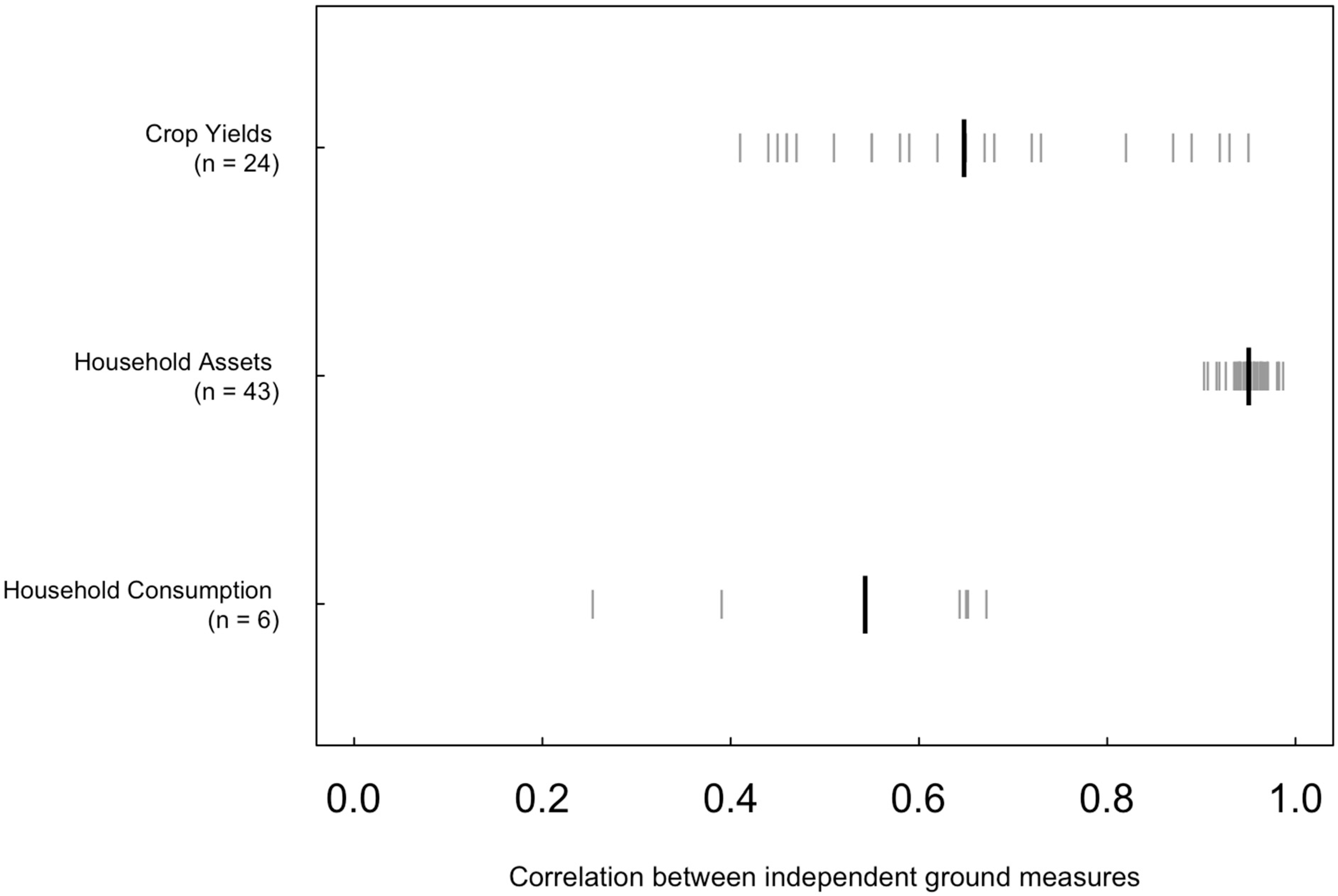
3.1. Correlations between Ground Measures

Figure 1 presents a quantitative summary of one straightforward measure of noise in typical ground data—the correlation between two independent ground measures of the same outcome. For the case of crop yields, we identified all studies with at least two crop-cuts per field (Table S1) and report the correlation across all sampled fields of the first and second crop-cut (or the mean correlation if there are more than two crop-cuts). For household wealth and consumption, we used public datasets (see Section 2) and for each survey enumeration area (or “cluster”, roughly equivalent to village in rural areas) we split surveyed households into two random subsets of equal size, computed the average values for each subset, and then reported the correlation across clusters between the two subcluster averages.
Overall, both crop yields and household consumption exhibit considerable noise, with correlations commonly below 0.7. This indicates that in a typical setting, less than half of the variation in a measured outcome can be explained by an independent measure of that exact same outcome, at the same location (i.e., field or village), using the exact same instrument (i.e., crop-cut or household survey). Notably, measures of household assets appear more robust, perhaps reflecting the larger number of households typically surveyed in a cluster for DHS (mean of 25) compared to LSMS surveys (mean of 10), the fact that asset ownership is easier to recall and verify, or some combination of these and other factors. Given the higher correlations for asset measures, we focus below on correcting performance measures for yields and household consumption and leave aside the issue of correcting performance measures for household assets.

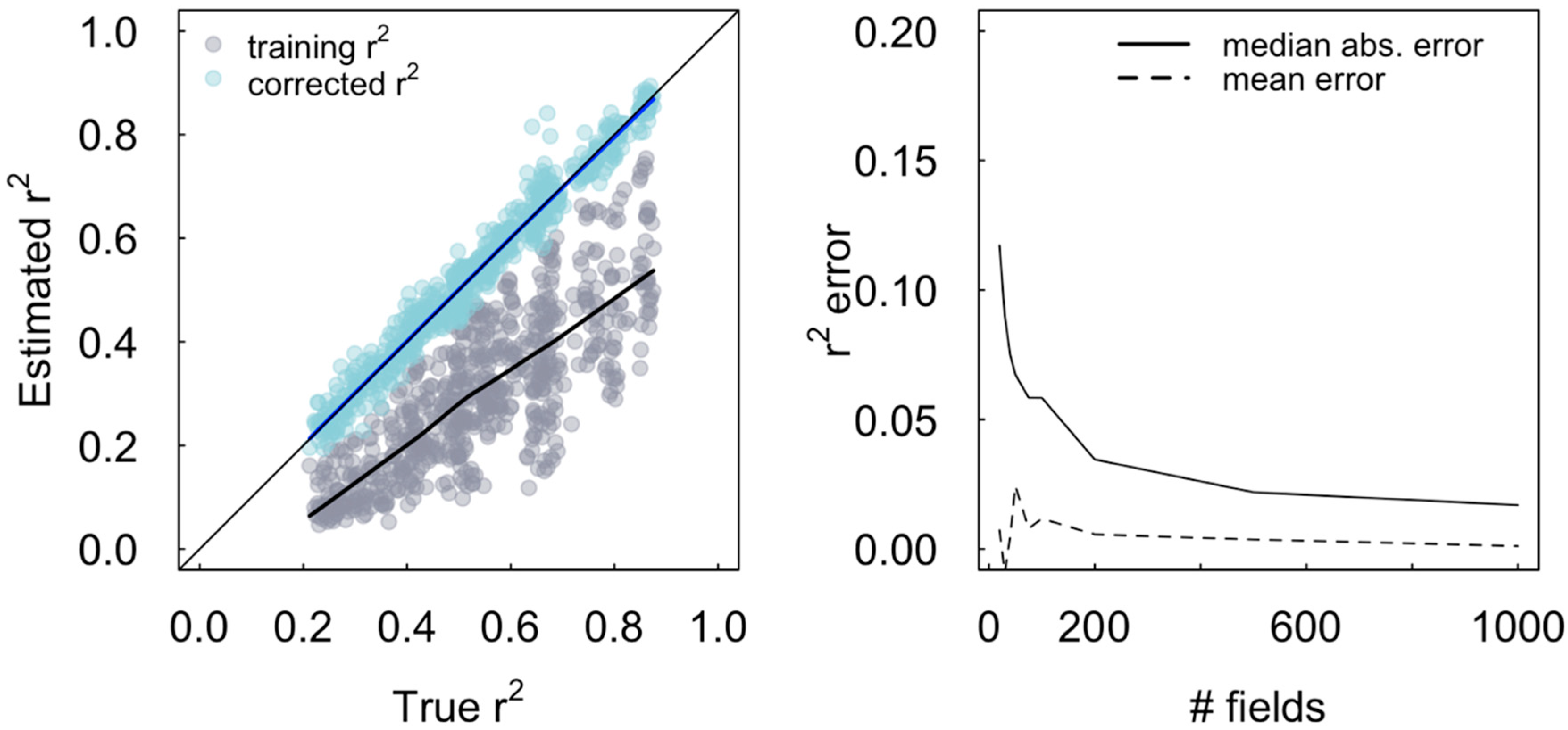
3.2. Simulations Illustrate the Value of Two Ground Measures

We begin by testing the validity of Equation (14) for different sample sizes using a series of simple simulations. In particular, the derivation of Equation (14) rested on the assumption that the covariance between two noisy measures of yield is exactly σy2, which is true in the limit since the covariance between independent realizations of noise will be zero. However, for finite samples of noise (σS, σG1, σG2), these covariances will generally be slightly larger or smaller than zero, leading to a question of how accurate Equation (14) will be under typical conditions.
To address this question, we turn to a set of simple simulations as described in the Methods. Figure 2a compares the true r2(S,Y) with both r2(S,G1) (e.g., the training r2 for a satellite model trained on a noisy ground measure) and the estimated r 2 ^ ( S , Y ) based on Equation (14). This initial plot pertains to a large number of locations (N = 1000) to illustrate two key points. First, the training r2 is always less than the true r2, and can be well below 50% of the true value. Second, Equation (14) results in an unbiased estimate of the true r2 across a range of parameter combinations, with most points falling very close to the 1:1 line. Equation (14) remains valid even if one assumes that satellite estimates are subject to Berkson rather than the classical measurement error, with values that are smoother (i.e., have less variance) than the true values (Figure S1).
We then implement the simulations using a smaller number of locations (N ranging from 20 to 1000) to evaluate how performance of Equation (14) could vary as the number of fields with which to calculate the relevant terms declines. The results reveal that while the mean error across multiple simulations remains close to zero, the median absolute error is higher for smaller sample sizes (Figure 2b). The median absolute error reaches as high as 0.10 for a sample of 20 locations, but is below 0.05 for sample sizes above ~100. These simulations indicate that Equation (14) will still perform well on average when applied to datasets with fewer than 100 fields, but that the variance of the performance will increase as the number of fields decrease.

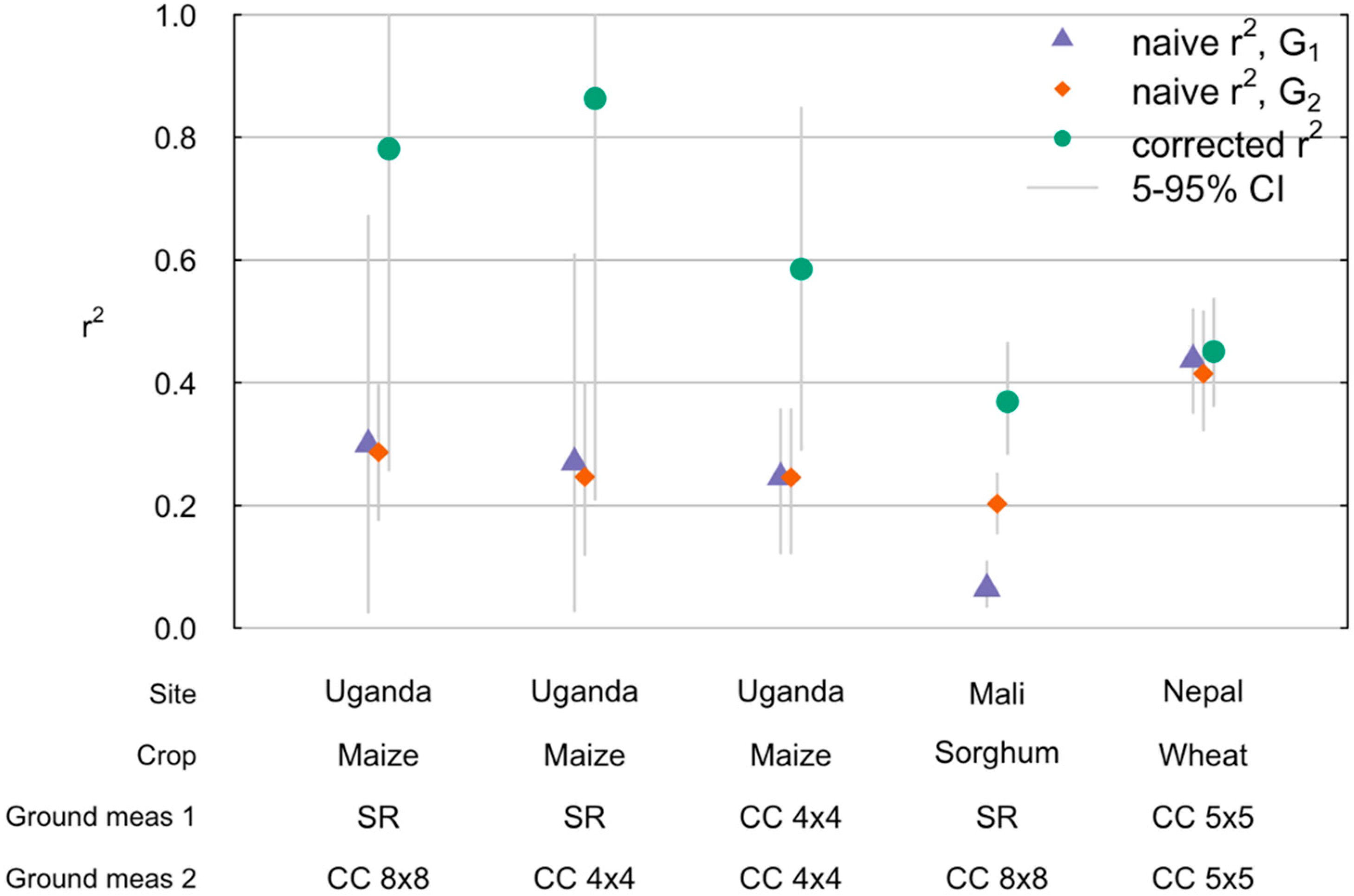
3.3. Correcting for Ground Noise Significantly Improves Performance Measures for Crop Yields

To illustrate the application of Equation (14) for crop yields, we reconsider some prior published remote sensing studies where more than one ground measure was available (Figure 3). Specifically, we compare the agreement of satellite-yield estimates with each individual ground measure, and then apply Equation (14) to estimate a “corrected” r2. We also compute a 5–95% confidence interval for each measure of r2 by resampling the data with replacement 100 times, calculating the r2 values for each sample, and taking the 5th and 95th highest values out of the 100 bootstrap samples.
In a study of pure stand maize fields in Uganda for 2016 [11], three different ground-based measures were collected: self-report yields, 8 × 8 m crop-cuts, and 4 × 4 m crop-cuts. When combining self-report yields with either of the crop-cuts, the corrected r2 using Equation (14) is above 0.8, more than twice the uncorrected values albeit with wide confidence intervals. When using two 4 × 4 m crop-cuts as the two ground measures, the corrected r2 is lower at 0.52. In this study, we also obtained a full plot harvest for a subset of fields [11], which if treated as the truth provides a direct estimate of r2(S,Y) of 0.56. Thus, the corrected r2 for the 4 × 4 m crop-cuts was very similar to the direct estimate of the true value. The corrected r2 values when using self-report were also consistent with the true value but exhibited wide error bars owing to the smaller number of fields with both self-report and crop-cut data.
In a study of 557 sorghum fields in Mali [21], satellite-based yields exhibited an r2 of 0.07 and 0.20 with self-report and crop-cut yields, respectively. In contrast, the corrected r2 was considerably higher at 0.37, because of the low observed correlation between self-report and crop-cuts (r = 0.32). In a study of 147 wheat fields in Nepal, two separate 5 × 5 m crop-cuts were obtained in each field, with a high correlation of 0.93 between them despite the fact that they were reportedly independent samples. This could reflect the fact that these wheat fields were irrigated, which tends to increase the homogeneity of yield outcomes. As a result of the higher correlation between crop-cuts, the corrected r2 of 0.45 was only slightly higher than the training r2 for the individual crop-cuts (of 0.41 and 0.43).

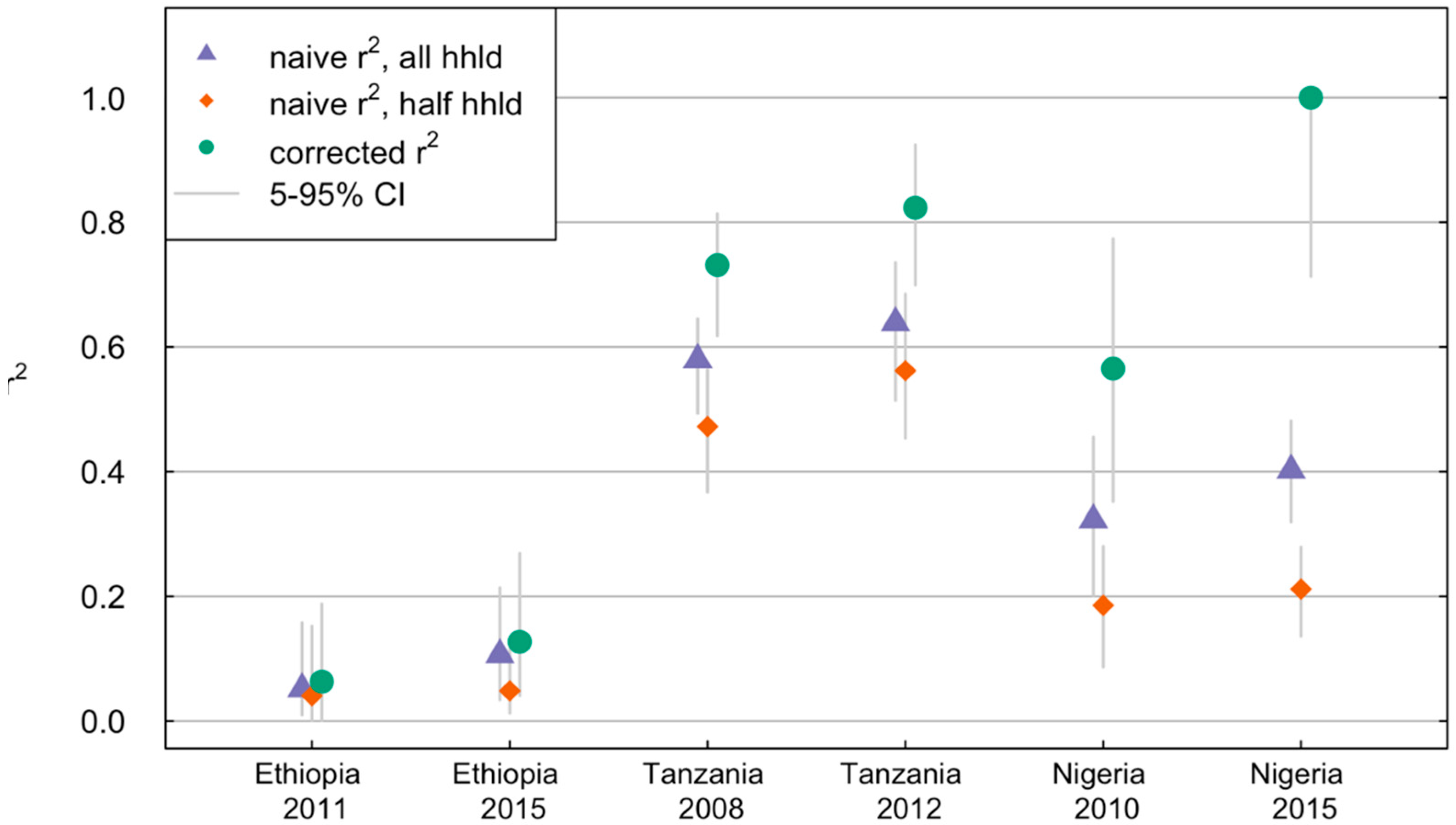
3.4. Correcting for Ground Noise Significantly Improves Performance Measures for Household Consumptions

As with crop yields, household consumption expenditures are difficult to measure with traditional ground-based instruments, resulting in low correlations between two independent measures (Figure 1). For six country–year combinations, we trained a single model to estimate consumption based on the distribution of satellite nighttime lights (NL) (see Section 2). Although more complicated models using high-resolution daytime imagery are possible [1,23], a model using NL distribution has been shown to perform nearly as well as the best models, and serves the purpose here of providing a credible satellite-based estimate. The model was trained using 60% of data from each country-year, with the remaining 40% used to test the model.
Performance (r2) on the held-out test data was estimated using the naïve comparison, where all households in a cluster were used to estimate average consumption, as well as using Equation (14) with G1 defined as the average of a random half of the households and G2 as the average of the other half (Figure 4). For comparison, we also show how the naïve r2 changes if using only half of the households (G1). Consistent with the notion that sampling more households helps to reduce noise in the ground-based estimate, the naïve r2 was higher in all six cases when using the average of all households rather than half of the households. However, the corrected r2, which explicitly accounts for noise in the ground-based measures, was higher still, especially in Tanzania and Nigeria. Corrected r2 in Ethiopia remained low, mainly because nightlights appear to explain very little variation in ground-measured household consumption (the numerator in Equation (14) is close to zero).
On average, the corrected r2 was 0.2 points higher than the naïve r2 for consumption expenditures across the six cases, with a median difference of 0.16. Interestingly, this difference is similar in magnitude to the difference in many countries between satellite performance for predicting assets vs. consumption [1,20]. Thus, although on the surface it appears that assets are “easier” than consumption to predict from satellite, it may be that much of the difference, in fact, arises from the fact that consumption is harder to measure than assets on the ground.

3.5. Correcting Satellite Performance Measures in the Absence of Two Ground-Based Estimates

One main argument of this paper is that researchers should strive to obtain two independent ground-based measures of an outcome of interest in order to properly assess the performance of satellite-based measures. In the case of household surveys, this implies splitting households within a location into two groups rather than combining them into one. In the case of crop yields, this implies collecting two small crop-cuts rather than one large one. Yet we recognize that for various reasons this may not be feasible in some situations and, therefore, offer a few points for proceeding with only a single ground measure. First and foremost, the r2 between satellite and ground measures should be reported with an emphasis on the downward bias that results from noise in the ground measure.
Second, one can still use Equation (14) with an estimate of how well a second measure of the same type would correlate with the first (as in the example of the 4 × 4 m crop-cuts in Uganda). The correlations in Figure 1 can provide some indication of plausible values for these correlations.
Third, in situations where errors in ground-based measures are due partly to spatial heterogeneity, as in the case of yield crop-cuts, one can use a map of satellite-based estimates themselves to assess the likely correlation between two independent ground-based measures. This approach assumes that (i) imperfect correlation between two crop-cuts arises primarily from in-field yield heterogeneity rather than measurement error for the crop-cut area itself, and (ii) satellite-based yields can adequately characterize in-field spatial heterogeneity. For the latter condition, it is likely important that the resolution of the satellite data be close to the size of the crop-cut area.
To test this approach, we return to the Uganda and Mali examples above, where we have one 8 m × 8 m crop-cut as well as yield maps based on the 10 m × 10 m Sentinel-2 imagery. We randomly sampled two pixels from within each field and calculated the correlation between the two samples across all fields. The corrected r2 was then calculated as:
r 2 ( S , Y ) =   r ( S , G 1 ) 2   r ( S 1 , S 2 )  
where S is the satellite-based yield estimate for the entire field, G1 is the crop-cut yield, and S1 and S2 are the satellite estimates for the two sampled pixels. This calculation is repeated 100 times, each time taking a new sample of fields and of pixels within the fields, to estimate a confidence interval on the corrected r2.
The median correlation between two independently sampled pixels in each field was 0.38 for maize in Uganda and 0.70 for sorghum in Mali. The corrected r2 that results from combining these correlations with the single crop-cut (Equation (17)) agreed well with the corrected r2 from using the combination of self-report and crop-cut (Equation (14) (Figure 5). Thus, at least for these two examples, it appears that using satellite measures of in-field heterogeneity can be a useful substitute for two independent ground measures of yield.

4. Discussion

The notion that having two noisy ground-based measures allows one to recover the true correlation of S with an outcome is perhaps counter-intuitive. Indeed, to our knowledge, studies that have taken multiple ground measures typically combine these into an average before comparing with satellite measures. However, the notion that three noisy but independent measures of a quantity can be used to infer the true values is well established in other fields, such as the triple collocation methods used for remote sensing of wind speed or soil moisture [24,25]. Whereas those approaches are focused on estimating the true value at locations with three noisy observations, here we are concerned with the related problem of measuring the correlation of one easily scalable measurement (e.g., satellite measures) with the true unobserved values, by employing two additional independent measures at a small number of locations.
Several remaining issues deserve future attention. First, while our correction approach assumes the availability of two independent ground measures, many situations are likely to arise when the ground measures are not perfectly independent. Self-report yields, for instance, are prone to many sources of non-classical measurement error including mistaken beliefs [26] that could be correlated with errors in the crop-cut yield, or could themselves be affected by farmer awareness of crop-cut values. Similarly, errors in measuring household expenditures could be correlated across households in the same cluster, for instance if households in a certain region have common incentives to over- or under-report. We note that, to the extent these measurement errors are positively correlated, as is plausibly the case for both yields and consumption, our corrected performance estimates from Equation (14) will understate true performance. Future work should probe the likely bias from Equation (14) in the presence of non-independent ground measures, as well as potential remedies in these situations.
Second, while our focus here is on characterizing the overall performance of satellite measures, future work could attempt to estimate (and correct for) the error for individual observations. This could be achieved, for example, by using triple colocation methods for locations where two ground measures are available, or by identifying covariates that are predictive of deviations between satellite and ground measures.
Third, there are many-development-relevant variables that we did not consider in the current study, such as population density or the existence of informal settlements [4]. More work is needed to establish approaches to quantify the degree of noise in ground data for these variables, characterize the magnitude of this noise, and re-evaluate the performance of satellite measures in light of these errors.

5. Conclusions

With increased availability of satellite remote sensing data and growing interest in lowering the cost and improving the accuracy of economic statistics, we anticipate continued growth in studies aimed at characterizing outcomes, such as crop yields and household wealth using satellite data. Based on the results presented here, we offer a few key points for future work.
First, be wary of using unadjusted correlations between satellite and ground measures to evaluate performance, given that these can substantially underestimate true performance. Second, whenever possible, try to obtain at least two independent ground-based measures of an outcome. For outcomes measured in household surveys, this can be readily achieved by splitting households into two independent groups within each location (i.e., cluster). For outcomes measured by other means, such as in the case of crop-cuts for yield estimation, we recommend prioritizing two measures for each field, even if they are fairly small. For example, two 2 m × 2 m crop-cuts would be more valuable than one 4 m × 4 m crop-cut.
Third, if only one ground-measure is available, adjustments can still be made, either by using a range of values for noise from the literature or using satellite-based measures of correlations between pixels sampled from the same location (i.e., within fields as in Figure 4). If only one ground-measure is available, we also advise relying less on head-to-head comparisons between satellite and ground-based measures, and more on collecting measures of factors that are likely to influence the outcome, such as fertilizer use or soil quality in the case of crop yields. One can then perform regressions that examine the outcome response to these factors, with attention to whether regression coefficients have similar or better precision when using satellite-based rather than ground-based measures [10,11,17]. In these situations, the ability to uncover response coefficients is a more useful indicator of the accuracy of satellite-based outcomes than a direct comparison to a noisy ground-based measure [4].

Supplementary Materials

The following are available online at https://www.mdpi.com/article/10.3390/rs13163160/s1, Figure S1: Simulations with Berkson error, Figure S2: Crop-cut correlations by crop, Table S1: Crop-cut correlations by study, Table S2: Self-report correlations with crop-cut, Table S3: Uganda correlations for adjacent and random crop-cut locations.

Author Contributions

Conceptualization, D.B.L. and M.B.; methodology, D.B.L.; formal analysis, D.B.L., S.D.T.; resources, D.B.L., M.B., T.K.; writing—original draft preparation, D.B.L.; writing—review and editing, M.B., T.K. All authors have read and agreed to the published version of the manuscript.

Funding

This research was funded by USAID Bureau for Food Security, the Global Innovation Fund, and NASA Harvest Consortium, NASA Applied Sciences Grant No. 80NSSC17K0625, sub-award 54308-Z6059203 to D.B.L.

Institutional Review Board Statement

Not applicable.

Informed Consent Statement

Not applicable.

Data Availability Statement

All data used in this study are available from the authors upon request.

Acknowledgments

We thank Anne Driscoll for assistance with the DHS and LSMS datasets, Marie-Julie Lambert, Pierre Defourny, and Jake Campolo for providing data from their yield studies, Peter Craufurd and the TAMASA program for making their data publicly available, and Chris Barrett for helpful comments on an earlier draft of the manuscript.

Conflicts of Interest

The authors declare no conflict of interest. The funders had no role in the design of the study; in the collection, analyses, or interpretation of data; in the writing of the manuscript, or in the decision to publish the results.

References

  1. Jean, N.; Burke, M.; Xie, M.; Davis, W.M.; Lobell, D.B.; Ermon, S. Combining satellite imagery and machine learning to predict poverty. Science 2016, 353, 790–794. [Google Scholar] [CrossRef] [Green Version]
  2. Blumenstock, J.; Cadamuro, G.; On, R. Supplementary Materials for Predicting poverty and wealth from mobile phone metadata. Science 2015, 350, 1073–1076. [Google Scholar] [CrossRef] [PubMed] [Green Version]
  3. Sheehan, E.; Meng, C.; Jean, N.; Tan, M.; Burke, M.; Ermon, S.; Uzkent, B.; Lobell, D. Predicting economic development using geolocated wikipedia articles. In Proceedings of the 25th ACM SIGKDD International Conference on Knowledge Discovery and Data Mining, Anchorage, AK, USA, 4–8 August 2019. [Google Scholar]
  4. Burke, M.; Driscoll, A.; Lobell, D.B.; Ermon, S. Using satellite imagery to understand and promote sustainable development. Science 2021, 371, eabe8628. [Google Scholar] [CrossRef]
  5. Watmough, G.R.; Marcinko, C.L.J.; Sullivan, C.; Tschirhart, K.; Mutuo, P.K.; Palm, C.A.; Svenning, J.C. Socioecologically informed use of remote sensing data to predict rural household poverty. Proc. Natl. Acad. Sci. USA 2019, 116, 1213–1218. [Google Scholar] [CrossRef] [PubMed] [Green Version]
  6. Mirza, M.U.; Xu, C.; van Bavel, B.; van Nes, E.H.; Scheffer, M. Global inequality remotely sensed. Proc. Natl. Acad. Sci. USA 2021, 118, e1919913118. [Google Scholar] [CrossRef]
  7. Clevers, J.G.P.W. A simplified approach for yield prediction of sugar beet based on optical remote sensing data. Remote Sens. Environ. 1997, 61, 221–228. [Google Scholar] [CrossRef]
  8. Lobell, D.B.; Asner, G.P.; Ortiz-Monasterio, J.I.; Benning, T.L. Remote sensing of regional crop production in the Yaqui Valley, Mexico: Estimates and uncertainties. Agric. Ecosyst. Environ. 2003, 94, 205–220. [Google Scholar] [CrossRef] [Green Version]
  9. Lambert, M.J.; Traoré, P.C.S.; Blaes, X.; Baret, P.; Defourny, P. Estimating smallholder crops production at village level from Sentinel-2 time series in Mali’s cotton belt. Remote Sens. Environ. 2018, 216, 647–657. [Google Scholar] [CrossRef]
  10. Burke, M.; Lobell, D.B. Satellite-based assessment of yield variation and its determinants in smallholder African systems. Proc. Natl. Acad. Sci. USA 2017, 114, 2189–2194. [Google Scholar] [CrossRef] [Green Version]
  11. Lobell, D.B.; Azzari, G.; Burke, M.; Gourlay, S.; Jin, Z.; Kilic, T.; Murray, S. Eyes in the Sky, Boots on the Ground: Assessing Satellite- and Ground-Based Approaches to Crop Yield Measurement and Analysis. Am. J. Agric. Econ. 2019, 1–18. [Google Scholar] [CrossRef]
  12. Jain, M.; Singh, B.; Srivastava, A.; McDonald, A.; Lobell, D.B. Mapping Smallholder Wheat Yields and Sowing Dates Using Micro-Satellite Data. Remote Sens. 2016, 8, 860. [Google Scholar] [CrossRef] [Green Version]
  13. Johnson, D.M. An assessment of pre- and within-season remotely sensed variables for forecasting corn and soybean yields in the United States. Remote Sens. Environ. 2014, 141, 116–128. [Google Scholar] [CrossRef]
  14. World Bank Group. Capacity Needs Assessment for Improving Agricultural Statistics in Kenya; World Bank Publications: Washington, DC, USA, 2016. [Google Scholar]
  15. World Bank Group. Capacity Needs Assessment for Improving Agricultural Statistics in Uganda; World Bank Publications: Washington, DC, USA, 2016. [Google Scholar]
  16. Carletto, C.; Jolliffe, D.; Banerjee, R. From Tragedy to Renaissance: Improving Agricultural Data for Better Policies. J. Dev. Stud. 2015, 51, 133–148. [Google Scholar] [CrossRef]
  17. Gourlay, S.; Kilic, T.; Lobell, D.B. A new spin on an old debate: Errors in farmer-reported production and their implications for inverse scale—Productivity relationship in Uganda. J. Dev. Econ. 2019, 141, 102376. [Google Scholar] [CrossRef]
  18. FAO. Handbook on Crop Statistics: Improving Methods for Measuring Crop Area, Production and Yield; FAO: Rome, Italy, 2018. [Google Scholar]
  19. Fermont, A.; Benson, T. Estimating Yield of Food Crops Grown by Smallholder Farmers: A Review in the Uganda Context; International Food Policy Research Institute: Washington, DC, USA, 2011. [Google Scholar]
  20. Yeh, C.; Perez, A.; Driscoll, A.; Azzari, G.; Tang, Z.; Lobell, D.; Ermon, S.; Burke, M. Using publicly available satellite imagery and deep learning to understand economic well-being in Africa. Nat. Commun. 2020, 11, 2583. [Google Scholar] [CrossRef]
  21. Lobell, D.B.; Di Tommaso, S.; You, C.; Djima, I.Y.; Burke, M.; Kilic, T. Sight for sorghums: Comparisons of satellite-and ground-based sorghum yield estimates in Mali. Remote Sens. 2020, 12, 100. [Google Scholar] [CrossRef] [Green Version]
  22. Campolo, J.; Güereña, D.; Maharjan, S.; Lobell, D.B. Evaluation of soil-dependent crop yield outcomes in Nepal using ground and satellite-based approaches. Field Crops Res. 2021, 260, 107987. [Google Scholar] [CrossRef]
  23. Ayush, K.; Uzkent, B.; Tanmay, K.; Burke, M.; Lobell, D.; Ermon, S. Efficient Poverty Mapping from High Resolution Remote Sensing Images. Proc. AAAI Conf. Artif. Intell. 2021, 35, 12–20. [Google Scholar]
  24. Scipal, K.; Holmes, T.; De Jeu, R.; Naeimi, V.; Wagner, W. A possible solution for the problem of estimating the error structure of global soil moisture data sets. Geophys. Res. Lett. 2008, 35, 2–5. [Google Scholar] [CrossRef] [Green Version]
  25. Stoffelen, A. Toward the true near-surface wind speed: Error modeling and calibration using triple collocation. J. Geophys. Res. Oceans 1998, 103, 7755–7766. [Google Scholar] [CrossRef]
  26. Abay, K.A.; Bevis, L.E.M.; Barrett, C.B. Measurement Error Mechanisms Matter: Agricultural Intensification with Farmer Misperceptions and Misreporting. Am. J. Agric. Econ. 2020, 103, 498–522. [Google Scholar] [CrossRef]
Figure 1. Noise in ground-based measures can lead to low correlations between independent measures in the same location. Gray lines show estimates of the correlation between two independent measures, with one line for each separate dataset, and black line shows the mean value across datasets. Individual studies and sources for crop yields are presented in Table S1. For household assets, we used data from DHS for 23 countries, with 1–4 years per country. For consumption estimates, we used data from LSMS for three countries, with two years per country. The mean number of fields for crop-cut studies was 145. The mean number of clusters for asset surveys was 462, with an average of 25 households per cluster. The mean number of clusters for consumption surveys was 161, with a mean of 10 households per cluster.
Remotesensing 13 03160 g001
Figure 2. Simulated performance of Equation (14) to correct the measure of satellite performance for noise in ground data. (left) Training r2 (gray points) and corrected r2 (blue points, using Equation (14)) for a linear regression model that predicts ground-measured yields with satellite-measured yields for 1000 fields, plotted against the “true” r2 between satellite-measured and true yields. True yields and the noisy ground- and satellite-based measures of yields were simulated from Equations (4)–(8), (11) and (12), with each point representing a single set of simulation parameters, and simulations then repeated for different combinations of parameter values to span a wide range of r2. Lines show a locally-weighted polynomial (LOWESS) fit to the points. Parameters ranged from 1 to 3 t/ha for sY, and 0.5 to 3 t/ha for σ ϵ S , σ ϵ G 1 , and σ ϵ G 2 . The value of m was fixed at 5 t/ha, since varying this value does not affect the resulting r2. Overall, training r2 underestimates the true r2, whereas Equation (14) results in an unbiased estimate of the true r2. (right) The difference between the true and corrected r2 (from Equation (14)) plotted against the number of fields simulated. The mean difference (i.e., bias) remains small when a small number of fields are simulated, but the median absolute error rises sharply when fewer than 100 fields are measured.
Remotesensing 13 03160 g002
Figure 3. Naïve r2 understates true performance for satellite crop yield estimation. Comparison of r2 between satellite-based yields and two different ground-based measures of yields, as well as a corrected r2 using Equation (14). The confidence intervals (gray bars) were calculated by resampling the fields and recalculating the different r2 values. The bottom panel indicates the location, crop, and type of ground measures used. Uganda data are from [11], Mali data from [21], and Nepal data from [22].
Remotesensing 13 03160 g003
Figure 4. Naïve r2 understates true performance for satellite household consumption estimation. Comparison of r2 between satellite-based consumption expenditure estimates and household surveys for six country-year combinations. Naïve r2 show estimates when directly comparing satellite estimates to the average value for all or half of households in each cluster, while corrected r2 uses Equation (14) with G1 and G2 each based on half of the households in each cluster. The confidence intervals (gray bars) were calculated by resampling the clusters and recalculating the different r2 values.
Remotesensing 13 03160 g004
Figure 5. Satellite measures of in-field heterogeneity can substitute for a second crop-cut. Comparison of naive r2 for a regression of satellite-based yields on crop-cut yields (G1), the corrected r2 using self-report yields and Equation (14) as in Figure 3 (method 1), and corrected r2 using satellite-based estimates of the correlation between two crop-cuts and Equation (15) (method 2). The confidence intervals (gray bars) were calculated by resampling the fields and recalculating the different r2 values.
Remotesensing 13 03160 g005
Publisher’s Note: MDPI stays neutral with regard to jurisdictional claims in published maps and institutional affiliations.

