Communication

The Impact of Seasonality and Response Period on Qualifying the Relationship between Ecosystem Productivity and Climatic Factors over the Eurasian Steppe

1
College of Earth and Planetary Sciences, University of Chinese Academy of Sciences, Beijing 100049, China
2
Key Laboratory of Digital Earth Science, Aerospace Information Research Institute, Chinese Academy of Sciences, Beijing 100094, China
3
National Academy of Economic Strategy, Chinese Academy of Social Sciences, Beijing 102488, China
*
Author to whom correspondence should be addressed.
Remote Sens. 2021, 13(16), 3159; https://doi.org/10.3390/rs13163159
Submission received: 29 June 2021 / Revised: 2 August 2021 / Accepted: 5 August 2021 / Published: 10 August 2021
(This article belongs to the Special Issue Remote Sensing of Grassland Ecosystem)

Abstract

:
As climate change intensifies, surface vegetation productivity and carbon exchange between terrestrial ecosystems and the atmosphere are significantly affected by the variation of climatic factors. Due to the sensitivity of grasslands to these climatic factors, it is crucial to understand the response of vegetation greenness, or carbon exchange within grasslands, to environment factor dynamics. In this study, we used solar-induced chlorophyll fluorescence (SIF), precipitation (P), vapor pressure deficit (VPD), evaporative stress (ES), and root zone soil moisture (RSM) derived from remote sensing, reanalysis, and assimilation datasets to explore the response of vegetation greenness within Eurasian Steppe to climatic factors. Our results indicated deseasonlization based on the Seasonal-Trend decomposition using Loess (STL) method, which was an effective means to remove the seasonality disturbances that affect the qualification of the relationship between SIF and the four climatic factors. The response of SIF had a time lag effect on these climatic factors, and the longer the response period, the greater the impact on the correlation of SIF with P, VPD, ES, and RSM. We also found, among the four factors, that the response of SIF to ES was the timeliest. The findings of this study emphasized the impact of the seasonality and time lag effect on the dynamic response between variables, and provided references to the attribution and monitoring of vegetation greenness and ecosystem productivity.

Graphical Abstract

1. Introduction

Irregular changes of environmental factors caused by climate change have significant impacts on the change of surface vegetation growth, resulting in erratic carbon exchange between terrestrial ecosystem and the atmosphere [1]. Grasslands are a potentially important sink for carbon in the terrestrial biosphere because of the high levels of carbon accrual and sequestration below ground in the soil, and up to 90% of grassland biomass is below ground. The levels of soil carbon are higher in grasslands than in forests, agroecosystems, or other ecosystems [2,3]. Carbon cycling within grasslands is sensitive to climatic factors [4] and vulnerable to climate change [5,6,7]. As climate change intensifies, it is crucial to understand the response of vegetation greenness or carbon exchange within grassland to environment factors’ dynamics.
Normally, the carbon exchange between terrestrial ecosystem and the atmosphere is quantified by gross primary productivity (GPP) and ecosystem respiration (RE) [8,9]. The solar-induced chlorophyll fluorescence (SIF), which is an optical signal emitted in the spectral range 650–850 nm from the chlorophyll a molecule in vegetation [10], demonstrates a tight relationship with photosynthesis at the ecosystem scale through ground-based and airborne hyperspectral measurements [11,12,13]. The global SIF observations from satellites have become available in recent years, which has led to tremendous developments in monitoring terrestrial photosynthesis and ecosystem productivity (i.e., GPP) at various spatial and temporal scales, which caused SIF to be increasingly used as a proxy for GPP on large scales [14,15,16]. Additionally, SIF was utilized to characterize vegetation greenness [17], determine the vegetation growing season [18], estimate evapotranspiration [19], and the like. Climatic factors, such as precipitation, temperature, solar radiation, transpiration, evaporation, soil moisture, etc., influence land-atmosphere carbon exchange through their impact on vegetation growth and greenness. Precipitation is the primary connection in the water cycle that provides for the delivery of atmospheric water to the Earth, and it controls ecosystem dynamics and drives biological processes [20,21]. The appropriate temperature and solar radiation, which are usually used as input variables in the calculation of some indices, are the elements that ensure the normal growth of vegetation [22]. The vapor pressure deficit (VPD) is calculated from the near-surface temperature and relative humidity, which can characterize the water stress in the air [23,24]. The soil moisture provides available water to vegetation roots and represents the water stress from the soil [25,26]. Evapotranspiration is the sum of transpiration from vegetation and the evaporation from the soil and land surface, and the important connection in the water cycle between the atmosphere and the land [27,28,29].
A clear understanding of the responses of vegetation productivity or ecosystem carbon uptake to the above climatic factors is helpful to extreme events monitoring, mechanism model establishment, etc. Previous studies evaluated the vegetation response to changes in air temperature [30,31], precipitation [32,33,34], and solar radiation [35,36], but fewer climatic variables were involved. However, since the response periods of vegetation to different climatic factors are diverse, it is also necessary to concurrently consider the relationships between grasslands and multiple climatic factors [37].
Here, we used SIF, precipitation (P), VPD, evaporative stress (ES), and root-zone soil moisture (RSM) derived from remote sensing, reanalysis, and assimilation datasets, to explore the responses of vegetation growth and productivity to climatic factors over the Eurasian Steppe. Before this, the deseasonlization method based on the Seasonal and Trend decomposition using Loess (STL) and Pearson’s correlation coefficient were utilized to probe the impact of seasonality/periodicity and the lag phases on qualifying the relationship between SIF and the four climatic factors. These two methods were also used to remove the disturbance of periodicity and to determine the response period between SIF and climatic factors.

2. Materials and Methods

2.1. Study Area

Grasslands, which are among the most prominent biogeographic regions on the Earth for human welfare and livestock, cover a wide range of vegetation types and geographic locations [7,38,39,40]. Eurasia contains nearly double the amount of total grassland ecoregions of the other continents [41]. The grasslands (27–125°E, 27–57°N, Figure 1) in Eurasia were thus selected as the study area, and it is the largest continuously continental grasslands in the world. The region has a complex topography such as lowlands, large plains, and high mountains, and is dominated by a temperate continental climate with hot summers and cold winters [42]. In addition, the precipitation in this area varies greatly from the northwest to the southeast. In recent decades, the grasslands are experiencing degradation and desertification caused by agriculture activities and disasters, which led to carbon loss from the grasslands. For degraded soils within the grassland, recovery is slow, taking 50 or more years [2]. These all result in damage to rangelands that are essential for animal husbandry development, regional ecological security, and sustainability [43].

2.2. Data

2.2.1. Land Cover

The Moderate Resolution Imaging Spectroradiometer (MODIS) Land Cover Climate Modeling Grid Product (MCD12C1) was created using the supervised classification of MODIS reflectance data, and provides maps of the International Geosphere-Biosphere Program (IGBP), the University of Maryland (UMD), and the leaf area index (LAI) schemes at a 0.05° spatial resolution per year [44]. In this study, we followed the IGBP classification principle to extract the grasslands in the study area.

2.2.2. Solar-Induced Chlorophyll Fluorescence (SIF)

Solar-induced fluorescence (SIF) is mechanistically linked to photosynthesis and is shown to have a near-linear relationship with ecosystem GPP at the ecosystem scale [45,46]. In this study, the global ‘OCO-2’ SIF (GOSIF) dataset was used as the indicator of ecosystem productivity (i.e., GPP). The GOSIF was developed by Li and Xiao [13] using discrete OCO-2 SIF soundings, remote sensing data from the moderate resolution imaging spectroradiometer (MODIS), and meteorological reanalysis data through Cubist regression tree model. The GOSIF has a 0.05° spatial resolution and an 8-day and monthly temporal resolution. This product was available from March 2000 to December 2020.

2.2.3. Precipitation (P)

The Global Precipitation Measurement (GPM) precipitation dataset, which is organized as an international project led by the National Aeronautics and Space Administration (NASA) and the Japanese Space Agency (JAXA), is an international network of satellites that provide next-generation global observations of rain and snow [47]. Building upon the success of the Tropical Rainfall Measuring Mission (TRMM), the GPM concept centers on the deployment of a “Core” satellite carrying an advanced radar/radiometer system to measure precipitation from space and serve as a reference standard to unify precipitation measurements from a constellation of research and operational satellites. The Integrated Multi-satellitE Retrievals for GPM (IMERG) Level3 V06 monthly “Final” precipitation product with a 0.1° spatial resolution was used as a precipitation variable for climatic factors.

2.2.4. Air Temperature (T) and Relative Humidity (RH)

In this study, we used air temperature and relative humidity derived from the fifth generation of the European Centre for Medium-Range Weather Forecasts (ECMWF) atmospheric reanalysis (ERA 5) to calculate the VPD. The air temperature within the ERA 5 is the temperature of the air at 2 m above the surface of land, sea, or in-land waters, and calculated by interpolating between the lowest model level and the Earth’s surface, taking account of the atmospheric conditions. The relative humidity is the ratio of the partial pressure of water vapor to the equilibrium vapor pressure of water at the same temperature near the surface. Both have a 0.25° spatial resolution and monthly temporal resolution [48].

2.2.5. Evaporative Stress (ES) and Root Zone Soil Moisture (RSM)

The Global Land Evaporation Amsterdam Model (GLEAM) is designed to estimate the land surface evaporation and root zone soil moisture from remote sensing observations and reanalysis data [49,50]. Specifically, the Priestley-Taylor equation is used to calculate potential evaporation within the GLEAM based on the near-surface temperature and net radiation, while the root zone soil moisture is obtained from a multilayer water balance driven by precipitation observations and updated with the microwave soil moisture estimates [50]. The actual evaporation is estimated by constraining potential evaporation with a multiplicative evaporative stress factor based on the root zone soil moisture and vegetation optical depth estimates. The GLEAM version 3.5a provides the global daily and monthly potential and actual evaporation, evaporative stress conditions, and the root zone soil moisture from 1980 to 2020 at a spatial resolution of 0.25° (http://www.gleam.eu, accessed on 20 May 2021). In this study, the GLEAM v3.5a root zone soil moisture and evaporative stress were used.
The time period of SIF, P, T, RH, ES, and RSM we used in this study were from January 2001 to December 2020, and the 2001–2019 MCD12C1 land cover product was used. With regard to the spatial resolution, through the resample method which was ‘nearest’ in ArcGIS (https://desktop.arcgis.com/zh-cn/arcmap/10.6/map/main/mapping-and-visualization-in-arcgis-for-desktop.htm, accessed on 1 June 2021) version 10.6, we resampled the GPM precipitation (0.1°) and the GOSIF (0.05°) to 0.25°, that is, the same as the ERA5 and GLEAM datasets, which also meant the resolution of the pixel used in the next study and analysis was 0.25° × 0.25°.

2.3. Methods

2.3.1. Seasonal-Trend Decomposition Using Loess (STL)

The STL can decompose a time-series into additive components (trend, seasonality/periodicity, and the remainder) of variation by the application of loess smoothing models [51,52]. Further information on the method and parameters can be found in the original paper describing the STL method [53]. In this study, we used the STL to extract the seasonality of the time series of the variables mentioned (SIF, P, VPD, RSM, and ES) across each pixel over the study area. Then, we obtained the deseasonalized time series of this variables through the use of the observed time series minus the seasonal time series. The goal was achieved by Python 3.7 (https://www.python.org/, accessed on 4 June 2021) and the statsmodels library (https://www.statsmodels.org/dev/generated/statsmodels.tsa.seasonal.STL.html, accessed on 4 June 2021).

2.3.2. Pearson’ s Correlation Coefficient (r)

The Pearson’s correlation coefficient is a method that is based on using the covariance matrix of the data to evaluate the strength of the linear relationship between two variables. Normally, the Pearson’s correlation coefficient between two variables is [53]:
r ( x , y ) = i = 1 n [ ( x i x ¯ ) × ( y i y ¯ ) ] i = 1 n ( x i x ¯ ) 2 × i = 1 n ( y i y ¯ ) 2
where x ¯ and y ¯ denote the means of the two variables, and n is the sample number (length of the time series).
In this study, the Pearson’s correlation coefficient was utilized to determine the response periods between SIF and climatic factors (P, VPD, ES, and RSM). For example, on each pixel over the grasslands, we first calculated the r between deseasonalized time series of SIF and P (r (SIFds, Pds)). The deseasonalized P time series was moved one or more positions (one or more months) forward, then they were used to recalculate the correlation with deseasonalized SIF time series (r (SIFds, Pds1), r (SIFds, Pds2), …). We compared these r to ascertain the response period of SIF to P, more specifically, if the r (SIFds, Pds2) was the maximum, the response period was between two and three months (i.e., the lag phase of SIF to P was two months).
In this study, all maps and figures were created by Python 3.7, and the cartopy (https://pypi.org/project/Cartopy/, accessed on 4 June 2021) and matplotlib (https://matplotlib.org/, accessed on 4 June 2021) libraries. The hardware and storage employed were the Inter(R) Xeon(R) Gold 5218 CPU @ 2.30 GHz 2.29 GHz and 192 GB Random Access Memory with 2 TB Read-Only Memory. The operating system was 64-bit Windows 10.

3. Results

3.1. The Impact of Seasonality on the Relationship of SIF to P, VPD, ES and RSM Dynamics

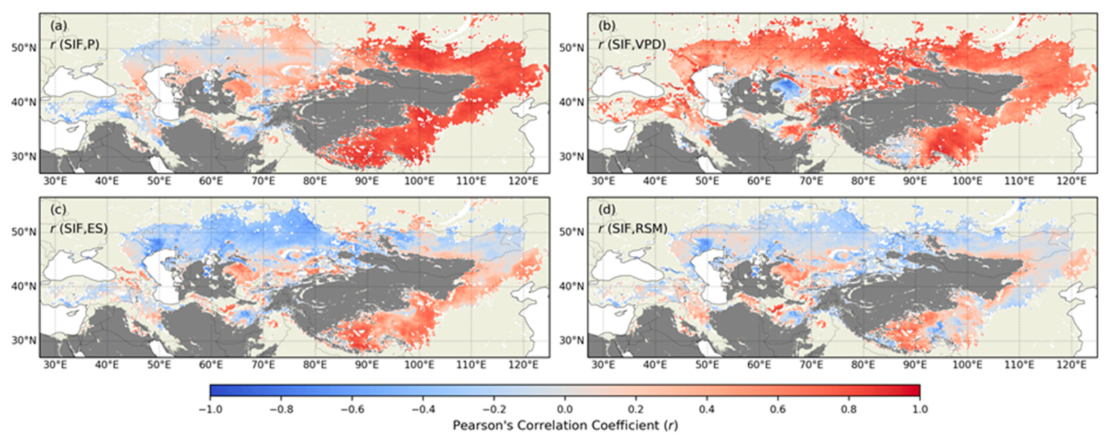
Firstly, we calculated the spatial r maps of SIF with P, VPD, ES, and RSM, without any time series adjustment (Figure 2). According to the mechanism relationship between SIF and the four climatic factors, P, ES, and RSM have positive correlations with SIF, and VPD has a negative correlation with SIF. However, in Figure 2, the spatial r of original SIF with the original P (r (SIF, P)), VPD (r (SIF, VPD)), ES (r (SIF, ES)), and RSM (r (SIF, RSM)) did not follow the mechanism. More specifically, in the spatial maps of r (SIF, P) (Figure 2a), r (SIF, ES) (Figure 2c), and r (SIF, RSM) (Figure 2d), there were large areas of negative r values, while in the spatial maps of r (SIF, VPD) (Figure 2b), the r values were almost positive.
We conducted further research and found that the seasonality/periodicity of the time series led to the anomalous phenomenon. We compared the original and deseasonlized time series between SIF and RSM at 50°N and 70°E (Figure 3) and found the original time series of SIF and RSM (Figure 3a) had clear seasonality and the dynamic response between SIF and RSM were inconspicuous, while Figure 3b showed a legible response between the deseasonlized time series of SIF (SIFds) and RSM (RSMds) dynamics. These indicated that seasonality affected the qualification of the relationship between SIF and the four factors, and even led to incorrect results. Therefore, for qualifying the relationship between SIF and the four climatic factors, the impacts of seasonality need to be removed. Simultaneously, the deseasonalization based on the STL method was a useful means of removing the disturbance generated by periodicity.
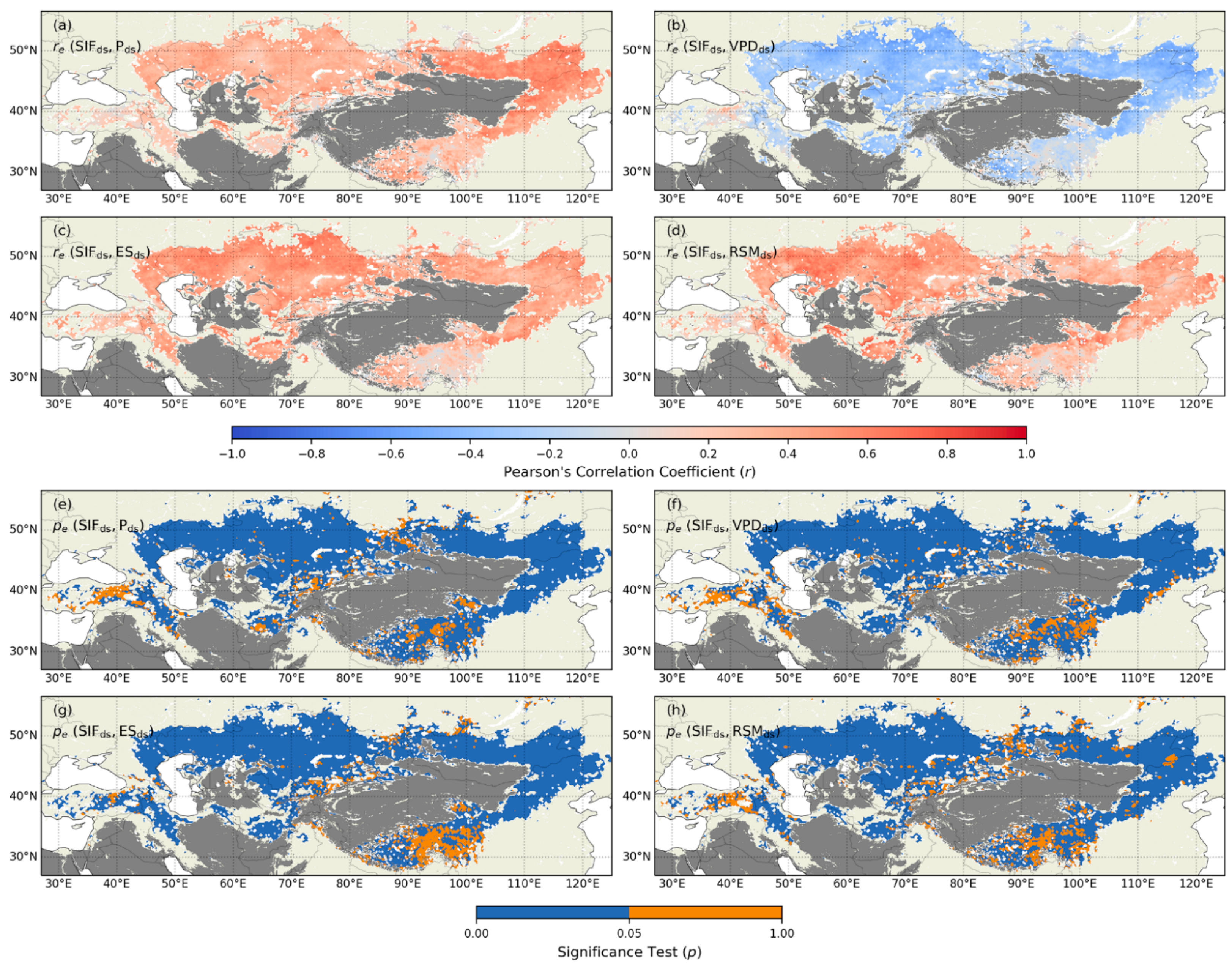
After deseasonalizing the time series of SIF, P, VPD, ES, and RSM (SIFds, Pds, VPDds, ESds, and RSMds) based on the STL method, we recalculated the spatial correlation between SIFds and the four factors (Figure 4). Overall, the spatial r maps followed the mechanism mentioned above, and ES correlated with SIF best. However, there were still unreasonable r values between SIF and the four factors. For example, between the 90°E and 100°E, in the northern and southern regions of the grasslands, the r (SIFds, VPDds) were greater than zero, which they should had been negative correlations between SIF and VPD according to the response mechanism between them. In addition, the corresponding spatial maps of p showed a large area which did not pass the significance test (p > 0.05). The area with an insignificant r between P and SIF (Figure 4e) was the greatest, while that between ES and SIF (Figure 4g) was the lowest. The p value maps of SIF with VPD (Figure 4f) and RSM (Figure 4h) had analogous spatial distribution.

3.2. The Influence of Response Period on r of SIF with P, VPD, ES and RSM

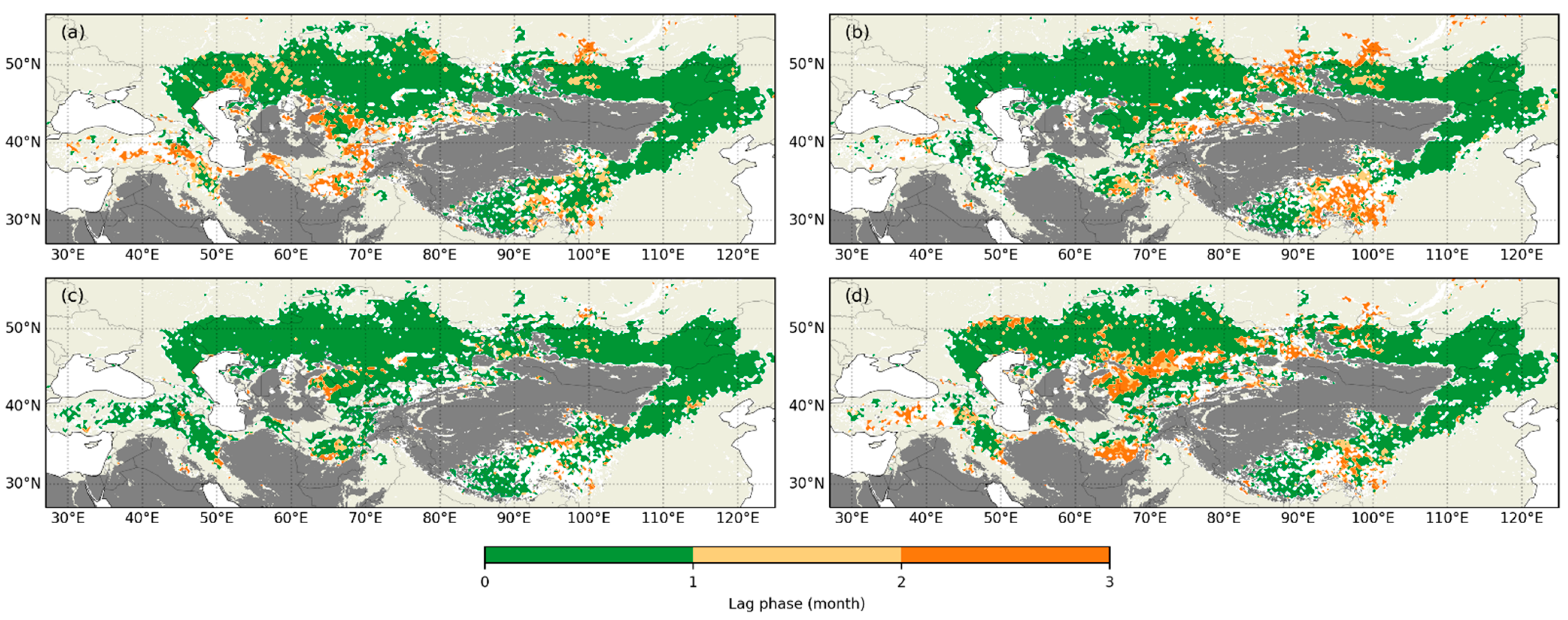
Certainly, the delayed response of SIF to the four climatic factors means there are time lag effects between them. By using the methods mentioned in Section 2.3, we determined the lag phases of SIF to the four factors (Figure 5, masked by the significant extremum r of SIF to the four climatic factors). SIF had a time lag effect on the four factors over the grasslands and the lag phases were mainly within one month. Combing Figure 4 and Figure 5, the spatial r of SIF with P, VPD, ES, and RSM were consistent with the spatial lag phase maps of SIF to the four factors. Specifically, poor (p > 0.05) or opposite correlations between SIF and these factors were mainly located in areas with lag phases greater than one month. Collectively, the r values were affected by the response periods and the longer the period, the greater the impact. In addition, in Figure 5, the area with response periods of SIF to ES of more than one month were the lowest among the four factors, which meant the response of SIF to ES was timely.
We integrated the maximum r of SIF with P, ES, and RSM and the minimum r of SIF with VPD, and the corresponding spatial p maps were also integrated (Figure 6). Compared with Figure 4, the spatial r maps were more reasonable, and the qualification of the relationship between SIF and climatic factor was improved (by comparing the colors). The overall spatial r of SIF with P, VPD, ES, and RSM in Figure 6 showed improvement, especially in the areas with poor or even inverse correlations. Additionally, the areas with p > 0.05 were noticeably decreased. Since the extremum r values were obtained by adjusting the time series, this indicated that the delayed response of SIF to the four climatic factors, or the time lag between them, impacted the assessment and qualification of the relationship among variables.
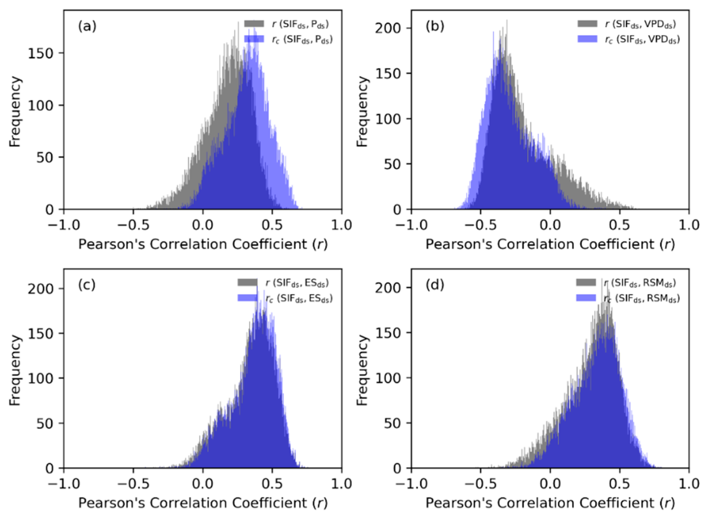
In addition, we conducted comparative statistical analyses (shown in Figure 4 and Figure 6), and the results (Figure 7) showed that all of the r of SIF with the four factors were improved. The improvement of the r of SIF with P and ES were the largest and the smallest, respectively, which suggested the response period affected the correlation of SIF to P the most and the correlation to ES was the least affected among the four factors. The response period, or time lag effect, also has different degrees of influence on evaluating and qualifying the relationship between vegetation growth or ecosystem productivity and the climatic factors. All of these indicated that the correlation of SIF with P, VPD, ES, and RSM were impacted by the time lag effect. In addition, though we corrected the spatial r of SIF with the four variables, there were poor r values in some areas; the reason for this may be that vegetation greenness and productivity are affected by multiple variables, and a single variable cannot fully explain the vegetation greenness and productivity dynamics.

4. Discussion

4.1. Methods of Deseasonlization

Section 3.1 showed that the seasonality/periodicity seriously impacted the qualification of the relationship between SIF and the climatic factors. We eliminated the seasonality disturbance through the STL method. In fact, differencing and classical decomposition methods were also widely used to deseasonalize the seasonality of the time series [54], and these methods can be implemented by computer languages such as Python and R. However, both of them have weaknesses. Differencing refers to using the next cycle minus the time series of this cycle, which will reduce a cycle of the observations. For the data of this study, a cycle is a year, and the difference method will thus reduce the length of the original time series by one year. For classical decomposition methods, there are two forms of classical decomposition: an additive decomposition and a multiplicative decomposition [55]. They assume that the seasonal component repeats from year to year, which means they are unable to capture these seasonal changes over time. Classical decomposition methods are also unable to handle outliers properly. The STL method does not have these problems, and it can be robust to outliers. Although the STL method does not handle trading day or calendar variation automatically and only provides facilitation for additive decompositions, it does not affect the extraction of the seasonality of SIF and the four factors [52]. We believe that the STL method can play a greater role in the field of natural sciences.

4.2. The Determination of Lag Phase

In this study, by comparing the maximum or minimum value of Pearson’s correlation coefficient (r), we determined the lag phase, which is inspired by the studies of Peng et al. [56] and Xie et al. [57]. Our results showed a delayed response or time lag effect which impacted the correlation between SIF and the climatic factors. However, there were some uncertainties in this method. More specifically, Figure 6 could be considered as correcting the r of SIF with the four factors through adjusting the time series of SIF and the four factors to a reasonable response period. Compared with Figure 4, the spatial maps of p were noticeably improved in Figure 6. In fact, we adjusted the time series within 6 months, but in some areas the r of SIF with the climatic factors were insignificant at any adjustment. For this situation, we cannot determine the lag phases between variables, or even analyze the response between them. In addition, the correlation coefficient is a measure of the overall relationship between two variables. However, in the study period, some events, such as droughts and floods, made the relationship between SIF and the climatic factors abnormal or even deviant. This also affected the assessment and qualification of the mechanism of the relationship between variables. For determining a more accurate lag phase or response period, we believe that it is more effective to study the response between the variables from the perspective of events and utilize higher temporal and spatial resolution data.

4.3. The Impact of Time Lag Effect on Ecosystem and Climatic Change

The time lag effect of major climatic driving forces on phenology should be paid more attention to improve the prediction and evaluation of vegetation response [56,58,59]. An increasing number of studies have found that the responses of vegetation to climate has a certain time lag [60,61,62,63,64,65]. Braswell et al., researched the interannual lag of vegetation’s response to temperature among various ecosystems [30]. Wang et al., found the spatial pattern of the normalized difference vegetation index (NDVI) is strongly correlated with the longer time intervals of precipitation than with recent precipitation [66]. Anderson et al., investigated the time-lag effects for different climatic factors (i.e., radiation, rainfall, and aerosol optical depth) in the Amazon and found that the time lag of the vegetation responses to the climatic factors differed in the rainforest [58]. The vegetation responses to soil moisture lagged by approximately one month over the Australian mainland [64]. These studies recognize the importance of the time lag effects of vegetation responses to climate. The four climatic factors, P, VPD, ES, and RSM, were related to the vegetation water stress. Our findings showed the SIF mainly lagged behind these factors by one month, and in small areas the lag phases were within two and three months. This was similar to the results of Zhao et al. [67], which found the NDVI lagged behind standardized precipitation and the evapotranspiration index (SPEI, a drought index which can characterize water stress) within 2–3 month over grassland vegetation in the Chinese Loess Plateau (102°54′–114°33′E, 33°43′–41°16′N). The results of Zuo et al., displayed that the NDVI has a one-month lag effect on precipitation over the grassland of the Yarlung Zangbo River Basin (82°00′–97°07′E, 28°00′–31°16′N), which is the same as our results in this region [68]. Collectively, vegetation growth may not be primarily driven by present climatic conditions, but earlier climatic conditions may also have impact on vegetation growth. Therefore, the time lag effects should be considered when exploring the mechanisms of climate-vegetation interactive effects.
Actually, most studies that focused on large-scale climate-vegetation interactions adopted the simultaneous climatic and vegetation indicators, and the time lag effects were minimally considered, which would increase the uncertainty of the results. For example, the composite drought index involved in hydrological, meteorological, and ecological variables only combined these variables by methods such as linear combination, regression, and weight combination, and did not consider the time lag effects between them. When using drought indices to monitor and assess vegetation drought, most studies did not consider the response mechanism or time lag effect, leading to uncertainties in the results [26]. Additionally, for the estimation of terrestrial variables in ecological and hydrological process [69], for instance evapotranspiration, the estimation may involve more variables than were used in building a composite drought index. The time lag effects among various variables also need to be carefully considered in related models, which may improve the accuracy of the estimate. In fact, as climate change intensifies, climatic system become anomalous. We need more accurate results, whether in the monitoring and prediction of natural disasters or the estimation of surface variables. Taking the response mechanisms or time lag effect into account may be a potential direction to achieve this end.

4.4. Limitations and Prospects

There were limitations in this study. The length of the response period may not be accurate enough, since the temporal resolution of the datasets we used were monthly. With regard to the spatial r of SIF with the four variables, there were insignificant or poor r values in some areas after adjusting the time series of variables. The potential reason for this was that a single climatic variable change cannot fully explain the vegetation greenness or productivity dynamics. We did not comprehensively utilize P, VPD, ES, and RSM to explore and analyze the response of SIF to a combined indictor or index. In future studies, we will combine multiple climatic factors to generate a composite indictor to explore its relationship with vegetation growth, ecosystem productivity, or carbon exchange. We will also utilize higher temporal and spatial resolution datasets to determine the response period of the ecosystem to climatic factors. We will also extend the study area to larger regions with diverse vegetation types in order to analyze the dynamic response between different vegetation types and climatic factors.

5. Conclusions

In this study, we utilized SIF, P, VPD, ES, and RSM to explore the response of vegetation greenness or productivity to the climatic factor dynamics over the Eurasian Steppe. Our findings showed the seasonality of the variables’ time series created disturbance in qualifying the relationship between SIF and the climatic factors, and the deseasonalization based on the STL method was an effective means to remove the disturbance of periodicity. The response of SIF to P, VPD, ES, and RSM all had time lag effects, and the response period had an impact on the correlation of SIF with the four climatic factors. Among P, VPD, ES, and RSM, P was the most affected by the response period, while ES was the least impacted by the response period. This study provides a reference for researchers to attribute and monitor the dynamics of ecosystem productivity and carbon exchange.

Author Contributions

Conceptualization, Q.L. (Qi Liu), X.M. and H.Z.; Funding acquisition, J.Z. and F.Y.; Methodology, Q.L. (Qi Liu); Project administration, J.Z. and F.Y.; Resources, Q.L. (Qi Liu); Software, Q.L. (Quan Liu); Supervision, J.Z. and F.Y.; Validation, X.M. and J.Z.; Visualization, Q.L. (Quan Liu); Writing—original draft, Q.L. (Qi Liu); Writing—review & editing, J.Z. All authors have read and agreed to the published version of the manuscript.

Funding

This research was funded by the Chinse Academy of Sciences Strategic Priority Research Program (Grant: No. XDA19030402), the National Natural Science Foundation of China (Grant: Nos. 42071425, 41871253), and the Taishan Scholar Project of Shandong Province (Grant: No. TSXZ201712).

Institutional Review Board Statement

Not applicable.

Informed Consent Statement

Not applicable.

Data Availability Statement

Not applicable.

Acknowledgments

This study was supported by the CAS Strategic Priority Research Program (No. XDA19030402), the National Natural Science Foundation of China (Nos. 42071425, 41871253), and the Taishan Scholar Project of Shandong Province (No. TSXZ201712). We also thank editors and reviewers for providing comments and suggestion to improve the manuscript.

Conflicts of Interest

The authors declare no conflict of interest.

References

  1. Zheng, K.; Tan, L.; Sun, Y.; Wu, Y.; Duan, Z.; Xu, Y.; Gao, C. Impacts of climate change and anthropogenic activities on vegetation change: Evidence from typical areas in China. Ecol. Indic. 2021, 126, 107648. [Google Scholar] [CrossRef]
  2. Faber-Langendoen, D. Tropical, Temperate, and Mediterranean Grasslands of the World. In Encyclopedia of the World’s Biomes; Michael, I.G., Dominick, A.D., Eds.; Elsevier: Amsterdam, The Netherlands, 2020; pp. 424–433. [Google Scholar]
  3. Wilson, S. Grasses and grassland ecology. Ann. Bot. 2009, 104. [Google Scholar] [CrossRef] [Green Version]
  4. Flanagan, L.B.; Wever, L.A.; Carlson, P.J. Seasonal and interannual variation in carbon dioxide exchange and carbon balance in a northern temperate grassland. Glob. Chang. Biol. 2002, 8, 599–615. [Google Scholar] [CrossRef]
  5. Baldocchi, D.; Chu, H.; Reichstein, M. Inter-annual variability of net and gross ecosystem carbon fluxes: A review. Agric. For. Meteorol. 2018, 249, 520–533. [Google Scholar] [CrossRef] [Green Version]
  6. Thornton, P.K.; van de Steeg, J.; Notenbaert, A.; Herrero, M. The impacts of climate change on livestock and livestock systems in developing countries: A review of what we know and what we need to know. Agric. Syst. 2009, 101, 113–127. [Google Scholar] [CrossRef]
  7. Wang, R.; Gamon, J.A.; Emmerton, C.A.; Springer, K.R.; Yu, R.; Hmimina, G. Detecting intra- and inter-annual variability in gross primary productivity of a North American grassland using MODIS MAIAC data. Agric. For. Meteorol. 2020, 281, 107859. [Google Scholar] [CrossRef]
  8. Liu, H.; Jia, J.; Lin, Z.; Wang, Z.; Gong, H. Relationship between net primary production and climate change in different vegetation zones based on EEMD detrending—A case study of Northwest China. Ecol. Indic. 2021, 122, 107276. [Google Scholar] [CrossRef]
  9. Piao, S.; Fang, J.; Zhou, L.; Zhu, B.; Tan, K.; Tao, S. Changes in vegetation net primary productivity from 1982 to 1999 in China. Glob. Biogeochem. Cycles 2005, 19, GB2027. [Google Scholar] [CrossRef] [Green Version]
  10. Lichtenthaler, H.K.; Buschmann, C.; Rinderle, U.; Schmuck, G. Application of chlorophyll fluorescence in ecophysiology. Radiat. Environ. Biophys. 1986, 25, 297–308. [Google Scholar] [CrossRef]
  11. Yang, X.; Tang, J.; Mustard, J.F.; Lee, J.E.; Rossini, M.; Joiner, J.; Munger, J.W.; Kornfeld, A.; Richardson, A.D. Solar-induced chlorophyll fluorescence that correlates with canopy photosynthesis on diurnal and seasonal scales in a temperate deciduous forest. Geophys. Res. Lett. 2015, 42, 2977–2987. [Google Scholar] [CrossRef]
  12. Damm, A.; Guanter, L.; Paul-Limoges, E.; van der Tol, C.; Hueni, A.; Buchmann, N.; Eugster, W.; Ammann, C.; Schaepman, M.E. Far-red sun-induced chlorophyll fluorescence shows ecosystem-specific relationships to gross primary production: An assessment based on observational and modeling approaches. Remote Sens. Environ. 2015, 166, 91–105. [Google Scholar] [CrossRef]
  13. Li, X.; Xiao, J. A global, 0.05-degree product of solar-induced chlorophyll fluorescence derived from OCO-2, MODIS, and reanalysis data. Remote Sens. 2019, 11, 517. [Google Scholar] [CrossRef] [Green Version]
  14. Xiao, J.; Chevallier, F.; Gomez, C.; Guanter, L.; Hicke, J.A.; Huete, A.R.; Ichii, K.; Ni, W.; Pang, Y.; Rahman, A.F.; et al. Remote sensing of the terrestrial carbon cycle: A review of advances over 50 years. Remote Sens. Environ. 2019, 233, 111383. [Google Scholar] [CrossRef]
  15. Ryu, Y.; Berry, J.A.; Baldocchi, D.D. What is global photosynthesis? History, uncertainties and opportunities. Remote Sens. Environ. 2019, 223, 95–114. [Google Scholar] [CrossRef]
  16. Dechant, B.; Ryu, Y.; Badgley, G.; Zeng, Y.; Berry, J.A.; Zhang, Y.; Goulas, Y.; Li, Z.; Zhang, Q.; Kang, M.; et al. Canopy structure explains the relationship between photosynthesis and sun-induced chlorophyll fluorescence in crops. Remote Sens. Environ. 2020, 241, 111733. [Google Scholar] [CrossRef] [Green Version]
  17. Liu, L.; Gudmundsson, L.; Hauser, M.; Qin, D.; Li, S.; Seneviratne, S.I. Soil moisture dominates dryness stress on ecosystem production globally. Nat. Commun. 2020, 11, 4892. [Google Scholar] [CrossRef]
  18. Jeong, S.J.; Schimel, D.; Frankenberg, C.; Drewry, D.T.; Fisher, J.B.; Verma, M.; Berry, J.A.; Lee, J.E.; Joiner, J. Application of satellite solar-induced chlorophyll fluorescence to understanding large-scale variations in vegetation phenology and function over northern high latitude forests. Remote Sens. Environ. 2017, 190, 178–187. [Google Scholar] [CrossRef]
  19. Shan, N.; Zhang, Y.; Chen, J.M.; Ju, W.; Migliavacca, M.; Peñuelas, J.; Yang, X.; Zhang, Z.; Nelson, J.A.; Goulas, Y. A model for estimating transpiration from remotely sensed solar-induced chlorophyll fluorescence. Remote Sens. Environ. 2021, 252, 112134. [Google Scholar] [CrossRef]
  20. Nemani, R.R.; Keeling, C.D.; Hashimoto, H.; Jolly, W.M.; Piper, S.C.; Tucker, C.J.; Myneni, R.B.; Running, S.W. Climate-driven increases in global terrestrial net primary production from 1982 to 1999. Science 2003, 300, 1560–1563. [Google Scholar] [CrossRef] [Green Version]
  21. Notaro, M.; Liu, Z.; Gallimore, R.G.; Williams, J.W.; Gutzler, D.S.; Collins, S. Complex seasonal cycle of ecohydrology in the Southwest United States. J. Geophys. Res. Biogeosci. 2010, 115, G04034. [Google Scholar] [CrossRef]
  22. Li, D.; Wu, S.; Liang, Z.; Li, S. The impacts of urbanization and climate change on urban vegetation dynamics in China. Urban For. Urban Green. 2020, 54, 126764. [Google Scholar] [CrossRef]
  23. Rawson, H.M.; Begg, J.E.; Woodward, R.G. The effect of atmospheric humidity on photosynthesis, transpiration and water use efficiency of leaves of several plant species. Planta 1977, 134, 5–10. [Google Scholar] [CrossRef]
  24. Yuan, W.; Zheng, Y.; Piao, S.; Ciais, P.; Lombardozzi, D.; Wang, Y.; Ryu, Y.; Chen, G.; Dong, W.; Hu, Z.; et al. Increased atmospheric vapor pressure deficit reduces global vegetation growth. Sci. Adv. 2019, 5, eaax1396. [Google Scholar] [CrossRef] [Green Version]
  25. Liu, Q.; Zhang, S.; Zhang, H.; Bai, Y.; Zhang, J. Monitoring drought using composite drought indices based on remote sensing. Sci. Total Environ. 2020, 711, 134585. [Google Scholar] [CrossRef]
  26. Liu, Q.; Zhang, J.; Zhang, H.; Yao, F.; Bai, Y.; Zhang, S.; Meng, X.; Liu, Q. Evaluating the performance of eight drought indices for capturing soil moisture dynamics in various vegetation regions over China. Sci. Total Environ. 2021, 789, 147803. [Google Scholar] [CrossRef] [PubMed]
  27. Bai, Y.; Zhang, S.; Bhattarai, N.; Mallick, K.; Liu, Q.; Tang, L.; Im, J. On the use of machine learning based ensemble approaches to improve evapotranspiration estimates from croplands across a wide environmental gradient. Agric. For. Meteorol. 2021, 298–299, 108308. [Google Scholar] [CrossRef]
  28. Bai, Y.; Zhang, J.; Zhang, S.; Yao, F.; Magliulo, V. A remote sensing-based two-leaf canopy conductance model: Global optimization and applications in modeling gross primary productivity and evapotranspiration of crops. Remote Sens. Environ. 2018, 215, 411–437. [Google Scholar] [CrossRef]
  29. Bai, Y.; Zhang, S.; Zhang, J.; Wang, J.; Yang, S.; Magliulo, V.; Vitale, L.; Zhao, Y. Using remote sensing information to enhance the understanding of the coupling of terrestrial ecosystem evapotranspiration and photosynthesis on a global scale. Int. J. Appl. Earth Obs. Geoinf. 2021, 100, 102329. [Google Scholar] [CrossRef]
  30. Braswell, B.H.; Schimel, D.S.; Linder, E.; Moore, B. The response of global terrestrial ecosystems to interannual temperature variability. Science 1997, 278, 870–873. [Google Scholar] [CrossRef]
  31. Root, T.L.; Price, J.T.; Hall, K.R.; Schneider, S.H.; Rosenzweig, C.; Pounds, J.A. Fingerprints of global warming on wild animals and plants. Nature 2003, 421, 57–60. [Google Scholar] [CrossRef]
  32. Nemani, R.; White, M.; Thornton, P.; Nishida, K.; Reddy, S.; Jenkins, J.; Running, S. Recent trends in hydrologic balance have enhanced the terrestrial carbon sink in the United States. Geophys. Res. Lett. 2002, 29, 106-1–106-4. [Google Scholar] [CrossRef] [Green Version]
  33. Fay, P.A.; Kaufman, D.M.; Nippert, J.B.; Carlisle, J.D.; Harper, C.W. Changes in grassland ecosystem function due to extreme rainfall events: Implications for responses to climate change. Glob. Chang. Biol. 2008, 14, 1600–1608. [Google Scholar] [CrossRef]
  34. Chen, Z.; Wang, W.; Fu, J. Vegetation response to precipitation anomalies under different climatic and biogeographical conditions in China. Sci. Rep. 2020, 10, 830. [Google Scholar] [CrossRef] [PubMed] [Green Version]
  35. Kong, D.; Zhang, Q.; Singh, V.P.; Shi, P. Seasonal vegetation response to climate change in the Northern Hemisphere (1982–2013). Glob. Planet. Chang. 2017, 148, 1–8. [Google Scholar] [CrossRef] [Green Version]
  36. Nanzad, L.; Zhang, J.; Batdelger, G.; Pangali Sharma, T.P.; Koju, U.A.; Wang, J.; Nabil, M. Analyzing NPP Response of Different Rangeland Types to Climatic Parameters over Mongolia. Agronomy 2021, 11, 647. [Google Scholar] [CrossRef]
  37. Zhong, R.; Wang, P.; Mao, G.; Chen, A.; Liu, J. Spatiotemporal variation of enhanced vegetation index in the Amazon Basin and its response to climate change. Phys. Chem. Earth 2021, 123, 103024. [Google Scholar] [CrossRef]
  38. Singh, J.S.; Lauenroth, W.K.; Milchunas, D.G. Geography of grassland ecosystems. Prog. Phys. Geogr. 1983, 7, 46–80. [Google Scholar] [CrossRef]
  39. Sala, O.E.; Lauenroth, W.K.; McNaughton, S.J.; Rusch, G.; XinShi, Z.; Mooney, H.A.; Cushman, J.H.; Medina, E.; Schulze, E.D. Biodiversity and ecosystem functioning in grasslands. In Functional Roles of Biodiversity: A Global Perspective; John Wiley & Sons Ltd.: Hoboken, NJ, USA, 1996. [Google Scholar]
  40. Wu, Z.; Zhang, J.; Deng, F.; Zhang, S.; Zhang, D.; Xun, L.; Javed, T.; Liu, G.; Liu, D.; Ji, M. Fusion of gf and modis data for regional-scale grassland community classification with evi2 time-series and phenological features. Remote Sens. 2021, 13, 835. [Google Scholar] [CrossRef]
  41. Dixon, A.P.; Faber-Langendoen, D.; Josse, C.; Morrison, J.; Loucks, C.J. Distribution mapping of world grassland types. J. Biogeogr. 2014, 41, 2003–2019. [Google Scholar] [CrossRef]
  42. Lioubimtseva, E.; Cole, R.; Adams, J.M.; Kapustin, G. Impacts of climate and land-cover changes in arid lands of Central Asia. J. Arid Environ. 2005, 62, 285–308. [Google Scholar] [CrossRef]
  43. Chen, T.; Tang, G.; Yuan, Y.; Guo, H.; Xu, Z.; Jiang, G.; Chen, X. Unraveling the relative impacts of climate change and human activities on grassland productivity in Central Asia over last three decades. Sci. Total Environ. 2020, 743, 140649. [Google Scholar] [CrossRef]
  44. Sulla-menashe, D.; Friedl, M.A. User Guide to Collection 6 MODIS Land Cover (MCD12Q1 and MCD12C1) Product. 2018. Available online: https://lpdaac.usgs.gov/documents/101/MCD12_User_Guide_V6.pdf?_ga=2.198563055.1574254467.1612099295-1804377720.1601472205 (accessed on 14 May 2021).
  45. Li, X.; Xiao, J.; He, B.; Altaf Arain, M.; Beringer, J.; Desai, A.R.; Emmel, C.; Hollinger, D.Y.; Krasnova, A.; Mammarella, I.; et al. Solar-induced chlorophyll fluorescence is strongly correlated with terrestrial photosynthesis for a wide variety of biomes: First global analysis based on OCO-2 and flux tower observations. Glob. Chang. Biol. 2018, 24, 3990–4008. [Google Scholar] [CrossRef] [PubMed]
  46. Frankenberg, C.; Fisher, J.B.; Worden, J.; Badgley, G.; Saatchi, S.S.; Lee, J.E.; Toon, G.C.; Butz, A.; Jung, M.; Kuze, A.; et al. New global observations of the terrestrial carbon cycle from GOSAT: Patterns of plant fluorescence with gross primary productivity. Geophys. Res. Lett. 2011, 38, L17706. [Google Scholar] [CrossRef] [Green Version]
  47. Tapiador, F.J.; Turk, F.J.; Petersen, W.; Hou, A.Y.; García-Ortega, E.; Machado, L.A.T.; Angelis, C.F.; Salio, P.; Kidd, C.; Huffman, G.J.; et al. Global precipitation measurement: Methods, datasets and applications. Atmos. Res. 2012, 104–105, 70–97. [Google Scholar] [CrossRef]
  48. Copernicus Climate Change Service: Essential Climate Variables for Assessment of Climate Variability from 1979 to Present, Product User Guide. Available online: https://datastore.copernicus-climate.eu/documents/ecv-for-climate-change/PUG-ecv-for-climate-change_v3.pdf (accessed on 14 May 2021).
  49. Miralles, D.G.; Holmes, T.R.H.; De Jeu, R.A.M.; Gash, J.H.; Meesters, A.G.C.A.; Dolman, A.J. Global land-surface evaporation estimated from satellite-based observations. Hydrol. Earth Syst. Sci. 2011, 15, 453–469. [Google Scholar] [CrossRef] [Green Version]
  50. Martens, B.; Miralles, D.G.; Lievens, H.; Van Der Schalie, R.; De Jeu, R.A.M.; Fernández-Prieto, D.; Beck, H.E.; Dorigo, W.A.; Verhoest, N.E.C. GLEAM v3: Satellite-based land evaporation and root-zone soil moisture. Geosci. Model Dev. 2017, 10, 1903–1925. [Google Scholar] [CrossRef] [Green Version]
  51. Chaloupka, M. Historical trends, seasonality and spatial synchrony in green sea turtle egg production. Biol. Conserv. 2001, 101, 263–279. [Google Scholar] [CrossRef]
  52. Cleveland, R.B.; Cleveland, W.S.; McRae, J.E.; Terpenning, I. STL: A Seasonal-Trend Decomposition Procedure Based on Loess (with Discussion). J. Off. Stat. 1990, 6, 3–73. [Google Scholar]
  53. Wuensch, K.L.; Evans, J.D. Straightforward Statistics for the Behavioral Sciences. J. Am. Stat. Assoc. 1996, 91, 1750. [Google Scholar] [CrossRef]
  54. Hyndman, R.J.; Athanasopoulos, G. Forecasting: Principles and Practice, 2nd ed.; OTexts: Melbourne, Australia, 2018. [Google Scholar]
  55. Kendall, M.G.; Stuart, A. The Advanced Theory of Statistics. Vol. 3. Biometrics 1969, 25, 435. [Google Scholar] [CrossRef]
  56. Peng, J.; Wu, C.; Zhang, X.; Wang, X.; Gonsamo, A. Satellite detection of cumulative and lagged effects of drought on autumn leaf senescence over the Northern Hemisphere. Glob. Chang. Biol. 2019, 25, 2174–2188. [Google Scholar] [CrossRef]
  57. Xie, X.; Li, A.; Tan, J.; Lei, G.; Jin, H.; Zhang, Z. Uncertainty analysis of multiple global GPP datasets in characterizing the lagged effect of drought on photosynthesis. Ecol. Indic. 2020, 113, 106224. [Google Scholar] [CrossRef]
  58. Anderson, L.O.; Malhi, Y.; Aragão, L.E.O.C.; Ladle, R.; Arai, E.; Barbier, N.; Phillips, O. Remote sensing detection of droughts in Amazonian forest canopies. New Phytol. 2010, 187, 733–750. [Google Scholar] [CrossRef] [PubMed]
  59. Wu, D.; Zhao, X.; Liang, S.; Zhou, T.; Huang, K.; Tang, B.; Zhao, W. Time-lag effects of global vegetation responses to climate change. Glob. Chang. Biol. 2015, 21, 3520–3531. [Google Scholar] [CrossRef]
  60. Davis, M.B. Lags in vegetation response to greenhouse warming. Clim. Chang. 1989, 15, 75–82. [Google Scholar] [CrossRef]
  61. Kuzyakov, Y.; Gavrichkova, O. REVIEW: Time lag between photosynthesis and carbon dioxide efflux from soil: A review of mechanisms and controls. Glob. Chang. Biol. 2010, 16, 3386–3406. [Google Scholar] [CrossRef]
  62. Vicente-Serrano, S.M.; Gouveia, C.; Camarero, J.J.; Beguería, S.; Trigo, R.; López-Moreno, J.I.; Azorín-Molina, C.; Pasho, E.; Lorenzo-Lacruz, J.; Revuelto, J.; et al. Response of vegetation to drought time-scales across global land biomes. Proc. Natl. Acad. Sci. USA 2013, 110, 52–57. [Google Scholar] [CrossRef] [Green Version]
  63. Saatchi, S.; Asefi-Najafabady, S.; Malhi, Y.; Aragão, L.E.O.C.; Anderson, L.O.; Myneni, R.B.; Nemani, R. Persistent effects of a severe drought on Amazonian forest canopy. Proc. Natl. Acad. Sci. USA 2013, 110, 565–570. [Google Scholar] [CrossRef] [Green Version]
  64. Chen, T.; de Jeu, R.A.M.; Liu, Y.Y.; van der Werf, G.R.; Dolman, A.J. Using satellite based soil moisture to quantify the water driven variability in NDVI: A case study over mainland Australia. Remote Sens. Environ. 2014, 140, 330–338. [Google Scholar] [CrossRef]
  65. Rammig, A.; Wiedermann, M.; Donges, J.F.; Babst, F.; von Bloh, W.; Frank, D.; Thonicke, K.; Mahecha, M.D. Tree-ring responses to extreme climate events as benchmarks for terrestrial dynamic vegetation models. Biogeosci. Discuss. 2014, 11, 2537–2568. [Google Scholar] [CrossRef] [Green Version]
  66. Wang, J.; Price, K.P.; Rich, P.M. Spatial patterns of NDVI in response to precipitation and temperature in the central Great Plains. Int. J. Remote Sens. 2001, 22, 3827–3844. [Google Scholar] [CrossRef]
  67. Zhao, A.; Yu, Q.; Feng, L.; Zhang, A.; Pei, T. Evaluating the cumulative and time-lag effects of drought on grassland vegetation: A case study in the Chinese Loess Plateau. J. Environ. Manag. 2020, 261, 110214. [Google Scholar] [CrossRef] [PubMed]
  68. Zuo, D.; Han, Y.; Xu, Z.; Li, P.; Ban, C.; Sun, W.; Pang, B.; Peng, D.; Kan, G.; Zhang, R.; et al. Time-lag effects of climatic change and drought on vegetation dynamics in an alpine river basin of the Tibet Plateau, China. J. Hydrol. 2021, 600, 126532. [Google Scholar] [CrossRef]
  69. Tang, L.; Zhang, S.; Zhang, J.; Liu, Y.; Bai, Y. Estimating evapotranspiration based on the satellite-retrieved near-infrared reflectance of vegetation (NIRv) over croplands. GIScience Remote Sens. 2021, 1–25. [Google Scholar] [CrossRef]
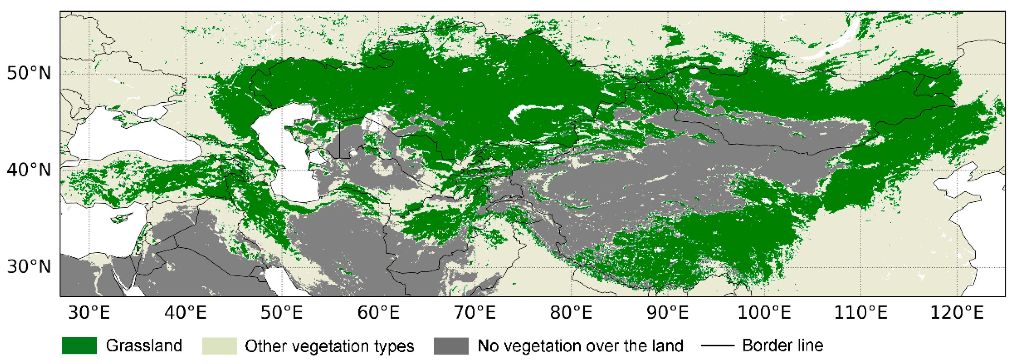
Figure 1. The study area: the Eurasian steppe. The classification followed the International Geosphere-Biosphere Program (IGBP) principle derived from Moderate Resolution Imaging Spectroradiometer (MODIS) land cover product with a 0.05° spatial resolution. Water has been masked by the color white.
Remotesensing 13 03159 g001
Figure 2. The spatial Pearson’s correlation coefficient (r) of solar-induced chlorophyll fluorescence (SIF) with precipitation (P), vapor pressure deficit (VPD), evaporative stress (ES), and root zone soil moisture (RSM). (ad) respectively represented the spatial r of SIF with P (r (SIF, P)), VPD (r (SIF, VPD)), ES (r (SIF, ES)), and RSM (r (SIF, RSM)).
Remotesensing 13 03159 g002
Figure 3. Comparison between the original time series of SIF and RSM at 50°N and 70°E and the deseasonalized time series of them. (a) represented the original time series of SIF and RSM, and (b) showed the deseasonalized time series of SIF (SIFds) and RSM (RSMds).
Remotesensing 13 03159 g003
Figure 4. The spatial Pearson’s correlation coefficient (r) and corresponding significance test (p) of deseasonalized solar-induced chlorophyll fluorescence (SIFds) with deseasonalized precipitation, vapor pressure deficit, evaporative stress, and root zone soil moisture (Pds, VPDds, ESds, and RSMds). (ad) respectively represented the spatial r of SIFds with Pds (r (SIFds, Pds)), VPDds (r (SIFds, VPDds)), ESds (r (SIFds, ESds)), and RSMds (r (SIFds, RSMds)). (eh) respectively represented the spatial p of SIFds with Pds (p (SIFds, Pds)), VPDds (p (SIFds, VPDds)), ESds (p (SIFds, ESds)), and RSMds (p (SIFds, RSMds)).
Remotesensing 13 03159 g004
Figure 5. The spatial lag phases of solar-induced chlorophyll fluorescence (SIF) to precipitation (P), vapor pressure deficit (VPD), evaporative stress (ES), and root zone soil moisture (RSM). (ad) were the spatial lag phases of SIF to P, VPD, ES, and RSM respectively.
Remotesensing 13 03159 g005
Figure 6. The spatial Pearson’s correlation coefficient extremum (re) and corresponding significance test (pe) of deseasonalized solar-induced chlorophyll fluorescence (SIFds) with deseasonalized precipitation (Pds), vapor pressure deficit (VPDds), evaporative stress (ESds), and root zone soil moisture (RSMds). (ad) respectively represented the corrected spatial r of SIFds with P (re (SIFds, Pds)), VPDds (re (SIFds, VPDds)), ESds (re (SIFds, ESds)), and RSMds (re (SIFds, RSMds)). (eh) respectively represented the spatial p of SIFds with Pds (pe (SIFds, Pds)), VPDds (pe (SIFds, VPDds)), ESds (pe (SIFds, ESds)), and RSMds (pe (SIFds, RSMds)).
Remotesensing 13 03159 g006
Figure 7. Histogram comparison between the spatial Pearson’s correlation coefficient (r) of deseasonalized solar-induced chlorophyll fluorescence (SIFds) with deseasonalized precipitation (Pds), vapor pressure deficit (VPDds), evaporative stress (ESds), and root zone soil moisture (RSMds) and that of the corrected data. (ad) were the histogram comparisons between the r of SIFds with Pds, VPDds, ESds, and RSMds and that of corrected data, respectively.
Remotesensing 13 03159 g007
Publisher’s Note: MDPI stays neutral with regard to jurisdictional claims in published maps and institutional affiliations.