Point Cloud Classification Algorithm Based on the Fusion of the Local Binary Pattern Features and Structural Features of Voxels

Abstract

Point cloud classification is a key technology for point cloud applications and point cloud feature extraction is a key step towards achieving point cloud classification. Although there are many point cloud feature extraction and classification methods, and the acquisition of colored point cloud data has become easier in recent years, most point cloud processing algorithms do not consider the color information associated with the point cloud or do not make full use of the color information. Therefore, we propose a voxel-based local feature descriptor according to the voxel-based local binary pattern (VLBP) and fuses point cloud RGB information and geometric structure features using a random forest classifier to build a color point cloud classification algorithm. The proposed algorithm voxelizes the point cloud; divides the neighborhood of the center point into cubes (i.e., multiple adjacent sub-voxels); compares the gray information of the voxel center and adjacent sub-voxels; performs voxel global thresholding to convert it into a binary code; and uses a local difference sign–magnitude transform (LDSMT) to decompose the local difference of an entire voxel into two complementary components of sign and magnitude. Then, the VLBP feature of each point is extracted. To obtain more structural information about the point cloud, the proposed method extracts the normal vector of each point and the corresponding fast point feature histogram (FPFH) based on the normal vector. Finally, the geometric mechanism features (normal vector and FPFH) and color features (RGB and VLBP features) of the point cloud are fused, and a random forest classifier is used to classify the color laser point cloud. The experimental results show that the proposed algorithm can achieve effective point cloud classification for point cloud data from different indoor and outdoor scenes, and the proposed VLBP features can improve the accuracy of point cloud classification.

1. Introduction

In recent years, with the rapid development of three-dimensional (3D) sensors, point cloud data have been widely used in fields such as unmanned driving, measurement, remote sensing, smart agriculture, “new infrastructure”, and virtual reality. In recent years, acquisition systems that can acquire point cloud data with color information, such as depth cameras and backpack/handheld mobile surveying and mapping systems, have attracted increasing attention and been widely used. The feature extraction and classification of point clouds are the key steps in point cloud data application.

In the process of constructing 3D semantic maps and performing feature extraction based on point clouds, the classification accuracy of point clouds directly affects the application effects of a method. In point cloud segmentation, classification, registration, and surface reconstruction algorithms’ processing effects mostly rely on the feature extraction ability of the method applied. The accuracy of point cloud classification is closely related to the effectiveness of features. Therefore, research on point cloud feature extraction and classification is of great significance.

For the feature extraction of point clouds, researchers proposed a large number of feature descriptors including, for example, normal vector, elevation feature [1], spin image [2], covariance eigenvalue feature [3,4], global feature viewpoint feature histogram (view feature histogram, VFH) [5], clustered view feature histogram (CVFH) [6], and fast point feature histogram [7] (fast point feature histograms, FPFH). However, the abovementioned features are all extracted from the geometric structure information of the point cloud and lack the use of the color information of the color point cloud.

Considering the point cloud data acquired in recent years usually have color information and the geometric structure characteristics of the point cloud cannot fully describe the object, it is necessary to combine the color information and the geometric structure of the point cloud for analysis. For example, for a flat point cloud area, the geometric features of the surface may be consistent. If there are important pattern marks on the plane, the geometric structure features cannot find the distinction. In contrast, the color information and texture features can capture the variation on this plane.

In addition, the color point cloud is obtained by fusing the data collected by the camera and the LiDAR sensor. Considering the fusion level is low, the original data collected by the sensor are retained to the greatest extent [8]. Achanta et al. [9] used the SLIC algorithm to combine the color similarity with the spatial neighbors of the image plane to use the color information of the reasonable color point cloud. This method uses the lab color space to represent the color features of the point cloud, combined with the pixel position, to form a five-dimensional feature vector. The feature vector uses Euclidean distance to measure the similarity between three-dimensional points. The effect of this method is unstable and sensitive to noise.

For the classification of point clouds, the traditional method is to determine the category of each point by defining relevant judgment rules. For example, by assuming the height of the ground point in the neighboring area is the smallest as the judgment rule, all ground points are marked. However, in many cases, it is difficult to design a robust decision rule and the effect is not ideal. To solve this problem, methods based on machine learning are widely used for point cloud classification. The basic idea of this kind of method is to perform feature extraction on the point cloud, use the point cloud features of the training set to train a classifier, and then use the classifier to classify the point cloud to be classified. Currently, commonly used classifiers are random forest (RF) [10], multilayer perceptron (MLP) [11], support vector machine (SVM) [12], and AdaBoost [13].

Guan [14] and others applied the random forest classifier to the feature selection of point cloud data and achieved good classification results. This also shows that the use of random forest classifiers can improve the performance of data classification [15]. Mei et al. [16] used the RGB value of each point, the normal vector of each point extracted from the neighboring points in the radius neighborhood, the spin image and the elevation feature, the boundary and label constraints for feature learning, and finally a linear classifier to classify each point. Although this type of algorithm directly integrates the three-channel value of the color into the feature of the point, it does not make full use of the color information.

To leverage point clouds’ color information, this paper draws on references to the local binary pattern feature description operator (local binary pattern, LBP) [17,18] in a two-dimensional image. The grayscale does not change with any single transformation. The degree scale has good robustness and no parameters (non-parametric). There is no need to pre-assume its distribution in the application process and then extend it to the feature description of point clouds. For a two-dimensional image, a fixed-position neighborhood can be used to construct LBP features. However, the point cloud data are irregular and disordered, and the fixed neighborhood position of each point cannot be directly obtained.

Therefore, we propose a voxel-based local binary pattern feature, that is, the VLBP feature. In addition, to achieve the effective classification of point cloud data with color information, we propose a point cloud classification algorithm based on the fusion of voxel local binary pattern features and geometric structure features in which the random forest classifier with an excellent classification performance is selected. The process of the proposed classification algorithm is shown in Figure 1.

As shown in Figure 1, the proposed algorithm first voxelizes the input point cloud data so that the neighborhood of each point is regularized. Then, the gray-level mean and gray-level variance features of each cube for each voxel constructed by a single point are extracted, and the gray information between the center of the voxel and the neighboring sub-voxels is compared to obtain the local difference. Then, local difference sign–magnitude transform (LDSMT) is performed on the local difference.

In this way, the two complementary components of the sign and magnitude of the local domain are obtained and converted into binary codes through the global thresholding of voxels. Then, the gray level at the center of the voxel is compared with the gray average of the entire voxel to obtain the global contrast. Next, the extracted VLBP features are normalized, fused with the original color RGB of the point cloud to form the color feature of the point cloud, and then fused with the geometric structure feature (normal vector and FPFH feature) of the point cloud. Finally, based on the fusion features, a random forest classifier is used to classify the point cloud. We conducted classification experiments on point clouds of different indoor and outdoor scenes to verify the effectiveness of the proposed algorithm.

The main contributions of this article are as follows:

(1)

A point cloud color feature descriptor is proposed, that is, a local binary pattern feature based on voxels (VLBP). This feature describes the local color texture information of the point cloud and has the characteristic that the grayscale does not change with any single transformation. The expression of this grayscale texture information can effectively improve the classification effect of the point cloud.

(2)

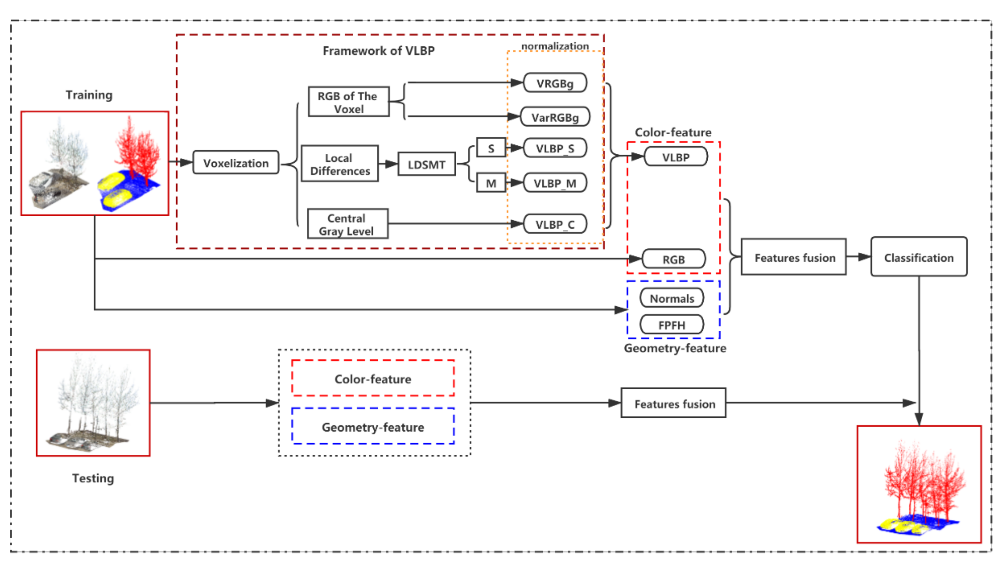
A point cloud classification algorithm based on the fusion of point cloud color and geometric structure is proposed. The proposed algorithm uses the RGB information of the color and the VLBP feature proposed in this paper as the color feature of the point cloud, merges it into the geometric structure feature of the point cloud to construct a more discriminative and robust point cloud fusion feature, and then uses a random forest classifier to effectively classify the point clouds.

2. Related Work

In this paper, the local feature VLBP of point cloud scene data based on voxel extraction is an extended texture descriptor based on the complete modeling of local binary patterns (CLBP) [19,20,21]. CLBP is a related complete binary mode scheme for texture classification that can well describe the local spatial structure of image textures. The local region is represented by its central pixel and local differential sign–amplitude transformation. The center pixels represent the gray level of the image. Through global thresholding, they are converted into binary codes, namely, CLBP_Center (CLBP_C). The local difference sign–amplitude transformation decomposes the local difference of the image into two complementary components: sign and amplitude. As shown in Figure 2, given that central pixel $g_c$ and its radius $R_s$ are circular and have evenly spaced P neighbors of $g_0,g_1,g_2,\dots ,\mathrm{and} g_{p-1}$, we can simply calculate the $d_p$ difference between $g_c$ and $g_p$. As shown in Equation (1), $d_p$ can be further broken down into two parts:

$$d_p=s_p\times m_{p}and\left\{\begin{array}{c}{s}_p=sign\left(d_p\right)\\ m_p=\left|d_p\right|\end{array}\right.$$

(1)

where $s_p=\left\{\begin{array}{c}1,d_p\ge 0\\ -1,d_p<0\end{array}\right.$ is the sign and $m_p$ is the amplitude of $d_p$. $d_p$ is the difference between the neighboring pixel and the center pixel. It cannot be used as a feature descriptor directly because the difference is sensitive to illumination, rotation, and noise. However, these effects can be overcome by dividing the difference into a sign component and an amplitude component. The two are multiplied and recorded as positive and negative binary mode CLBP_Sign (CLBP_S), and amplitude binary mode CLBP_Magnitude (CLBP_M) by Equations (2) and (3).

$$\mathrm{CLBP}\_{\mathrm{S}}_{\mathrm{P},{\mathrm{R}}_{\mathrm{s}}}={{\displaystyle \sum }}_{p=0}^{p-1}t\left(s_p,0\right)2^p$$

(2)

$$\mathrm{CLBP}\_{\mathrm{M}}_{\mathrm{P},{\mathrm{R}}_{\mathrm{s}}}={{\displaystyle \sum }}_{p=0}^{p-1}t\left(m_p,c_m\right)2^p$$

(3)

where $c_m$ is the mean value of $m_p$ in the entire image.

Equation (4) represents the global contrast CLBP_C.

$$\mathrm{CLBP}\_{\mathrm{C}}_{\mathrm{P},\mathrm{Rs}}=t\left(g_c,c_i\right)$$

(4)

where $t\left(x,c\right)=\left\{\begin{array}{c}1,x\ge c\\ 0,x<c\end{array}\right.$, $c_i$ is the average gray level of the entire image and binary encoding is performed by comparing the size of the center pixel and the pixel value of the entire image.

For a two-dimensional plane image, CLBP features can be constructed by setting the neighborhood of a fixed position. Then, for 3D irregular and disordered point cloud data, we can regularize the point cloud field by voxel and then extract the local binary pattern feature VLBP of the point cloud.

3. Voxel-Based Shading Point Cloud Feature Descriptor (VLBP)

The extraction of VLBP feature descriptors is divided into three steps: voxelization, VLBP feature descriptor construction, and voxel histogram $F_{\mathrm{VLBP}}$ feature vector, as follows.

3.1. Voxelization

Given a point $p\left(x,y,z,R,G,B\right)$ in the point cloud, we take point p as the center, use kdtree [22] to search for the radius neighbors, and find all points within radius r. All points obtained by the nearest-neighbor search are N and these N points form a cube V(r), that is, voxel V.

Then, voxel V(r) is divided into $n\times n\times n$ cubes, that is, sub-voxels. These $n\times n\times n$ sub-voxels are on the sides of the x, y, and z coordinate axes. The lengths are all equal. The side lengths of voxel V(r) in the x, y, and z directions are dx, dy, and dz, respectively. As shown in Equation (5), the side lengths of each sub-voxel in the x, y, and z directions are $L_x$, $L_y$, and $L_z$, respectively:

$$\left\{\begin{array}{c}{L}_x=dx/n\\ L_y=dy/n\\ L_z=dz/n\end{array}\right.$$

(5)

Traverse all points in voxel V(r) to determine to which sub-voxel they belong. Taking a point $q\left(x^{\prime },y^{\prime },z^{\prime },R^{\prime },G^{\prime },B^{\prime }\right)$ in V(r) as an example, find which sub-voxel this point belongs to. First, number $n\times n\times n$ as sub-voxels. Each sub-voxel is represented by coordinates (a, b, c), where $a,b,c ϵ\left[1,n\right]$. The coordinates of the sub-voxel where point q is located $\left(a_0,b_0,c_0\right)$ are shown in Equation (6):

$$\left\{\begin{array}{c}{a}_0=ceil\left(fabs\left(x^{\prime }-x_0\right)/rx\right)\\ b_0=ceil\left(fabs\left(y^{\prime }-y_0\right)/ry\right)\\ c_0=ceil\left(fabs\left(z^{\prime }-z_0\right)/rz\right)\end{array}\right.$$

(6)

where $x_0, y_0$, and $z_0$ are the minimum values of the N points in voxel V in the x, y, and z-axes direction.

The number of points contained in the i voxel is $K_i$ and the points in the i-th voxel are expressed as $P_i$= {$p_1$,$p_2$...,$p_{K_i}$}. If the number of points in the i voxel is $K_i>0$, then the $R_i,G_i, a\mathrm{nd} B_i$ values of the i-th small block are calculated by Equation (7).

$$\left\{\begin{array}{c}{R}_i=\left({{\displaystyle \sum }}_{j=1}^{K_i}{r}_j\right)/K_i\\ G_i=\left({{\displaystyle \sum }}_{j=1}^{K_i}{g}_j\right)/K_i\\ B_i=\left({{\displaystyle \sum }}_{j=1}^{K_i}{b}_j\right)/K_i\end{array}\right.$$

(7)

where $r_j,g_j$, and $b_j$ are the R, G, and B values of the j-th point, respectively. If the number of points of the i-th small block is $K_i=0$, then $R_i=G_i=B_i=0$.

The gray value ${\mathrm{Vg}}_{\mathrm{c}}$ of the voxel center is calculated by Equation (8).

$${\mathrm{V}}_{{\mathrm{g}}_{\mathrm{c}}}=R\times 0.299+G\times 0.587+B\times 0.114$$

(8)

The average gray value Vg_i of the i-th sub-voxel in voxel V is calculated by Equation (9).

$${Vg}_c=\frac{{{\displaystyle \sum }}_{j=1}^{K_i}\left(R_j\times 0.299+G_j\times 0.587+B_j\times 0.114\right)}{K_i}$$

(9)

The gray value of the center point p of the current voxel is ${Vg}_c$, the gray values of adjacent sub-voxels in voxel $n\times n\times n-1$ are $V{g}_i$, and i represents the i-th small block.

The abovementioned voxelization on all points in the point cloud are performed and the gray values of the current voxel center point p and its adjacent voxels can be calculated. Then, the VLBP feature descriptor of voxels is constructed.

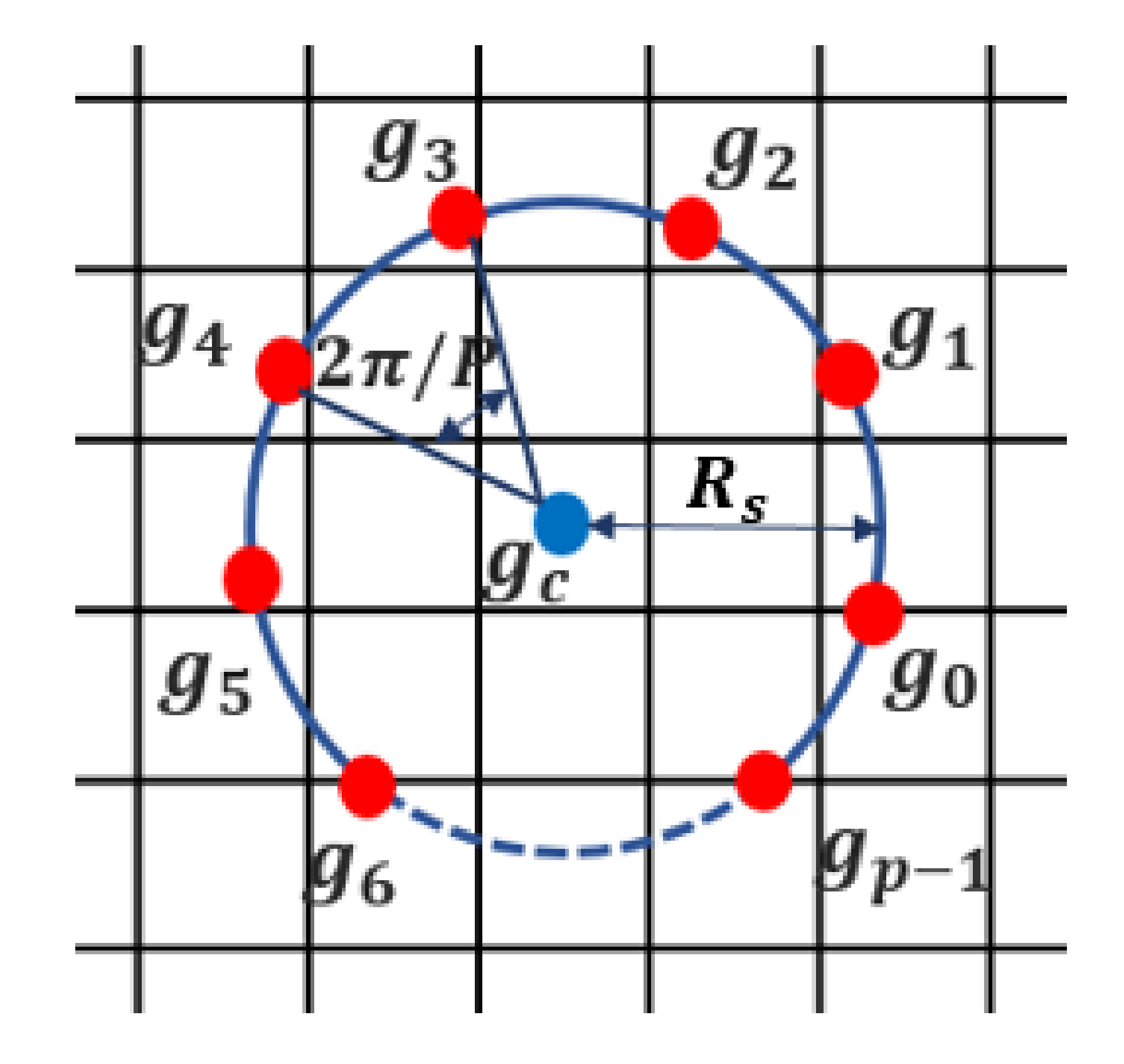
3.2. VLBP Descriptor Construction

The gray value of the current point (the sub-voxel where the current point is located) p is $g_c$ and the gray values of the $\left(n\times n\times n-1\right)$ neighborhood blocks of this point in the voxel are $g_i$, representing the i-th small block, i = 0,1...$\left(n\times n\times n-1\right)-1$. The grayscale difference between the i-th small block and the small block where the current point is located is $d_i=g_i-g_c$. Using Equation (1) in VLBP, d_i is further divided into two components according to Equation (10): sign component, $s_i$, and amplitude component, $m_i$.

$$d_i=s_i\times m_i$$

(10)

Among them $\mathrm{are}\left\{\begin{array}{c}{s}_i=sign\left(d_i\right)\\ m_i=\left|d_i\right|\end{array}\right.$ and $s_i=\left\{\begin{array}{c}1,d_i\ge 0\\ -1,d_i<0\end{array}\right.$

In VLBP, a local area is represented by its central pixel and local differential sign–amplitude transformation (LDSMT). The gray level of the central voxel is simply encoded with a binary code after global thresholding. LDSMT decomposes the local structure within the voxel into two complementary components: difference sign and difference amplitude. The three-dimensional features of VLBP are VLBP_S, VLBP_M, VLBP_C, and I = (n × n × n − 1). These three-dimensional features are defined as Equation (11).

$$\left\{\begin{array}{l}\mathrm{VLBP}\_{\mathrm{S}}_I={{\displaystyle \sum }}_{i=0}^{I-1}t\left(s_i,0\right)2^i \\ VLBP\_M_I={{\displaystyle \sum }}_{i=0}^{I-1}t\left(m_i,c_m\right)2^i\\ \mathrm{VLBP}\_{\mathrm{C}}_I=t\left(g_c,c_n\right)\end{array}\right.$$

(11)

where $t\left(x,c\right)=\left\{\begin{array}{c}1,x\ge c\\ 0,x<c\end{array}\right.$ is the comparison function; $c_m$ is the mean value of n × n × n − 1 $m_i$ of the entire voxel, that is, $c_m=\left({{\displaystyle \sum }}_{i=0}^{I-1}{m}_i\right)/I$; and $c_n$ is the average gray value of n × n × n sub-voxels in the entire voxel, that is, $c_n=({{\displaystyle \sum }}_{i=0}^{I-1}{m}_i+g_c)/\left(n\times n\times n\right)$.

3.2.1. Scale Invariance

To make VLBP descriptors scale-invariant, two different scales are selected for voxelization and then the VLBP descriptor is constructed. By changing the size of r, voxels of different scales are obtained. The features of different scales obtained are directly output in order, which can make the features more robust [20].

3.2.2. Rotation Invariance

When constructing voxels, this article numbered n × n × n sub-voxels. They were numbered based on XYZ, XZY, YXZ, YZX, ZXY, and ZYX as 6 different coordinate directions and then these numbers were placed in ascending order. Arrange and extract the values of VLBP_S and VLBP_M in the voxel, in turn, and then encode it, that is, construct a binary code structure similar to 1001111000 … 00. Then, convert the binary arrangement to the decimal number to find the smallest one. The 0–1 binary obtained after the rotation sorting is performed according to the finally obtained 01 binary in the definition formulas of $\mathrm{CLBP}\_S_I$ and $\mathrm{CLBP}\_M_I$.

3.3. F_VLBP Feature Vector of Voxel Histogram

The construction steps of the LBP feature vector of the voxel histogram are as follows:

• Given search radius r₂, take point p as the search center point and use kdtree as the search radius to perform a second radius near-neighbor search to find all points within its radius, r₂.
• Find the VLBP_S and VLBP_M values corresponding to all points obtained by this radius neighbor search, divide $0–2^I$ into the ${\mathrm{T}}_{\mathrm{ZN}}$ detection interval, and then calculate the VLBP_S and VLBP_M values corresponding to each point. Here, ${\mathrm{T}}_{\mathrm{ZN}}$ is a threshold to divide the feature value interval for the histogram statistics. The following also pertain to the test interval:
• After traversing all points, record the number of times in the ${\mathrm{T}}_{\mathrm{ZN}}$ interval and create two new ${\mathrm{T}}_{\mathrm{ZN}}$-dimensional features: VLBP_S(r) and VLBP_M(r). Replace VLBP_S and VLBP_M with these two new features.
• The final VLBP characteristics of each voxel are:

  $$F_{VLBP}=\left[V{\left(r\right)}_{RGBg},Var{\left(r\right)}_{RGBg},VLB{P}_{S\left(r\right)},VLB{P}_{M\left(r\right)},\mathrm{and}VLB{P}_{C\left(r\right)}\right].$$

  (12)

  Among them, VRGBg is the average value of the gray value of the R, G, and B structure of the N points in voxel V. VarRGBg is the variance of the gray value constructed by R, G, and B of N points in voxel V.
• Traverse all points in the point cloud and generate a VLBP feature for each point; change radius r of the first-radius nearest-neighbor search; and generate a set of VLBP features again and continue writing. Repeat this step until the radius set by the scale invariance is reached.

4. Point Cloud Classification Based on Multifeature Fusion and Random Forest

Point cloud classification based on multifeature fusion and random forest is divided into two steps (multifeature fusion and the use of random forest to classify point clouds) as follows:

4.1. Multifeature Fusion

To improve the characterization ability and robustness of point cloud features, this paper fuses the point cloud color RGB, normal vector feature, and FPFH feature with the VLBP feature constructed in this paper. The feature corresponding to each point in the point cloud after fusion is $F=\left[F_{VLBP},F_{RGB},F_{Normal},F_{FPFH}\right]$. Among them, the 10-dimensional VLBP feature $F_{VLBP}$ constructed in this paper and the 3-dimensional original point cloud color RGB constitute the color feature of the point cloud. The 3-dimensional normal feature $F_{Normal}$ and the 33-dimensional fast feature histogram feature $F_{FPFH}$ constitute the geometric structure feature of the point cloud.

Among them, the normal vector feature $F_{Normal}$ estimates the neighborhood plane of each point in the original point cloud and the feature vector corresponding to the smallest feature value obtained by PCA is regarded as the normal feature of the point. $F_{FPFH}$ is used to describe the relationship between the adjacent points of the point cloud, has the advantages of low computational complexity and strong robustness, and has better results when used for point cloud classification. After multifeature fusion, feature F of each point in the original point cloud has 49 dimensions (the 10-dimensional features are VLBP features obtained at two different scales).

4.2. Point Cloud Classification

The proposed method adopts a classification strategy based on a single point of the point cloud; that is, after the fusion feature construction of each point of the point cloud is completed, each point in the point cloud is classified by a machine learning classifier. The random forest classifier is suitable for multi-classification problems, can handle high-dimensional input features, has good classification performance in the point cloud classification of indoor and outdoor scenes, and can achieve high classification accuracy. Therefore, we choose random forest classifiers to perform point cloud classification. Among them, the random forest constructed in this paper has 250 trees and the maximum tree depth is 20.

5. Analysis of Experimental Results

To evaluate the effectiveness of the proposed algorithm, we conduct experiments on three mobile laser scanning (MLS) urban point cloud scenes and two indoor point cloud scenes, and perform qualitative and quantitative analyses.

5.1. Experimental Data

In this paper, five different point cloud scenarios are selected to verify the proposed algorithm and the point cloud data all contain x, y, z, R, G, and B information, i.e., point coordinates and color information. Collection equipment of a point cloud scene is shown in Figure 3. Scene 1, Scene 2, and Scene 3 are outdoor scene colored point cloud data collected by advanced backpack mobile surveying and mapping robots provided in CSPC-Dataset [23]. The robot collects the data of these scenes by laser sensors and panoramic cameras, and the average point cloud density is about 50~60/m². After the refined modeling and coloring of point clouds, the complete colored point cloud of the scene can be produced. The dataset contains both larger objects (e.g., buildings, ground, and trees) and smaller objects (e.g., cars). Scene 4 and Scene 5 are indoor scene point clouds, which are chosen from the S3DIS dataset [24]. The S3DIS dataset is an indoor point cloud dataset produced and developed by Stanford University et al. with a Matterport camera (combined with three structured light sensors with different spacings). The dense point cloud obtained in this dataset has high precision and uniform color distribution. The Scene 4 and Scene 5 produced in this paper include four types of objects, i.e., chair, table, ground, and potted plants. The training set and test set of the five scenarios are shown in Figure 4, Figure 5, Figure 6, Figure 7 and Figure 8.

Table 1. Statistics of experimental datasets.

	Train				Test
	Floor	Building	Car	Tree	Floor	Building	Car	Tree
Scene 1	54.327		29.523	46.068	25.038		63.174	93.852
Scene 2	71.587	123.521	10.545	28.754	29.080	46.854	5918	7248
Scene 3	119.255	180.919	15.394	13.504	155.931	201.930	17.492	87.601
	Chair	Table	Floor	Flower	Chair	Table	Floor	Flower
Scene 4	24.025	17.671	77.880		24.713	29.467	74.692
Scene 5	30.801	16.148	62.596	18.394	28.748	14.611	47.662	19.278

shows the distribution of the exact number of points for training and the test sets for each scene.

The proposed algorithm is implemented on PCL1.8.1 (C++), python3.7.6, and CloudCompare2.11.3. All experiments in this article are run on a computer with an AMD Ryzen 5 3600 6-core processor at 3.59 GHz with 16 GB of RAM. The average training time of five scenes is about 6.48 min, and the average testing time of five scenes is 3.96 min. To evaluate the performance of the different algorithms more comprehensively and effectively, we uses Precision/Recall/F1-scores to evaluate the classification effect of each category, and uses Overall Accuracy (OA) and Kappa to evaluate the overall classification result of each scene. These evaluation indicators reflect the classification effects of different attributes. The higher the values of these classification indicators, the better the classification effect, as shown in

Table 2. Definition relationships between predicted and true values.

Ground Truth	Predicted
	Positive	Negative
Positive	True Positive (Tp)	False Negative (Fn)
Negative	False Positive (Fp)	True Negative (Tn)

from which T_p, F_n, F_p, and T_n represent the number of true positives, false negatives, false positives, and true negatives.

Precision measures the ability of a classifier to not mistakenly divide real negative samples into positive ones. The calculation method is Equation (13).

$$precision=\frac{T_p}{T_p+F_p}$$

(13)

Equation (14) is the calculation method of Recall, Recall measures the ability of a classifier to find all positive samples.

$$recall=\frac{T_p}{T_p+F_n}$$

(14)

In order to comprehensively evaluate the classification ability of a classifier for each category, the F1 score is usually used to measure the whole classifier. The calculation method is Equation (15).

$$F_1-score=\frac{2\times precision\times recall}{precision+recall}$$

(15)

The experiment point cloud dataset has multiple category labels. Therefore, to comprehensively evaluate the classification effect of the algorithms on all categories of the whole point cloud, we use OA and Kappa to evaluate the overall classification performance of different algorithms. Each evaluation metric is calculated according to Equations (16)–(18).

$$\mathrm{OA}=\frac{{{\displaystyle \sum }}_{i=1}^L{C}_{ii}}{{{\displaystyle \sum }}_{j=1}^L{{\displaystyle \sum }}_{k=1}^L{C}_{jk}}$$

(16)

$$\mathrm{Kappa}=\frac{\mathrm{OA}-P_e}{1-P_e}$$

(17)

$$p_e=\frac{\left({{\displaystyle \sum }}_{j=1}^L{{\displaystyle \sum }}_{i=1}^L\left(C_{ij}\times C_{ji}\right)\right)}{Q\times Q}$$

(18)

where C is a $L\times L$ classification confusion matrix; L is the number of an object category; $C_{ij}$ is the true label of the i-th class classified to the j-th class; and Q is the number of all points.

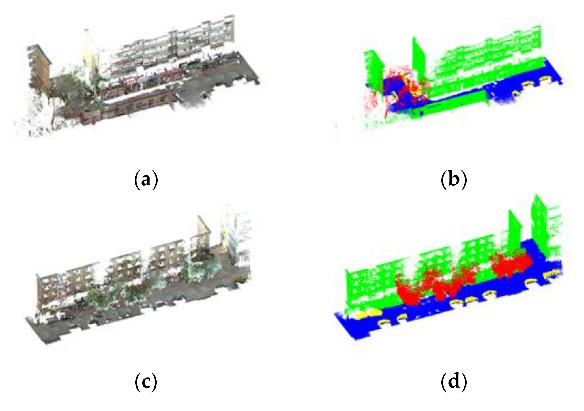
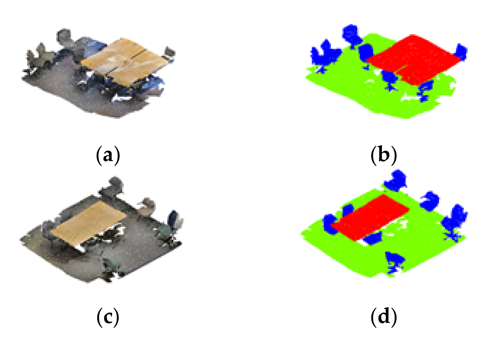
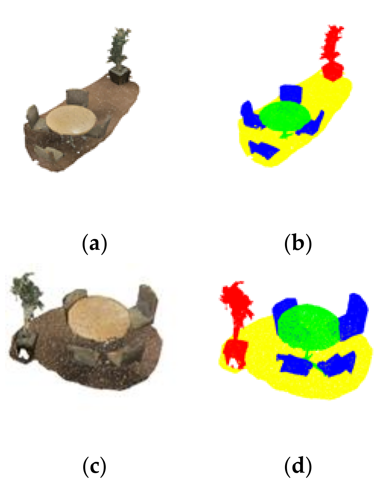
5.2. Point Cloud Classification Effect

To evaluate the effect of the proposed algorithm and verify the influence of different classifiers and point cloud features on point cloud classification, this paper compares the proposed algorithm with other classification algorithms composed of point cloud features and classifiers. The features, classifiers, and classification accuracy of the experimental comparison methods are listed in Table 2. The classifiers include the random forest classifier (RF main parameters: 250 forest trees; the maximum tree depth is 20), multilayer perceptron classifier (MLP main parameters: a hidden layer with 100 neurons; the activation function is relu; regular term parameter alpha = 20; etc.), and support vector machine classifier (SVM main parameters: error term penalty coefficient C = 1; kernel = ‘rbf’; etc.). We also compared with PointNet [25], which is a deep learning method based on a multilayer perceptron.

The features include the following: based on point cloud color extraction feature $F_{\mathrm{VLBP}}$ and point cloud geometric structure feature $F_{N\_F}$ (normal vector and fast feature histogram feature), the $F_{N\_F\_RGB}$ feature refers to the RGB color information integrated on the basis of feature $F_{N\_F}$. Feature $F_{\mathrm{All}}$ is a fusion of the color features of the point cloud (RGB and VLBP features) and point cloud geometric structure feature $F_{N\_F}$.

From the results listed in

Table 3. Comparison of the Kappa/OA value (%) of each point cloud scene under different classifiers and feature conditions. For each scene, bold font indicates the best result of each classifier.

Classifiers	Features	Scene 1	Scene 2	Scene 3	Scene 4	Scene 5
RF	$F_{VLBP}$	51.9/73.8	32.0/53.6	33.8/55.7	43.3/71.0	45.7/65.8
	$F_{N\_F}$	84.0/90.7	79.1/87.6	73.0/82.9	81.9/90.9	82.5/88.0
	$F_{N\_F\_RGB}$	85.7/91.4	79.1/87.7	73.6/83.3	91.4/95.9	84.4/88.1
	$F_{\mathrm{All}}$	86.8/92.1	79.4/87.9	73.2/83.1	94.4/97.0	84.6/89.5
MLP	$F_{VLBP}$	56.7/75.7	32.1/52.5	36.7/55.5	42.4/69.5	36.8/51.2
	$F_{N\_F}$	79.0/86.4	60.8/73.5	57.4/73.3	72.9/82.8	78.2/84.5
	$F_{N\_F\_RGB}$	84.9/90.5	51.4/69.5	60.8/71.8	74.0/84.9	78.0/85.1
	$F_{\mathrm{All}}$	85.8/91.4	63.5/78.4	57.7/73.7	88.1/94.0	81.1/86.0
SVM	$F_{VLBP}$	57.0/75.6	34.1/52.4	32.8/43.8	35.6/70.2	36.8/52.8
	$F_{N\_F}$	80.0/88.0	53.9/73.3	52.0/70.0	74.5/85.7	79.2/85.7
	$F_{N\_F\_RGB}$	84.5/91.1	54.2/73.4	53.1/70.5	77.1/84.9	79.5/87.3
	$F_{\mathrm{All}}$	85.0/90.7	55.6/74.2	56.5/73.5	90.8/95.3	83.5/88.6
PointNet	Deep feature	62.1/76.3	54.2/61.4	57.7/74.9	58.7/82.9	50.8/61.2

, we can make the following observations:

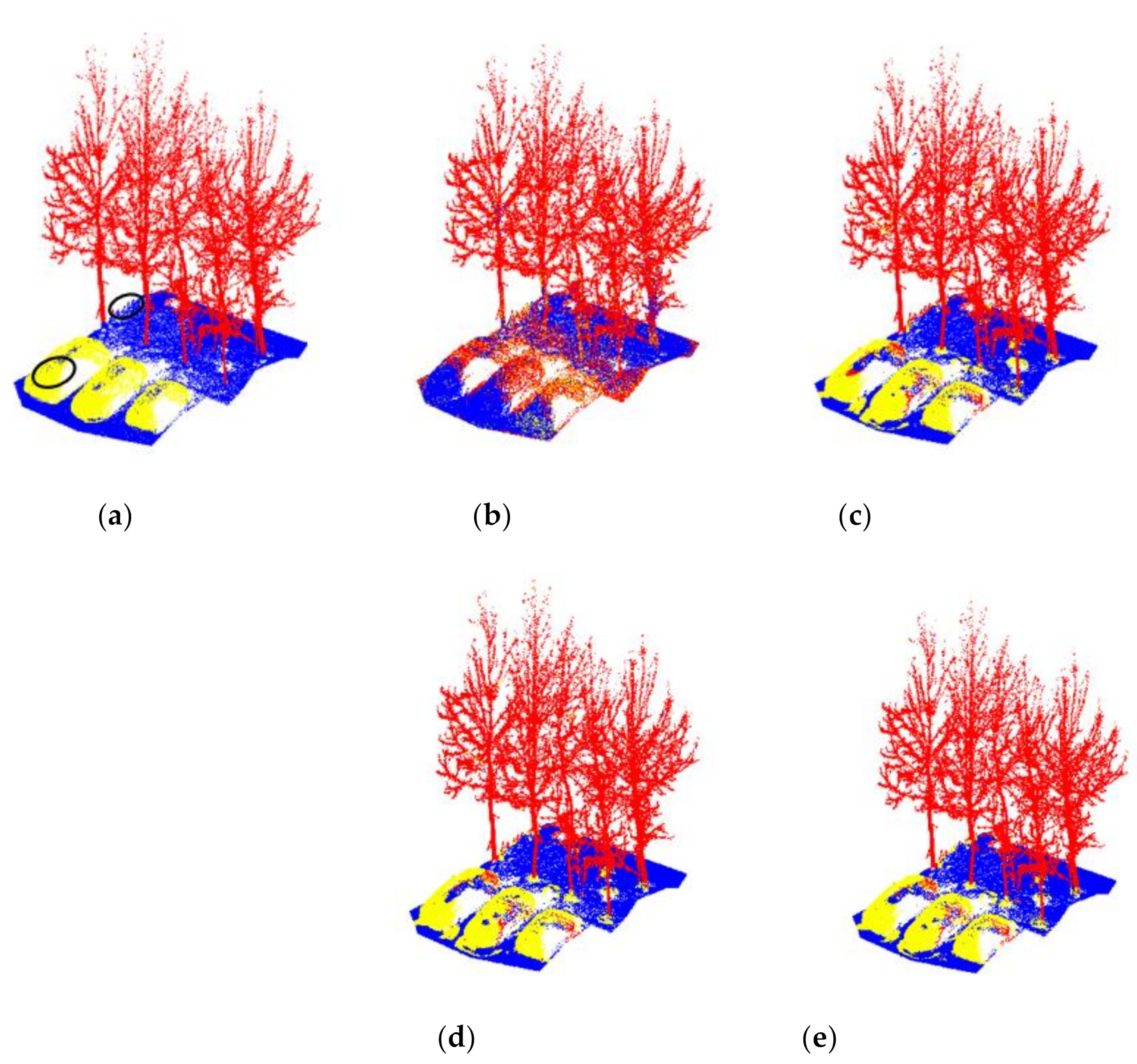
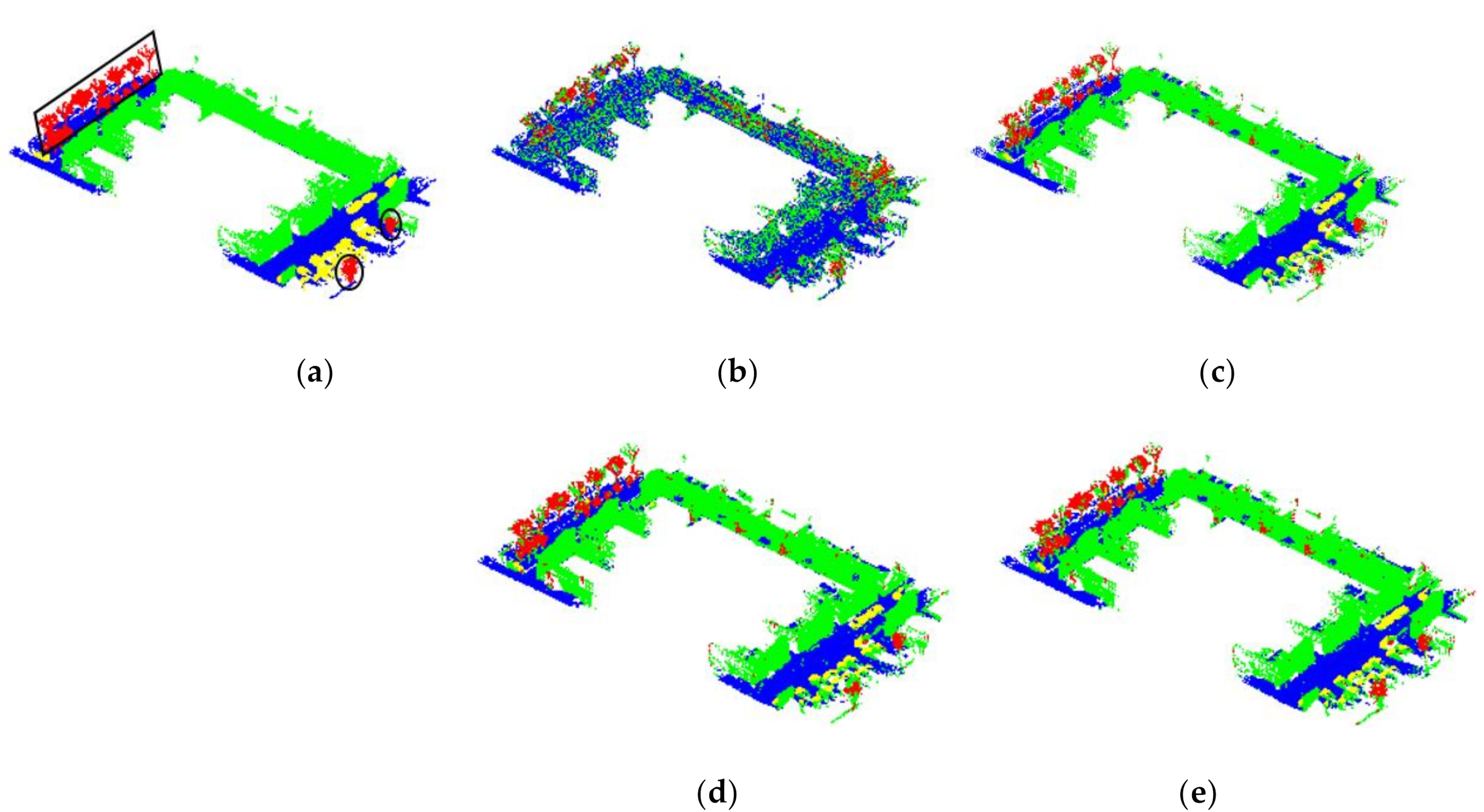
• From the data in the table, we can see that the classification accuracy (Kappa/OA) of the proposed algorithm is different in different scenarios, but the point cloud classification accuracy is basically the highest in all feature fusion situations and the results of the five scenarios are in different features. The results’ trends of the classifier is consistent.
• By comparing the results of five scenes of point cloud classifications using different types of classifiers for the same feature, it can be seen that the features used in the proposed method can achieve the best classification results by using random forest classifiers; that is, the classification algorithm designed in this article is better than that based on other classifications.
• A comparison of the effects of classifying different types of features by the same classifier shows that, based only on the VLBP features proposed in this paper, they cannot achieve better classification results because the feature descriptors proposed in this paper only represent the point cloud color information and lack the structural information of the point cloud. The fusion of RGB color information on the basis of geometric features will significantly improve the classification effect of point clouds. On this basis, continuing to integrate the VLBP features extracted in this paper based on color will improve the classification accuracy of point clouds.

Regardless of which classifier is used, the classification effect of the four types of feature fusion is better than the classification effect based on a single feature. This shows that the fusion of color information based on the geometric structure characteristics of the point cloud can improve the classification accuracy of the point cloud.

4.

By comparing the improvement of the classification accuracy of each scene, we can see that the RGB and VLBP color features are combined on the basis of the geometric structure characteristics of the point cloud, and the classification accuracy of indoor Scene 4 and 5 is more obvious than that of outdoor Scenes 1–3. This is because the coloring of the point cloud is not only related to the point cloud collection equipment but it is also affected by the illumination to a certain extent. This makes the coloring of the point cloud collected indoors more uniform than the point cloud collected outdoors. Thus, compared with outdoor scenes, the classification accuracy of indoor scenes is better.

In order to highlight the advantages of the random forest classifier selected in this paper, classification comparison experiments are carried out under the conditions of different features and classifiers. As shown in

Table 4. Statistics of average running time under the condition of different features and classifiers.

Feature	Average Time (min)
FVLBP	2.86
FRGB	0.58
FNormal	1.73
FFPFH	1.47
Classifier	Average Time (min)
RF	3.80
MLP	5.03
SVM	16.3
PointNet	145.86

, the average running time of $F_{\mathrm{VLBP}}$, original color feature ($F_{\mathrm{RGB}}$), normal vector feature $F_{\mathrm{Normal}}$), and fast feature histogram feature ($F_{\mathrm{FPFH}}$) of the point cloud in the five scenarios are 2.86 min, 0.58 min, 1.73 min, and 1.47 min, respectively. The average running time (i.e., the training time and test time) of the random forest classifier, the MLP classifier, and the SVM classifier are 3.80 min, 5.03 min, and 16.3 min, with the fusion features ($F_{\mathrm{VLBP}}$, $F_{\mathrm{RGB}}$, $F_{\mathrm{Normal}}$, and $F_{\mathrm{FPFH}}$). It takes an average of 145.86 min to classify the point cloud with PointNet (including 143.76 min for training and 2.1 min for testing). The random forest classifier is not only excellent in the classification effect but also excellent in time efficiency; thus, the random forest classifier is selected to classify the extracted fusion features.

To show the classification effect of the proposed algorithm more prominently, this paper compares the classification algorithms of different feature constructions using the random forest classifier. As shown in

Table 5. Comparison with the four methods in terms of “Feature Expression”.

Method	Feature	Dimension
Method 1	FVLBP	10
Method 2	FNormal + FFPFH	36
Method 3	FNormal + FFPFH + FRGB	39
Our Method	FNormal + FFPFH + FRGB + FVLBP	49

, Method 1 is a prediction classification method based on $F_{\mathrm{VLBP}}$ features and Method 2 is a prediction classification based on geometric features (i.e., normal vector and FPFH features). Method 3 is a type of predictive classification based on ${\mathrm{F}}_{\mathrm{N}\_F\_\mathrm{RGB}}$ features. Our method is a combination of point cloud color features (RGB and VLBP features) and point cloud geometric structure features (normal vector and FPFH features) for predictive classification.

As shown in

Table 6. Comparison of the classification effects of ground objects and ground objects in each scene with precision/recall/F₁-scores. For each scene, bold font indicates the best results of each metric.

	Method	Floor	Car	Tree	Building	Kappa (%)	OA (%)
Scene 1	Method 1	0.71/0.71/0.71	0.27/0.12/0.17	0.80/0.92/0.86		51.9	73.8
	Method 2	0.96/0.81/0.88	0.68/0.84/0.75	0.95/0.99/0.97		84.0	90.7
	Method 3	0.96/0.82/0.88	0.69/0.85/0.76	0.96/0.99/0.98		85.7	91.4
	Our	0.96/0.83/0.89	0.70/0.87/0.77	0.97/1.00/0.98		86.8	92.1
Scene 2	Method 1	0.47/0.82/0.60	0.22/0.06/0.09	0.39/0.31/0.35	0.68/0.46/0.60	32.0	53.6
	Method 2	0.91/0.88/0.90	0.87/0.55/0.68	0.79/0.73/0.76	0.87/0.94/0.90	79.1	87.6
	Method 3	0.91/0.88/0.90	0.89/0.55/0.68	0.80/0.74/0.77	0.87/0.94/0.90	79.1	87.7
	Our	0.91/0.89/0.90	0.89/0.57/0.69	0.82/0.75/0.77	0.87/0.94/0.90	79.4	87.9
Scene 3	Method 1	0.71/0.51/0.59	0.11/0.02/0.03	0.60/0.06/0.12	0.51/0.86/0.64	33.8	55.7
	Method 2	0.99/0.91/0.95	0.80/0.30/0.43	0.92/0.45/0.60	0.73/0.98/0.84	73.0	82.9
	Method 3	0.99/0.91/0.95	0.45/0.28/0.34	0.93/0.53/0.68	0.74/0.95/0.83	73.6	83.3
	Our	0.99/0.91/0.95	0.58/0.29/0.38	0.92/0.48/0.63	0.73/0.96/0.83	73.2	83.1
	Method	Chair	Table	Floor	Flower	Kappa (%)	OA (%)
Scene 4	Method 1	0.30/0.20/0.24	0.72/0.37/0.49	0.78/0.95/0.86		43.3	71.0
	Method 2	0.89/0.99/0.94	0.69/0.80/0.74	0.98/0.91/0.94		81.9	90.9
	Method 3	0.90/0.99/0.94	0.90/0.89/0.89	0.99/0.97/0.98		91.4	95.9
	Our	0.90/0.99/0.94	0.97/0.90/0.93	0.99/0.98/0.99		94.4	97.1
Scene 5	Method 1	0.53/0.33/0.41	0.67/0.55/0.60	0.69/0.87/0.77	0.66/0.71/0.68	45.7	65.8
	Method 2	0.89/0.77/0.83	0.79/0.75/0.77	0.92/0.97/0.94	0.83/0.92/0.88	82.5	88.0
	Method 3	0.90/0.78/0.83	0.82/0.80/0.82	0.94/0.98/0.96	0.82/0.92/0.88	84.4	88.1
	Our	0.90/0.78/0.83	0.83/0.80/0.82	0.94/0.98/0.96	0.84/0.93/0.88	84.6	89.5

, the comparison of five point cloud scenes classification results are given.

From the results listed in Table 6, it is easy to draw the following conclusions below:

(1)

From the comparison of each metric, we can see that the proposed classification algorithm achieved 86.8/92.1%, 79.4/87.9%, 73.2/83.1%, 94.4/97.1%, and 84.6/89.5% classification Kappa/accuracy in the five scenarios. Considering all evaluation indicators, the proposed algorithm has advantages over both the algorithm without color features (Method 2) and the algorithm with RGB features (Method 3).

(2)

A comparison of the four algorithms shows that Method 3 introduces RGB based on the geometric structure characteristics of the point cloud and improves the classification effect of each scene by 0.7%, 0.1%, 0.4%, 5.0%, and 0.1%. The proposed algorithm integrates RGB and VLBP features based on geometric structure features, and the fusion features increase the classification accuracy of each scene by 1.4%, 0.3%, 0.2%, 6.2%, and 1.5%, respectively. This shows that the four fusion features are more discriminative to the point cloud representation, which improves the classification effect. The proposed algorithm can achieve better point cloud classification on the point cloud data of different scenes and the proposed VLBP feature can improve the point cloud classification.

(3)

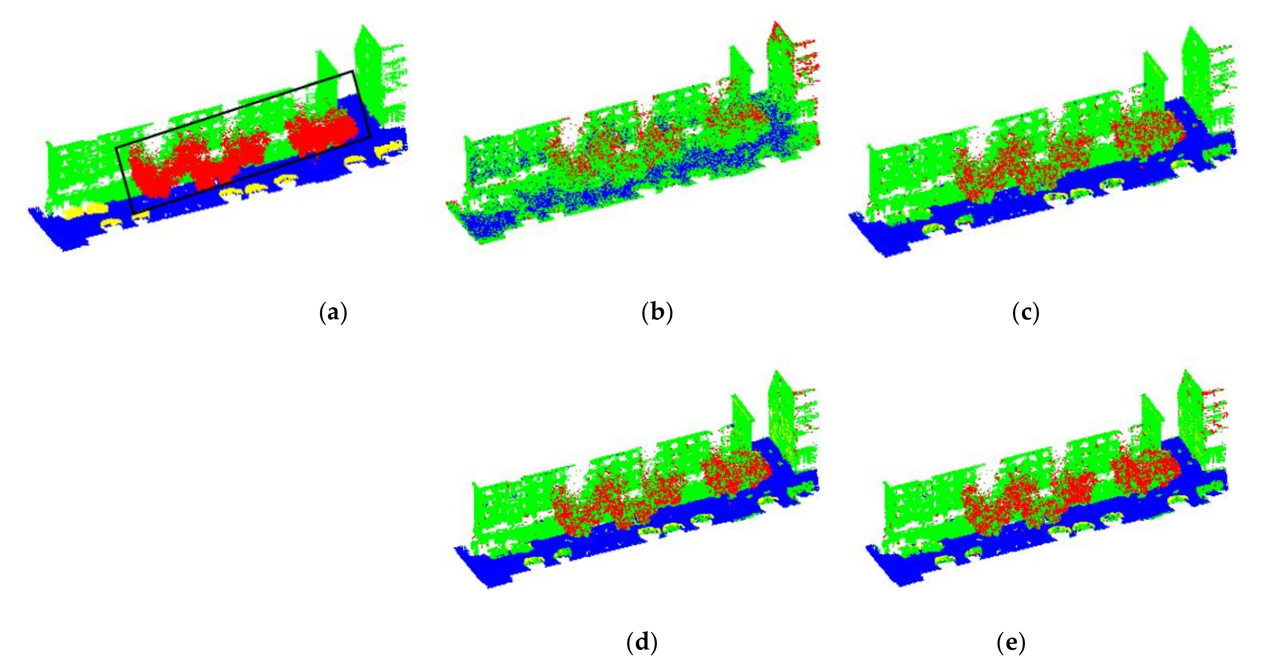
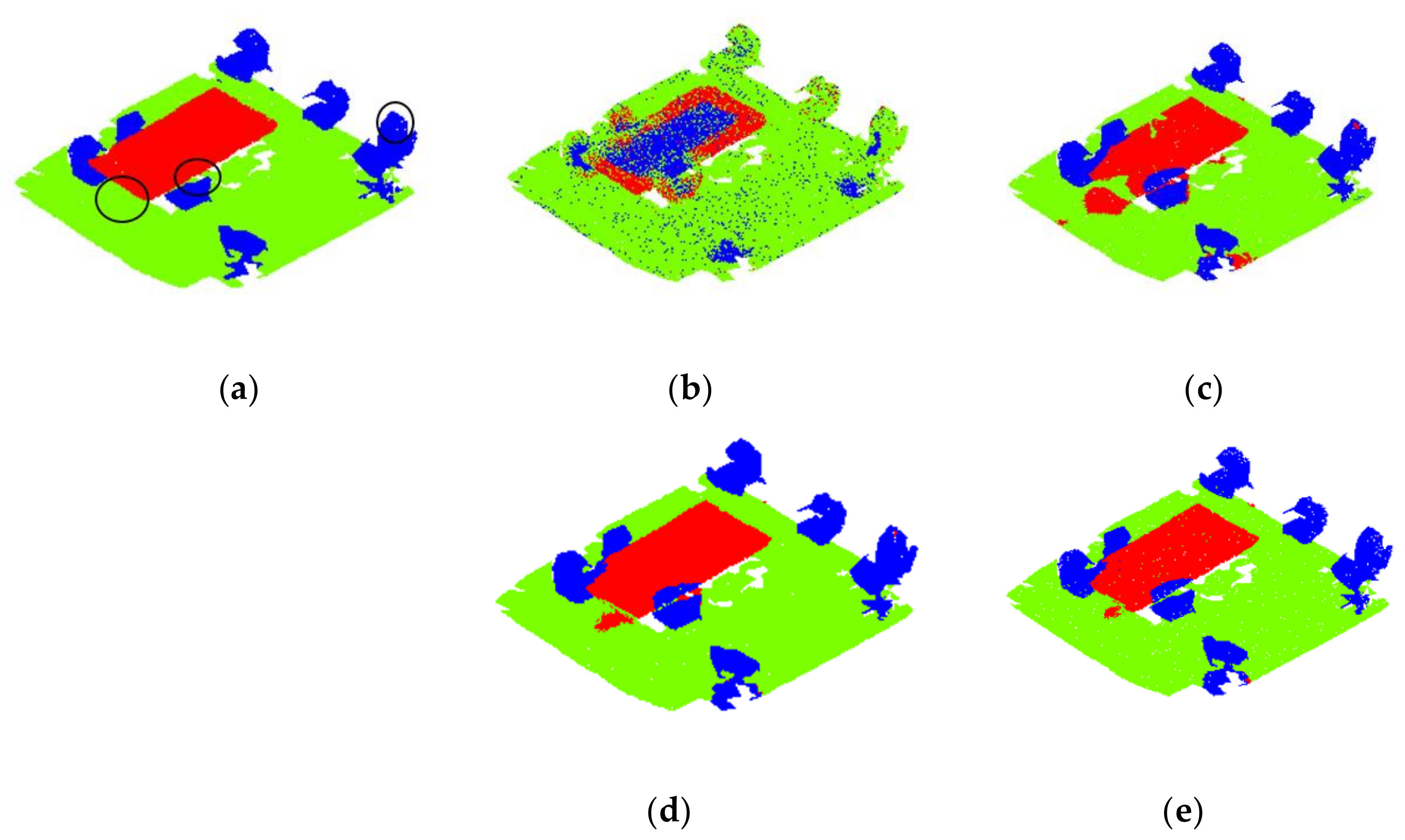
From the comparison in Table 3, it can be seen that Method 3 shows significant improvements for most indicators compared to Method 1 and Method 2, especially in Scene 4 and 5, and the classification effect is significantly improved. This shows that the point cloud color feature has an improved effect on point cloud classification. From a comparison between Method 3 and the algorithm in this paper, it can be seen that in the outdoor Scenes 1–3, the algorithm in this paper performs better than Method 3 in most cases. It can be seen that in the indoor Scene 4 and 5, the algorithm in this paper shows a significant improvement for all indicators compared to Method 3. This also shows that in the case of less noise in the color information of the point cloud coloring, the VLBP feature descriptor proposed in this paper can significantly improve the point cloud classification effect.

(4)

By observing Scene 4 and the other four scenes, we can see that the proposed method has the best classification performance on the point cloud scene containing only man-made objects. When there are irregular objects such as plants in the scene, it will increase the complexity of the scene, thereby reducing the classification performance. It can be seen from the precision/recall/F₁-scores in Table 6 that the performance of the proposed method for the vast majority objects has a certain improvement. Especially for the indoor point clouds, the improvement is more significant. This is because the color information of the indoor point cloud is more accurate than the outdoor point clouds, which is caused by the colored point cloud collection device.

In this paper, the proposed method has been compared with other methods by multiple evaluation metrics at the same time. Considering the time efficiency, it can be seen from Table 4 that the proposed method outperforms PointNet. For the Kappa and OA, the proposed method can achieve better performance than the other methods with different features and classifiers. Therefore, we can make the satisfactory conclusion that the overall performance of the proposed classification method is a promising method by considering different evaluation metrics and ablation studies.

To show the point cloud classification effect of the algorithm in this paper more intuitively, Figure 9, Figure 10, Figure 11, Figure 12 and Figure 13 show the classification effect of different algorithms on five point cloud scenes. It can be seen from the figure that the classification result of the algorithm in this paper is closest to the true value effect and the classification effect of trees in Scenes 1–3 is better than that of other algorithms. According to a comparison of (b) and (c) in Figure 9, Figure 10, Figure 11, Figure 12 and Figure 13, the classification based on VLBP features and the classification based on the normal vector and FPFH features will have a certain complementary effect. After the fusion of RGB and VLBP features, for Scene 2 and Scene 3, which are medium and small scenes, some building points are misclassified as tree points, some table points and chair points in Scene 4 are misclassified, and potted plants and chairs in Scene 5 are misclassified. This confusion is caused by the similar colors in the point cloud but the overall classification effect is generally good.

In this article, Scenes 1–3 are outdoor point cloud scenes. As shown in Figure 9, Figure 10 and Figure 11 (the black circles/boxes in the figure), the proposed algorithm has obvious advantages but the difference between the proposed algorithm and Method 3 is relatively small. This is because in outdoor scenes, as shown in Figure 4, Figure 5 and Figure 6, the color information corresponding to the color point cloud has certain noise and errors, making the effect of the proposed VLBP feature descriptor not obvious. However, Scene 4 and Scene 5 are indoor scenes based on the color point cloud data collected by a Kinect, as shown in Figure 7 and Figure 8. The color information is relatively stable and there is less noise. As shown in Figure 12 and Figure 13 (the black circle/box), the algorithm proposed in this paper has obvious advantages over other algorithms. Although Method 3 also uses color features, the effect is still not as good as the algorithm in this paper. This also shows the effectiveness of the VLBP feature descriptor proposed in this paper.

6. Conclusions

This paper proposes a novel voxel-based color point cloud local feature VLBP and three defined descriptors (VLBP_C, VLBP_S, and VLBP_M) to extract the local grayscale and local difference sign and magnitude of each voxel corresponding to each point in the point cloud. In addition, this paper proposes a point cloud classification algorithm based on multifeature fusion and a random forest classifier. The proposed algorithm uses the color information of the colored point cloud to obtain the color features of each point of the point cloud.

To represent the point cloud features more robustly, the geometric structure information of the point cloud is characterized by the introduction of normal vector features and FPFH features. In addition, the color, feature, and geometric structure features are merged to construct the feature of each point of the point cloud. Finally, each point is classified based on a random forest classifier. The proposed algorithm was used to experiment on point clouds in different scenes. The experimental results showed that the proposed VLBP feature is effective in improving the classification accuracy of point clouds and the proposed point cloud classification algorithm can effectively classify point clouds in different scenes.

Although the proposed algorithm can achieve good classification results in the five point cloud scenes, the point cloud scenes contained a lot objects including trees, shrubs, etc., that maybe reduce the classification performance. Thus, there is still room for improvement. The future work is summarized as follows: the features selected in this paper are the classical point cloud feature descriptors and more efficient geometry features can be designed to fuse the VLBP feature to improve the point cloud classification accuracy. In the process of features’ fusion, the direct connection method is used in this paper. In the future, more excellent feature fusion methods can be used to construct the aggregation features of the point cloud. Although the proposed classification algorithm achieves good classification results, there are still some details of the misclassification phenomenon. In the future, the classification results can be optimized by post-processing optimization with neighborhood information. In addition, the point cloud scenes selected in this paper do not involve the intensity information. The introduction of the intensity information of the point cloud on the basis of the fusion feature will be used for point cloud classification.

References

1. Li, Y.; Tong, G.; Du, X.; Yang, X.; Zhang, J.; Yang, L. A single point-based multilevel features fusion and pyramid neighborhood optimization method for ALS point cloud classification. Appl. Sci. 2019, 9, 951. [Google Scholar] [CrossRef] [Green Version]
2. Wang, Z.; Zhang, L.; Fang, T. A Multiscale and Hierarchical Feature Extraction Method for Terrestrial Laser Scanning Point Cloud Classification. IEEE Trans. Geosci. Remote Sens. 2015, 53, 2409–2425. [Google Scholar] [CrossRef]
3. Lin, C.; Chen, J.; Su, P.; Chen, C. Eigen-feature analysis of weighted covariance matrices for LiDAR point cloud classification. ISPRS J. Photogramm. Remote Sens. 2014, 94, 70–79. [Google Scholar] [CrossRef]
4. West, K.; Webb, B.; Lersch, J.; Pothier, S. Context-driven automated target detection in 3D data. In Proceedings of the SPIE—The International Society for Optical Engineering, Orlando, FL, USA, 12 April 2004. [Google Scholar]
5. Rusu, R.; Bradski, G.; Thibaux, R.; Hsu, J. Fast 3d recognition and pose using the viewpoint feature histogram. In Proceedings of the IEEE/RSJ International Conference on Intelligent Robots and Systems, Taipei, Taiwan, 18–22 October 2010. [Google Scholar]
6. Aldoma, A.; Vincze, M.; Blodow, N.; Gossow, D.; Gedikli, S.; Rusu, R.; Bradski, G. CAD-model recognition and 6DOF pose estimation using 3D cues. In Proceedings of the IEEE International Conference on Computer Vision Workshops (ICCV Workshops), Barcelona, Spain, 6–13 November 2011. [Google Scholar]
7. Li, P.; Wang, J.; Zhao, Y.; Wang, Y.; Yao, Y. Improved algorithm for point cloud registration based on fast point feature histograms. Remote Sens. 2016, 10, 045024. [Google Scholar] [CrossRef]
8. Sok, C.; Adams, M.D. Visually aided feature extraction from 3D range data. In Proceedings of the IEEE International Conference on Robotics and Automation (ICRA), Anchorage, AK, USA, 3–7 May 2010. [Google Scholar]
9. Achanta, R.; Shaji, A.; Smith, K. SLIC Superpixels Compared to State-of-the-Art Superpixel Methods. IEEE Trans. Mach. Intell. 2012, 34, 2274–2282. [Google Scholar] [CrossRef] [PubMed] [Green Version]
10. Kim, H.; Sohn, G. 3D classification of power-line scene from airborne laser scanning data using random forests. Int. Arch. Photogramm. Remote Sens. 2010, 38, 126–132. [Google Scholar]
11. Bonifazi, G.; Burrascano, P. Ceramic powder characterization by multilayer perceptron (MLP) data compression and classification. Elsevier. Adv. Powder Technol. 1994, 5, 225–239. [Google Scholar] [CrossRef]
12. Lodha, S.; Kreps, E.; Helmbold, D. Aerial LiDAR Data Classification Using Support Vector Machines (SVM). In Proceedings of the 3rd International Symposium on 3D Data Processing, Visualization and Transmission (3DPVT), Chapel Hill, NC, USA, 14–16 June 2006. [Google Scholar]
13. Freund, Y.; Schapire, R. A Decision-Theoretic Generalization of On-Line Learning and an Application to Boosting. Elsevier J. Comput. Syst. Sci. 1997, 55, 119–139. [Google Scholar] [CrossRef] [Green Version]
14. Guan, H.; Yu, J.; Li, J. Random forests-based feature selection for land-use classification using lidar data and orthoimagery. Int. Arch. Photogramm. Remote Sens. Spat. Inf. Sci. 2012, 39, B7. [Google Scholar] [CrossRef] [Green Version]
15. Genuer, R.; Poggi, J.M.; Tuleau-Malot, C. Variable selection using random forests. Pattern Recognit Lett. 2010, 31, 2225–2236. [Google Scholar] [CrossRef] [Green Version]
16. Mei, J.; Wang, Y.; Zhang, L.; Zhang, B.; Liu, S.; Zhu, P.; Ren, Y. PSASL: Pixel-level and superpixel-level aware subspace learning for hyperspectral image classification. IEEE Trans. Geosci. Remote Sens. 2019, 57, 4278–4293. [Google Scholar] [CrossRef]
17. Ojala, T.; Pietikainen, M.; Harwood, D. A comparative study of texture measures with classification based on feature distributions. Pattern Recognit Lett. 1996, 29, 51–59. [Google Scholar] [CrossRef]
18. Ojala, T.; Pietikainen, M.; Maenpaa, T. Multiresolution gray-scale and rotation invariant texture classification with local binary patterns. Pattern Anal. Mach. Intell. IEEE Trans. 2002, 24, 971–987. [Google Scholar] [CrossRef]
19. Guo, Z.; Zhang, L.; Zhang, D. A completed modeling of local binary pattern operator for texture classification. IEEE Trans. Image Process. 2010, 19, 1657–1663. [Google Scholar] [PubMed] [Green Version]
20. Guo, Z.; Wang, X.; Zhou, J.; You, J. Robust Texture Image Representation by Scale Selective Local Binary Patterns. IEEE Trans. Image Process. 2016, 25, 687–699. [Google Scholar] [CrossRef] [PubMed]
21. Li, Y.; Xu, X.; Li, B.; Ye, F.; Dong, Q. Circular regional mean completed local binary pattern for texture classification. J. Electron. Imaging 2018, 27, 1. [Google Scholar] [CrossRef]
22. Shi, G.; Gao, X.; Dang, X. Improved ICP Point Cloud Registration Based on KDTree. Int. J. Earth Sci. Eng. 2016, 9, 2195–2199. [Google Scholar]
23. Tong, G.; Li, Y.; Chen, D. CSPC-Dataset: New LiDAR Point Cloud Dataset and Benchmark for Large-scale Semantic Segmentation. IEEE Access 2020, 8, 87695–87718. [Google Scholar] [CrossRef]
24. Armeni, I.; Sener, O.; Zamir, A.; Jiang, H.; Brilakis, I.; Fischer, M.; Savarese, S. 3D semantic parsing of large-scale indoor spaces. In Proceedings of the 2016 IEEE Conference on Computer Vision and Pattern Recognition (CVPR), Las Vegas, NV, USA, 27–30 June 2016. [Google Scholar]
25. Qi, C.; Su, H.; Mo, K.; Guibas, L. PointNet: Deep Learning on Point Sets for 3D Classification and Segmentation. In Proceedings of the 2017 IEEE Conference on Computer Vision and Pattern Recognition (CVPR), Honolulu, HI, USA, 21–26 July 2017. [Google Scholar]
Figure 1. The flowchart of the proposed algorithm.
Remotesensing 13 03156 g001
Figure 2. P-nearest neighbors evenly spaced from the center pixel and circle of radius Rs.
Remotesensing 13 03156 g002
Figure 3. Collection equipment of the point cloud scene. (a) Backpack mobile surveying and mapping robots and (b) Matterport camera.
Remotesensing 13 03156 g003
Figure 4. Scene 1 point cloud data. (a) Original point cloud of the training set; (b) ground truth for the training set; (c) original point cloud of the test set; and (d) ground truth for the test set. Red, yellow, and blue points represent trees, cars, and floors, respectively.
Remotesensing 13 03156 g004
Figure 5. Scene 2 point cloud data. (a) Original point cloud of the training set; (b) ground truth of the training set; (c) original point cloud of the test set; and (d) ground truth of the test set. Red, green, yellow, and blue points represent trees, cars, buildings, and floors, respectively.
Remotesensing 13 03156 g005
Figure 6. Scene 3 point cloud data. (a) Original point cloud of the training set; (b) ground truth of the training set; (c) original point cloud of the test set; and (d) ground truth of the test set. Red, green, yellow, and blue points represent trees, cars, buildings, and floors, respectively.
Remotesensing 13 03156 g006
Figure 7. Scene 4 point cloud data. (a) Original point cloud of the training set; (b) ground truth of the training set; (c) original point cloud of the test set; and (d) ground truth of the test set. Red, green, and blue points represent the table, floor, and chair, respectively.
Remotesensing 13 03156 g007
Figure 8. Scene 5 point cloud data. (a) Original point cloud of the training set; (b) ground truth of the training set; (c) original point cloud of the test set; and (d) ground truth of the test set. Red, green, yellow, and blue points represent plants, tables, floors, and chairs, respectively.
Remotesensing 13 03156 g008
Figure 9. Classification results for Scene 1. (a) Ground truth; (b) Method 1; (c) Method 2; (d) Method 3; and (e) our method. Red, blue, and yellow points represent trees, floors, and cars, respectively.
Remotesensing 13 03156 g009
Figure 10. Classification results for Scene 2. (a) Ground truth; (b) Method 1; (c) Method 2; (d) Method 3; and (e) our method. Red, green, blue, and yellow points represent trees, buildings, floors, and cars, respectively.
Remotesensing 13 03156 g010
Figure 11. Classification results for Scene 3. (a) Ground truth; (b) Method 1; (c) Method 2; (d) Method 3; and (e) our method. Red, green, blue, and yellow points represent trees, buildings, floors, and cars, respectively.
Remotesensing 13 03156 g011
Figure 12. Classification results for Scene 4. (a) Ground truth; (b) Method 1; (c) Method 2; (d) Method 3; and (e) our method. Red, green, and blue points represent the table, floor, and chair, respectively.
Remotesensing 13 03156 g012
Figure 13. Classification results for Scene 5. (a) Ground truth; (b) Method 1; (c) Method 2; (d) Method 3; and (e) our method. Red, green, blue, and yellow points represent flowers, tables, chairs, and floors, respectively.
Remotesensing 13 03156 g013