Article

Variational Generative Adversarial Network with Crossed Spatial and Spectral Interactions for Hyperspectral Image Classification

1
College of Oceanography and Space Informatics, China University of Petroleum (East China), Qingdao 266580, China
2
College of Computer Science and Technology, China University of Petroleum (East China), Qingdao 266580, China
*
Author to whom correspondence should be addressed.
Remote Sens. 2021, 13(16), 3131; https://doi.org/10.3390/rs13163131
Submission received: 12 July 2021 / Revised: 1 August 2021 / Accepted: 5 August 2021 / Published: 7 August 2021
(This article belongs to the Special Issue Deep Learning and Computer Vision in Remote Sensing)

Abstract

:
Variational Autoencoders (VAEs) and Generative Adversarial Networks (GANs) have been widely used in hyperspectral image classification (HSIC) tasks. However, the generated HSI virtual samples by VAEs are often ambiguous, and GANs are prone to the mode collapse, which lead the poor generalization abilities ultimately. Moreover, most of these models only consider the extraction of spectral or spatial features. They fail to combine the two branches interactively and ignore the correlation between them. Consequently, the variational generative adversarial network with crossed spatial and spectral interactions (CSSVGAN) was proposed in this paper, which includes a dual-branch variational Encoder to map spectral and spatial information to different latent spaces, a crossed interactive Generator to improve the quality of generated virtual samples, and a Discriminator stuck with a classifier to enhance the classification performance. Combining these three subnetworks, the proposed CSSVGAN achieves excellent classification by ensuring the diversity and interacting spectral and spatial features in a crossed manner. The superior experimental results on three datasets verify the effectiveness of this method.

Graphical Abstract

1. Introduction

Hyperspectral images (HSI) contain hundreds of continuous and diverse bands rich in spectral and spatial information, which can distinguish land-cover types more efficiently compared with ordinary remote sensing images [1,2]. In recent years, Hyperspectral images classification (HSIC) has become one of the most important tasks in the field of remote sensing with wide application in scenarios such as urban planning, geological exploration, and agricultural monitoring [3,4,5,6].
Originally, models such as support vector machines (SVM) [7], logistic regression (LR) [8] and and k-nearest neighbors algorithm (KNN) [9], have been widely used in HSI classification tasks for their intuitive outcomes. However, most of them only utilize handcrafted features, which fail to embody the distribution characteristics of different objects. To solve this problem, a series of deep discriminative models, such as convolutional neural networks (CNNs) [10,11,12], recurrent neural network (RNN) [13] and Deep Neural Networks (DNN) [14] have been proposed to optimize the classification results by fully utilizing and abstracting the limited data. Though having gained great progress, these methods only analyze the spectral characteristics through an end-to-end neural network without full consideration of special properties contained in HSI. Therefore, the extraction of high-level and abstract features in HSIC remains a challenging task. Meanwhile, the jointed spectral-spatial features extraction methods [15,16] have aroused wide interest in Geosciences and Remote Sensing community [17]. Du proposed a jointed network to extract spectral and spatial features with dimensionality reduction [18]. Zhao et al. proposed a hybrid spectral CNN (HybridSN) to better extract double-way features [19], which combined spectral-spatial 3D-CNN with spatial 2D-CNN to improve the classification accuracy.
Although the methods above enhance the abilities of spectral and spatial features extraction, they are still based on the discriminative model in essence, which can neither calculate prior probability nor describe the unique features of HSI data. In addition, the access to acquire HSI data is very expensive and scarce, requiring huge human resources to label the samples by field investigation. These characteristics make it impractical to obtain enough markable samples for training. Therefore, the deep generative models have emerged at the call of the time. Variational auto encoder (VAE) [
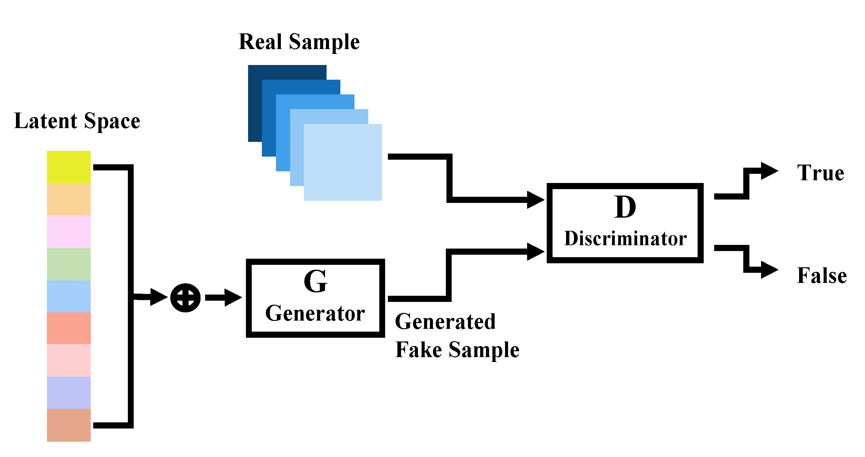
20] and generative adversarial network (GAN) [21] are the representative methods of generative models.
Liu [22] and Su [23] used VAEs to ensure the diversity of the generated data that were sampled from the latent space. However, the generated HSI virtual samples are often ambiguous, which cannot guarantee similarities with the real HSI data. Therefore, GANs have also been applied for HSI generation to improve the quality of generated virtual data. GANs strengthen the ability of discriminators to distinguish the true data sources from the false by introducing “Nash equilibrium” [24,25,26,27,28,29]. For example, Zhan [30] designed a 1-D GAN (HSGAN) to generate the virtual HSI pixels similar to the real ones, thus improving the performance of the classifier. Feng [31] devised two generators to generate 2D-spatial and 1D-spectral information respectively. Zhu [32] exploited 1D-GAN and 3D-GAN architectures to enhance the classification performance. However, GANs are prone to mode collapse, resulting in poor generalization ability of HSI classification.
To overcome the limitations of VAEs and GANs, VAE-GAN jointed framework has been proposed for HSIC. Wang proposed a conditional variational autoencoder with an adversarial training process for HSIC (CVA 2 E) [33]. In this work, GAN was spliced with VAE to realize high-quality restoration of the samples and achieve diversity. Tao et al. [34] proposed the semi-supervised variational generative adversarial networks with a collaborative relationship between the generation network and the classification network to produce meaningful samples that contribute to the final classification. To sum up, in VAE-GAN frameworks, VAE focuses on encoding the latent space, providing creativity of generated samples, while GAN concentrates on replicating the data, contributing to the high quality of virtual samples.
Spectral and spatial are two typical characteristics of HSI, both of which must be taken into account for HSIC. Nevertheless, the distributions of spectral and spatial features are not identical. Therefore, it is difficult to cope with such a complex situation for a single encoder in VAEs. Meanwhile, most of the existing generative methods use spectral and spatial features respectively for HSIC, which affects the generative model to generate realistic virtual samples. In fact, the spectral and spatial features are closely correlated, which cannot be treated separately. Interaction between spectral and spatial information should be established to refine the generated virtual samples for better classification performance.
In this paper, a variational generative adversarial network with crossed spatial and spectral interactions (CSSVGAN) was proposed for HSIC, which consists of a dual-branch variational Encoder, a crossed interactive Generator, and a Discriminator stuck together with a classifier. The dual-branch variational Encoder maps spectral and spatial information to different latent spaces. The crossed interactive Generator reconstructs the spatial and spectral samples from the latent spectral and spatial distribution in a crossed manner. Notably, the intersectional generation process promotes the consistency of learned spatial and spectral features and simulates the highly correlated spatial and spectral characteristics of true HSI. The Discriminator receives the samples from both generator and original training data to distinguish the authenticity of the data. To sum up, the variational Encoder ensures diversity, and the Generator guarantees authenticity. The two components place higher demands on the Discriminator to achieve better classification performance.
Compared with the existing literature, this paper is expected to make the following contributions:
  • The dual-branch variational Encoder in the jointed VAE-GAN framework is developed to map spectral and spatial information into different latent spaces, provides discriminative spectral and spatial features, and ensures the diversity of generated virtual samples.
  • The crossed interactive Generator is proposed to improve the quality of generated virtual samples, which exploits the consistency of learned spatial and spectral features to imitate the highly correlated spatial and spectral characteristics of HSI.
  • The variational generative adversarial network with crossed spatial and spectral interactions is proposed for HSIC, where the diversity and authenticity of generated samples are enhanced simultaneously.
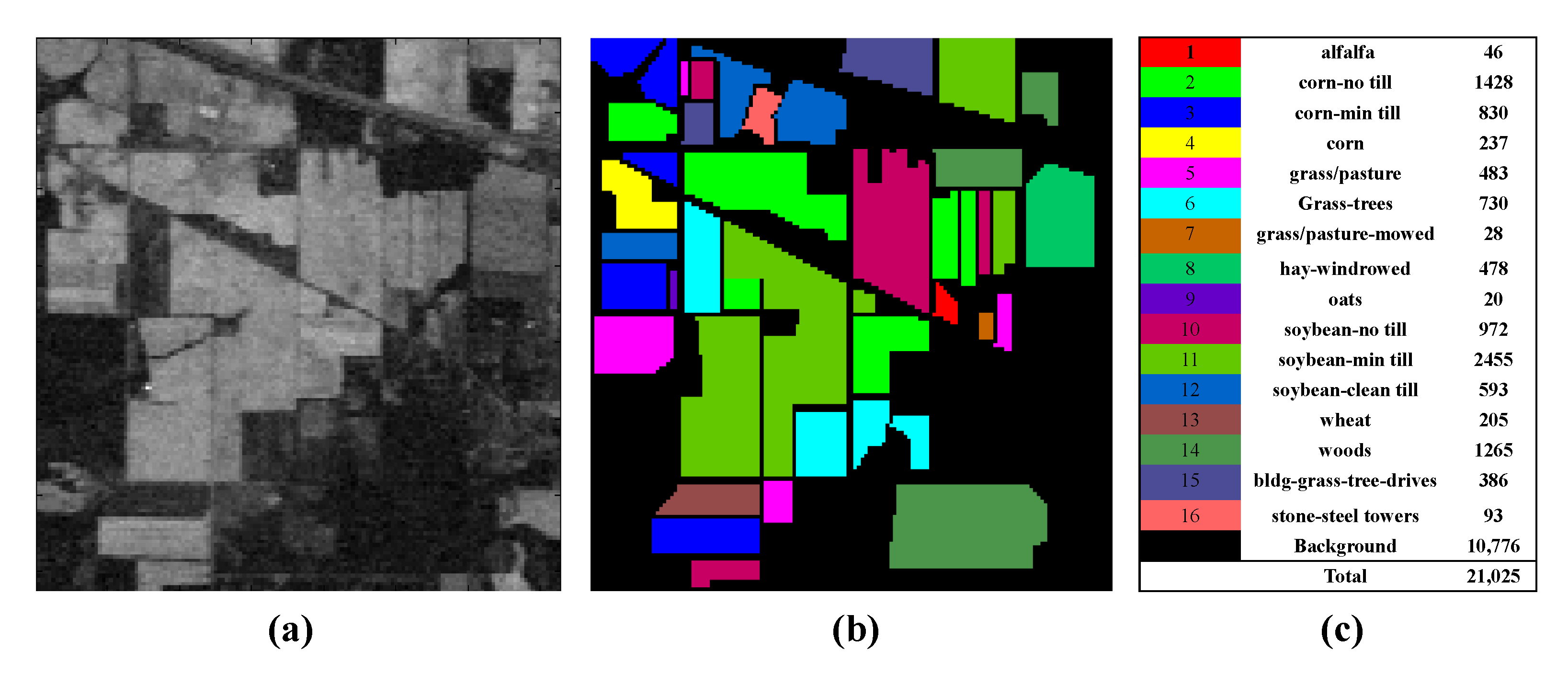
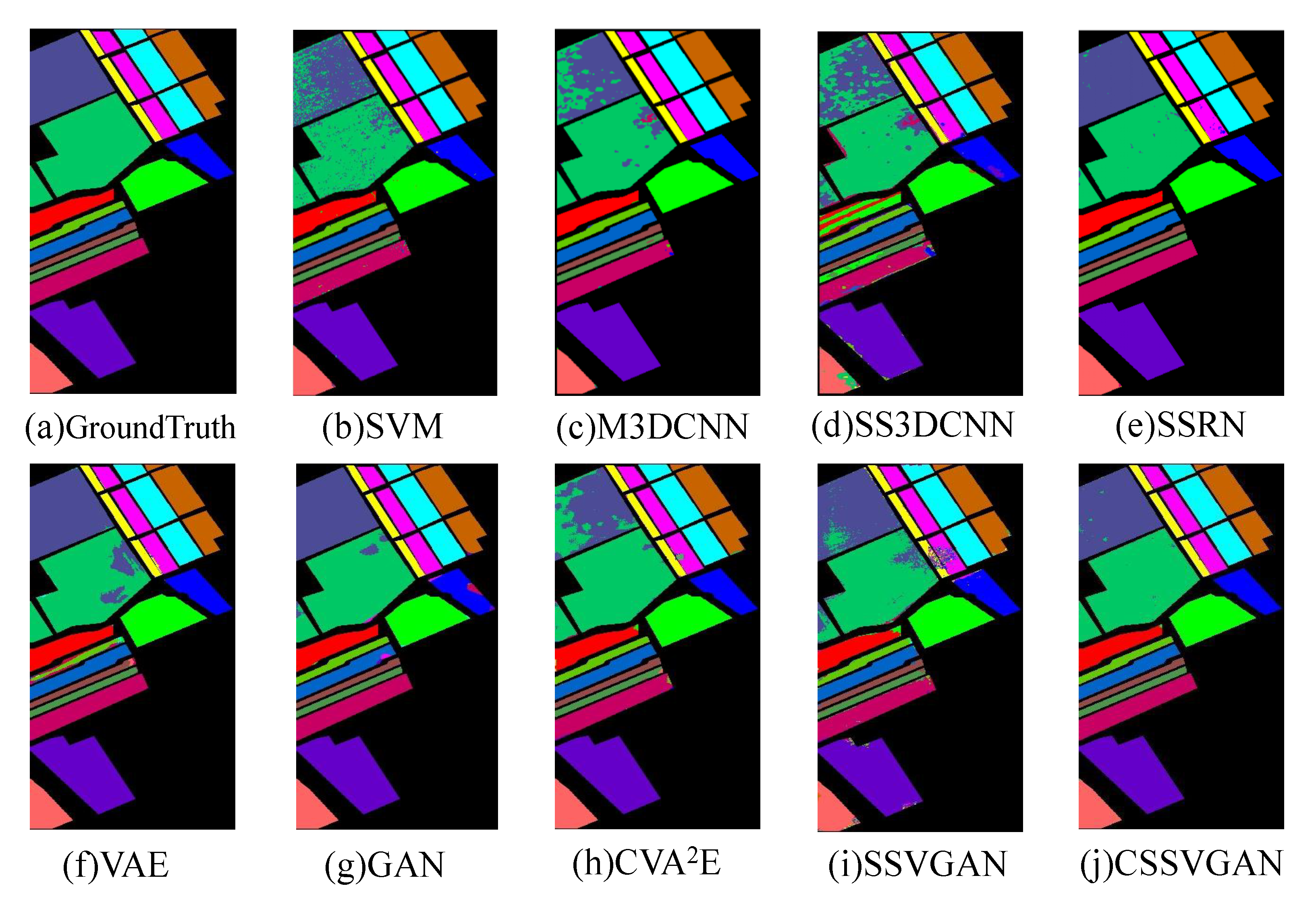
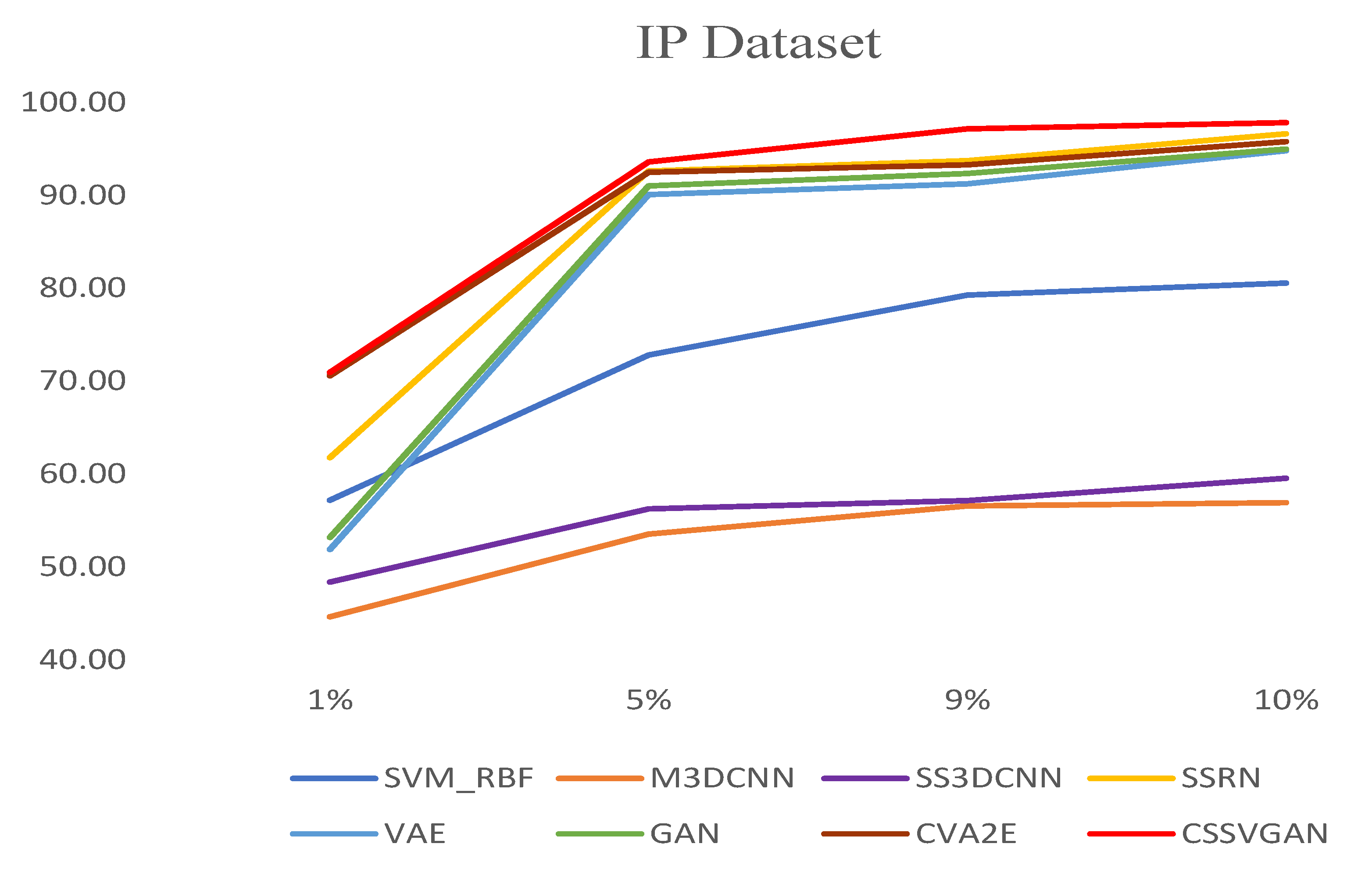
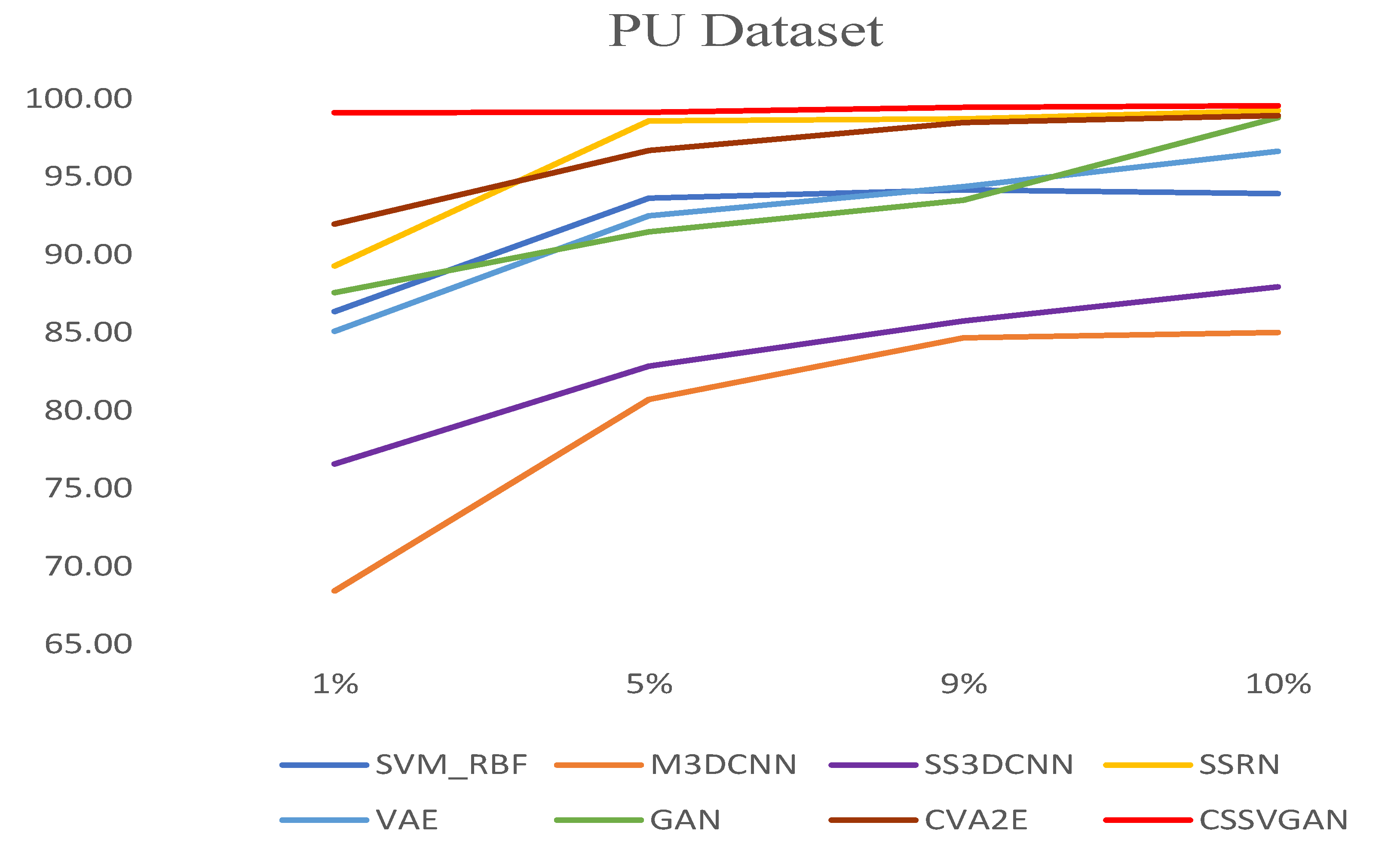
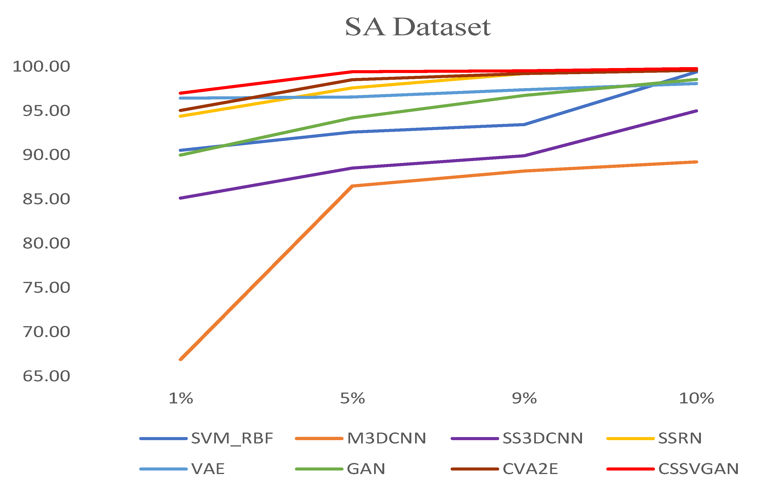
  • Experimental results on the three public datasets demonstrate that the proposed CSSVGAN achieves better performance compared with other well-known models.
The remainder of this paper is arranged as follows. Section 2 introduces VAEs and GANs. Section 3 provides the details of the CSSVGAN framework and the crossed interactive module. Section 4 evaluates the performance of the proposed CSSVGAN through comparison with other methods. The results of the experiment are discussed in Section 5 and the conclusion is given in Section 6.

2. Related Work

2.1. Variational Autoencoder

Variational autoencoder is one variant of the standard AE, proposed by Kingma et al. for the first time [35]. The essence of VAE is to construct an exclusive distribution for each sample X and then sample it represented by Z. It brings Kullback–Leibler [36] divergence penalty method into the process of sampling and constrains it. Then the reconstructed data can be translated to generated simulation data through deep training. The above principle gives VAE a significant advantage in processing hyperspectral images with expensive and rare samples. VAE model adopts the posterior distribution method to verify that ρ ( Z | X ) rather than ρ ( Z ) obeys the normal distribution. Then it manages to find the mean μ and variance σ of ρ ( Z | X k ) corresponding to each X k through the training of neural networks (where X k represents the sample of the original data and ρ ( Z | X k ) represents the posterior distribution). Another particularity of VAE is that it makes all ρ ( Z | X ) align with the standard normal distribution N ( 0 , 1 ) . Taking account of the complexity of HSI data, VAE has superiority over AE in terms of noise interference [37]. It can prevent the occurrence of zero noise, increase the diversity of samples, and further ensure the generation ability of the model.
A VAE model is consists of two parts: Encoder M and Decoder N. M is an approximator for the probability function m τ ( z | x ) , and N is to generate the posterior’s approximate value n θ ( x , z ) . τ and θ are the parameters of the deep neural network, aiming to optimize the following objective functions jointly.
V ( P , Q ) = K L ( m τ ( z | x ) p θ ( z | x ) ) + R ( x ) ,
Among them, R is to calculate the reconstruction loss of a given sample x in the VAE model. The framework of VAE is described in Figure 1, where e i represents the sample of standard normal distribution, corresponding with X k one to one.

2.2. Generative Adversarial Network

Generative adversarial network is put forward by Goodfellow et al. [24], which trains the generation model with a minimax game based on the game theory. The GAN has gained remarkable results in representing the distribution of latent variables for its special structure, which has attracted more attention from the field of visual image processing. A GAN model includes two subnets: the generator G, denoted as G ( z ; θ g ) and the discriminator D, denoted as G ( x ; θ d ) , and θ g and θ d are defined as parameters of the deep neural networks. G shows a prominent capacity in learning the mapping of latent variables and synthesizing new similar data from mapping represented by G ( z ) . The function of D is to take the original HSI or the fake image generated by G as input and then distinguish its authenticity. The architecture of GAN is shown in Figure 2.
After the game training, G and D would maximize log-likelihood respectively and achieve the best generation effect by competing with each other. The expression of the above process is as follows:
m i n G m a x G V ( G , D ) = E x P ( x ) [ log D ( x ) ] + E x P g ( z ) [ log ( 1 D ( G ( z ) ) ) ] ,
where P ( x ) represents the real data distribution and P g ( z ) means the samples’ distribution generated by G. The game would reach a global equilibrium situation between the two players when P ( x ) equaling to P g ( z ) happened. In this case, the best performance of D ( x ) can be expressed as:
D ( x ) m a x = P ( x ) + P g ( x ) ,
However, the over-confidence of D would cause inaccurate results of GAN’s identification and make the generated data far away from the original HSI. To tackle the problem, endeavors have been made to improve the accuracy of HSIC by modifying the loss, such as WGAN [38], LSGAN [39], CycleGAN [40] and so on. Salimans [41] raised a deep convolutional generative adversarial network (DCGAN) to enhance the stability of the training and improve the quality of the results. Subsequently, Alec et al. [42] proposed a one-side label smoothing idea named improved DCGAN, which multiplied the positive sample label by alpha and the negative sample label by beta, that is, the coefficients of positive and negative samples in the objective function of D were no longer from 0 to 1, but from α to β . ( β in the real application could be set to 0.9). It aimed to solve the problems described as follows:
D ( x ) = α P ( x ) + β P g ( x ) P ( x ) + P g ( x ) ,
In this instance, GAN can reduce the disadvantage of overconfidence and make the generated samples more authentic.

3. Methodology

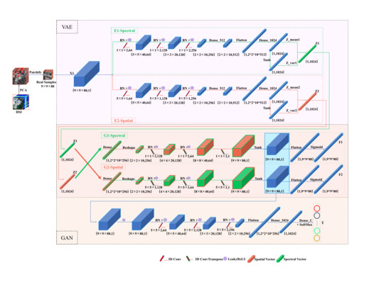
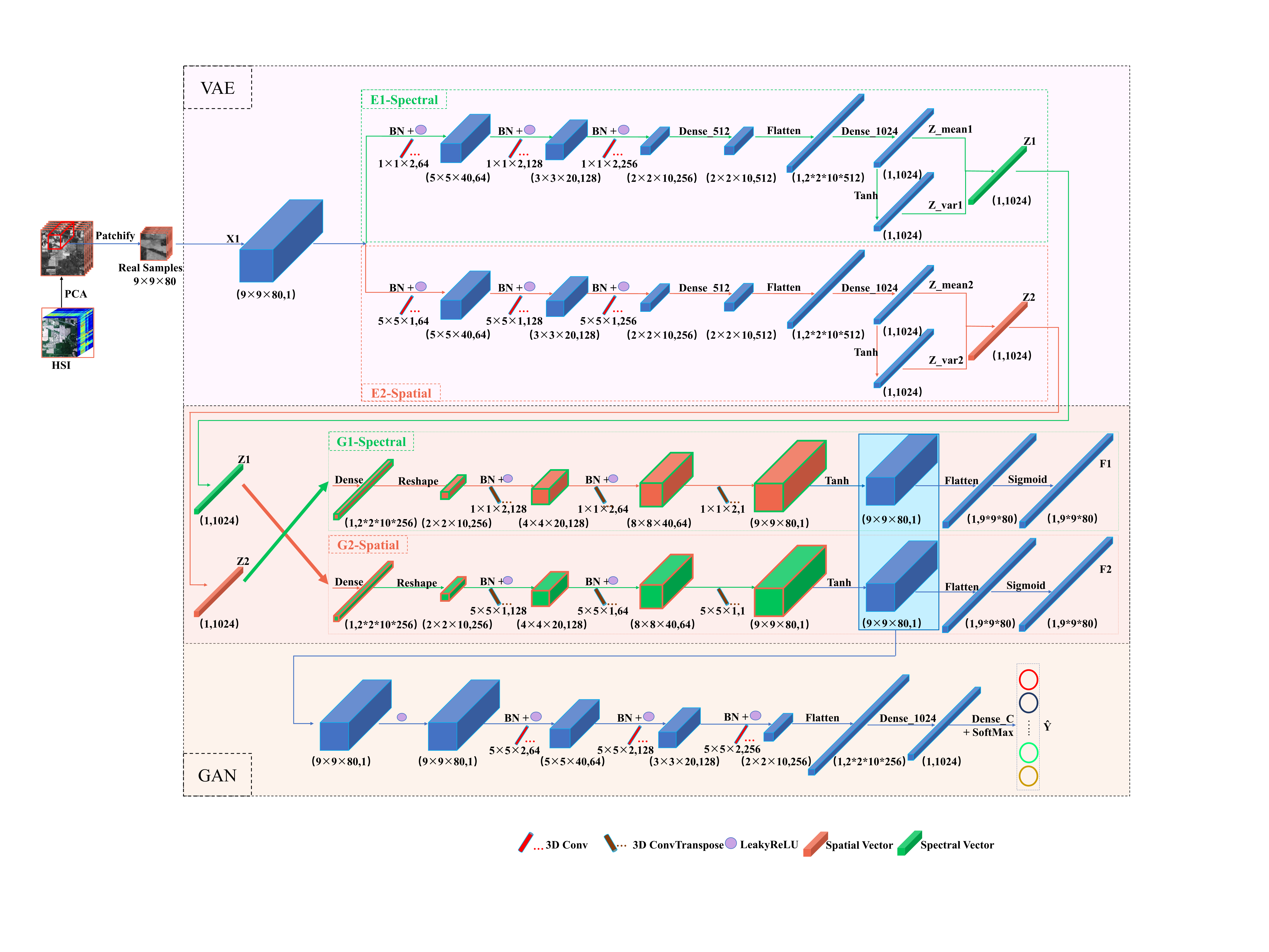
3.1. The Overall Framework of CSSVGAN

The overall framework of CSSVGAN is shown in Figure 3. In the process of data preprocessing, assuming that HSI cuboid X contains n pixels; the spectral band of each pixel is defined as p x ; and X can be expressed as X ϵ R n p x . Then HSI is divided into several patch cubes of the same size. The labeled pixels are marked as X 1 = x i 1 ϵ R ( s s p x n 1 ) , and the unlabeled pixels are marked as X 2 = x i 2 ϵ R ( s s p x n 2 ) . Among them, s, n 1 and n 2 stand for the adjacent spatial sizes of HSI cuboids, the number of labeled samples and the number of unlabeled samples respectively, and n equals to n 1 plus n 2 .
It is noteworthy that HSI classification is developed at the pixel level. Therefore, in this paper, the CSSVGAN framework uses a cube composed of patches of size 9 × 9 × p x as the inputs of the Encoder, where p denotes the spectral bands of each pixel. Then a tensor represents the variables and outputs of each layer. Firstly, the spectral latent variable Z 1 and the spatial latent variable Z 2 are obtained by taking the above X 1 as input into the dual-branch variational Encoder. Secondly, these two inputs are taken to the crossed interactive Generator module to obtain the virtual data F 1 and F 2 . Finally, the data are mixed with X 1 into the Discriminator for adversarial training to get the predicted classification results Y ^ = y ^ i by the classifier.

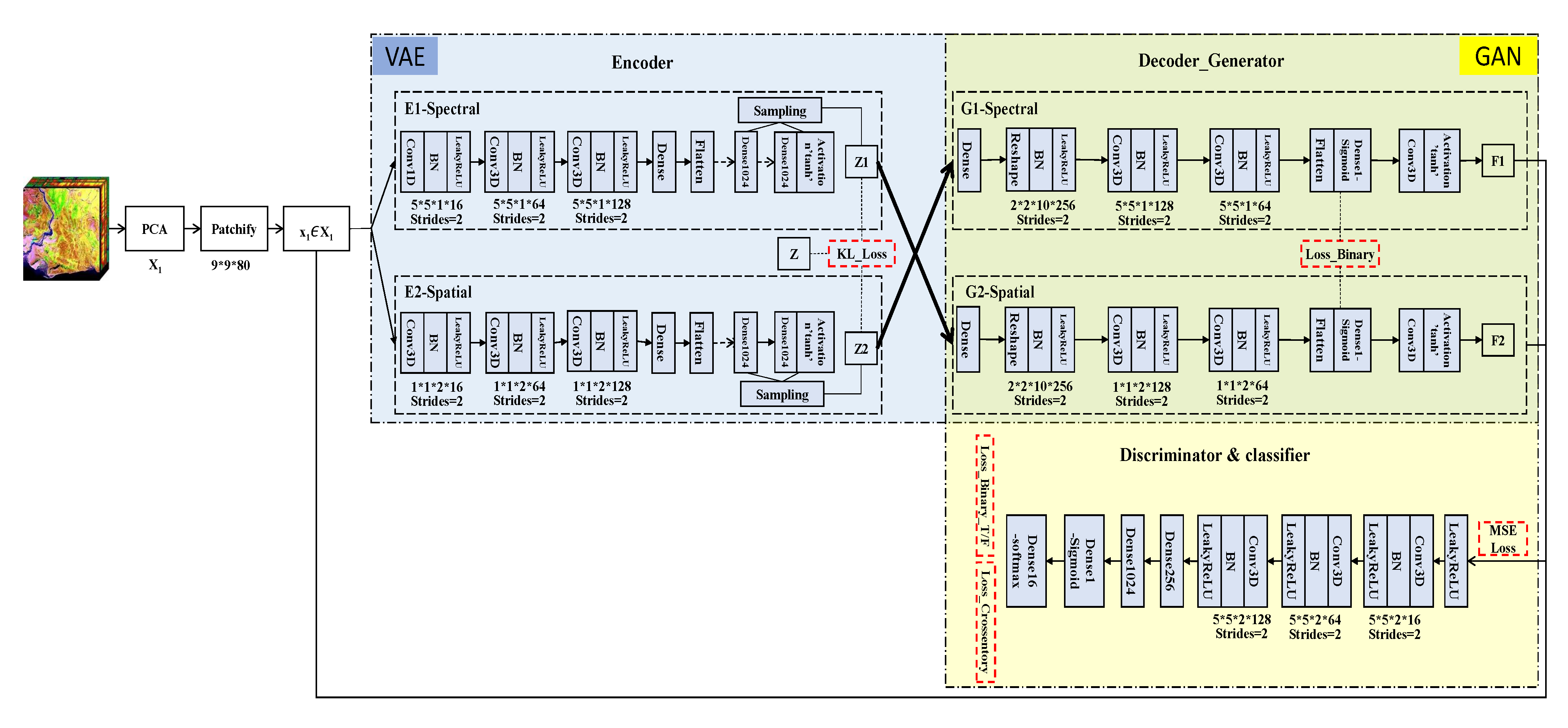
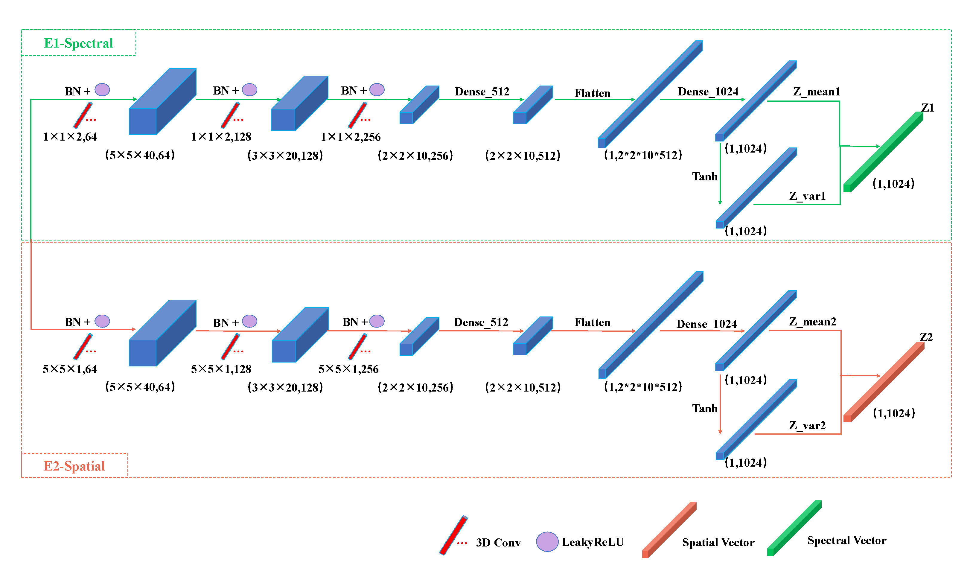
3.2. The Dual-Branch Variational Encoder in CSSVGAN

In the CSSVGAN model mentioned above, the Encoder (Figure 4) is composed of a dual-branch spatial feature extraction E 1 and a spectral feature extraction E 1 to generate more diverse samples. In the E 1 module, the size of the 3D convolution kernel is ( 1 × 1 × 2 ) , the stride is ( 2 , 2 , 2 ) and the spectral features are marked as Z 1 . The implementation details are described in Table 1. Identically, in the E 2 module, the 3D convolution kernels, the strides and the spatial features are presented by ( 5 × 5 × 1 ) , ( 2 , 2 , 2 ) and Z 2 respectively, as described in Table 2.
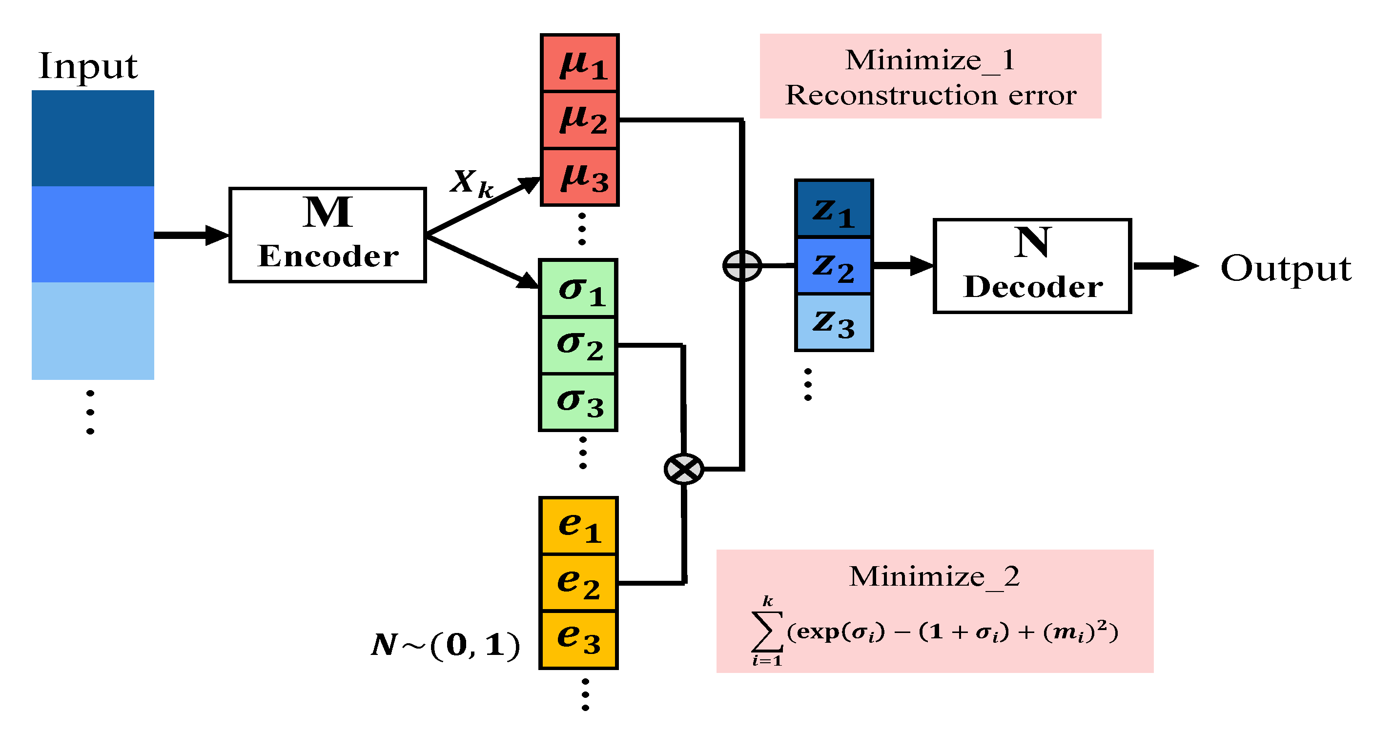
Meanwhile, to ensure the consistent distribution of samples and original data, KL divergence principle is utilized to constrain Z 1 and Z 2 separately. Assuming that the mean and variance of Z i are expressed as Z m e a n i and Z v a r i ( i = 1 , 2 ) , the loss function in the training process is as follows:
L i ( θ , φ ) = K L ( q φ ( z i | x ) p θ ( z i | x ) ) ,
where p ( z i | x ) is the posterior distribution of potential eigenvectors in the Encoder module, and its calculation is based on the Bayesian formula as shown below. But when the dimension of Z is too high, the calculation of P ( x ) is not feasible. At this time, a known distribution q ( z i | x ) is required to approximate p ( z i | x ) , which is given by KL divergence. By minimizing KL divergence, the approximate p ( z i | x ) can be obtained. θ and φ represent the parameters of distribution function p and q separately.
L i ( θ , φ ) = E q φ ( z i , x ) [ log p θ ( x , z i ) q φ ( z i , x ) ] E q ( x ) [ log q ( x ) ] ,
Formula (6) in the back is provided with a constant term l o g N , the entropy of empirical distribution q ( x ) . The advantage of it is that the optimization objective function is more explicit, that is, when p θ ( z i , x ) is equal to q φ ( z i , x ) , KL dispersion can be minimized.

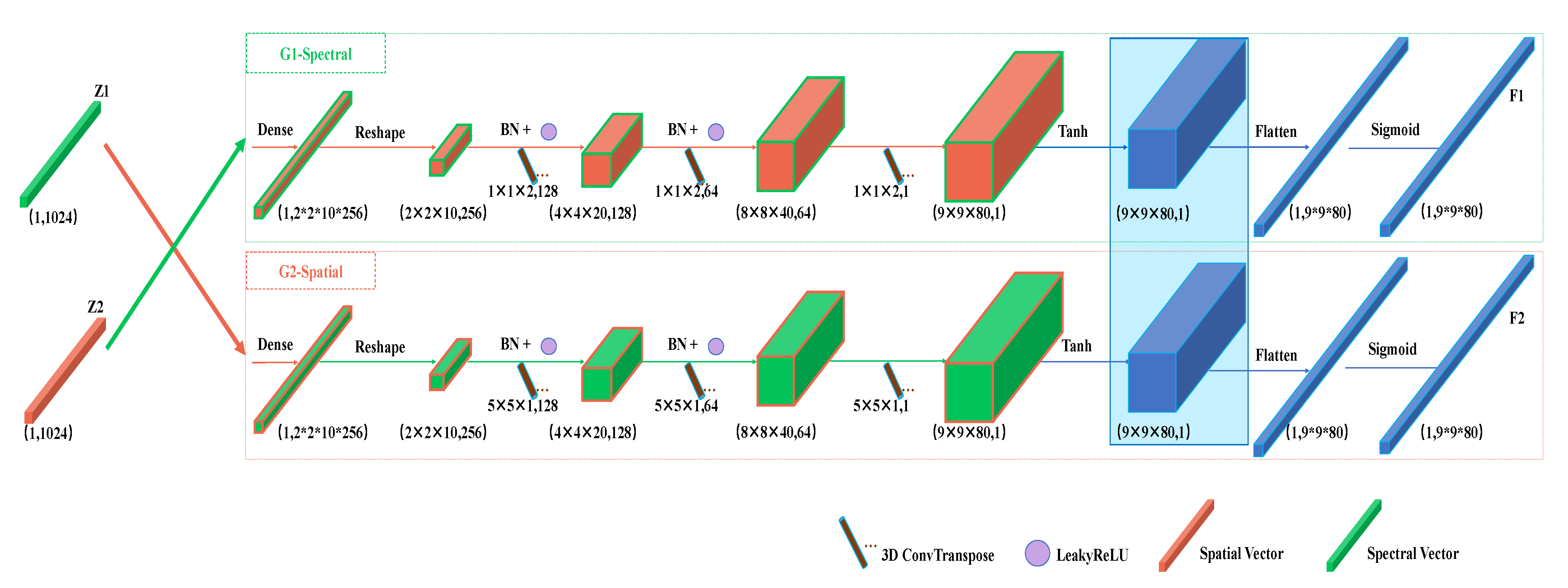
3.3. The Crossed Interactive Generator in CSSVGAN

In CSSVGAN, the crossed interactive Generator module plays a role in data restoration of VAE and data expansion of GAN, which includes the spectral Generator G 1 and the spatial Generator G 2 in the crossed manner. G 1 accepts the spatial latent variables Z 2 to generate spectral virtual data F 1 , and G 2 accepts the spectral latent variables Z 1 to generate spatial virtual data F 2 .
As shown in Figure 5, the 3D convolution of spectral Generator G 1 is ( 1 × 1 × 2 ) that uses ( 2 , 2 , 2 ) strides to convert the spatial latent variables Z 2 to the generated samples. Similarly, the spatial Generator G 2 with ( 5 × 5 × 1 ) convolution uses ( 2 , 2 , 2 ) strides to transform the spectral latent variables Z 1 into generated samples. Therefore, the correlation between spectral and spatial features in HSI can be fully considered to further improve the quality and authenticity of the generated samples. The implementation details of G 1 and G 2 are described in Table 3 and Table 4.
Because the mechanism of GAN is that the Generator and Discriminator are against each other before reaching the Nash equilibrium, the Generator has two target functions, as shown below.
M S E L o s s _ i = 1 n ( y i j y ¯ i j ) 2 ,
where n is the number of samples, i = 1 , 2 , y j means the label of virtual samples, and y ¯ j represents the label of the original data corresponding to y j . The above formula makes the virtual samples generated by crossed interactive Generator as similar as possible to the original data.
B i n a r y L o s s _ i = 1 N j = 1 N y i j · log ( p ( y i j ) ) + ( 1 y i j · ( 1 p ( y i j ) ) ) ,
B i n a r y L o s s is a logarithmic loss function and can be applied to the binary classification task. Where y is the label (either true or false), and p ( y ) is the probability that N sample points belonging to the real label. Only if y j equals to p ( y i ) , the total loss would be zero.

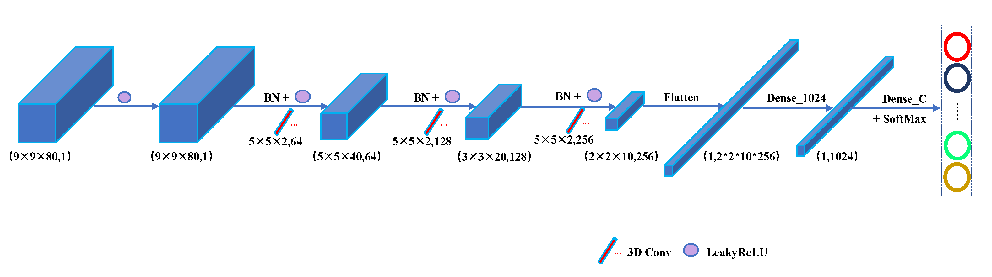
3.4. The Discriminator Stuck with a Classifier in CSSVGAN

As shown in Figure 6, the Discriminator needs to specifically identify the generated data as false and the real HSI data as true. This process can be regarded as a two-category task using one-sided label smoothing: defining the real HSI data as 0.9 and the false as zero. The loss function of it marked with B i n a r y ( L o s s D ) is the same as the Formula (10) enumerated above. Moreover, the classifier is stuck as an interface to the output of Discriminator and the classification results are calculated directly through the SoftMax layer, where C represents the total number of labels in training data. As mentioned above, the Encoder ensures diversity and the Generator guarantees authenticity. All these contributions place higher demands on Discriminator to achieve better classification performance. Thus, the CSSVGAN framework yields a better classification result.
The implementation details of the Discriminator in CSSVGAN are described in Table 5 with the 3D convolution of ( 5 × 5 × 2 ) and strides of ( 2 , 2 , 2 ) . Identifying C categories belongs to a multi-classification assignment. The SoftMax method is taken as the standard for HSIC. As shown below, the CSSVGAN method should allocate the sample x of each class c to the most likely one of the C classes to get the predicted classification results. The specific formula is as follows:
y i = S ( x i ) = e x i j = 1 C e x j ,
Then the category of X can be expressed as the formula below:
c l a s s ( c ) = arg max i ( y i = S ( x i ) ) ,
where S, C, X, Y i signify the SoftMax function, the total number of categories, the input of SoftMax, and the probability that the prediction object belongs to class C, respectively. X i similar with X j is a sample of one certain category. Therefore, the following formula can be used for the loss function of objective constraint.
C L o s s = i = 1 n p ( y i 1 ) · log y i 1 + p ( y i 2 ) · log ( y i 2 ) + · · · + p ( y i c ) · log ( y i c ) ,
where n means the total number of samples, C represents the total number of categories, and y denotes the single label (either true or false) with the same description as above.

3.5. The Total Loss of CSSVGAN

As illustrated in Figure 3, up till now, the final goal of the total loss of the CSSVGAN model can be divided into four parts: two KL divergence constraint losses and a mean-square error loss from the Encoder, two binary losses from the Generator, one binary loss from the Discriminator and one multi-classification loss from the multi classifier. The ensemble formula can be expressed as:
L T o t a l = σ 1 L 1 ( θ , φ ) + σ 2 L 2 ( θ , φ ) + σ 3 M S E L o s s 1 _ 2 E n c o d e r _ L o s s + σ 4 B i n a r y L o s s 1 + σ 5 B i n a r y L o s s 2 G e n e r a t o r _ L o s s + B i n a r y _ L o s s D D i s c r m i n a t o r _ L o s s + C L o s s C l a s s i f i e r _ L o s s ,
where L 1 and L 2 represent the loss between Z 1 or Z 2 and the standard normal distribution respectively in Section 3.2. M S E L o s s 1 and M S E L o s s 2 signify the mean square error of y 1 and y 2 in Section 3.3 separately. M S E L o s s 1 _ 2 calculates the mean square error between y 1 and y 2 . The purpose of B i n a r y L o s s 1 and B i n a r y L o s s 2 is to assume that the virtual data F 1 and F 2 (in Section 3.3) are true with a value of one. B i n a r y L o s s D denotes that the Discriminator identifies F 1 and F 2 as false data with a value of zero. Finally, the C L o s s is the loss of multi classes of the classifier.

4. Experiments

4.1. Dataset Description

In this paper, three representative hyperspectral datasets recognized by the remote sensing community (i.e., Indian Pines, Pavia University and Salinas) are accepted as benchmark datasets. The details of them are as follows:
(1) Indian pines (IP): The first dataset was accepted for HSI classification imaged by Airborne Visible/Infrared Imaging Spectrometer (AVIRIS) in Northwestern Indiana in the USA. It includes 16 categories with a spatial resolution of approximately 20 m per pixel. Samples are shown in Figure 7. The spectral of AVIRIS coverage ranges from 0.4 to 2.5 μ m and includes 200 bands for continuous imaging of ground objects (20 bands are influenced by noise or steam, so only 200 bands are left for research), bring about the total image size of 145 × 145 × 200 . However, since it contains a complex sample distribution, the category samples of training labels were very imbalanced. As some classes have more than 2000 samples while some have less than 30 merely, it is relatively difficult to achieve a high-precision classification of IP HSI.
(2) Pavia University (PU): The second dataset was a part of the hyperspectral image data of the Pavia city in Italy, photographed by the German airborne reflective optics spectral imaging system (Rosis-03) in 2003, containing 9 categories (see Figure 8). The resolution of this spectral imager is 1.3 m, including continuously 115 wavebands in the range of 0.43–0.86 μ m. Among these bands, 12 bands were eliminated due to the influence of noise. Therefore, the images with the remaining 103 spectral bands in size 610 × 340 are normally used.
(3) Salinas (SA): The third dataset recorded the image of Salinas Valley in California, USA, which was also captured by AVIRIS. Unlike the IP dataset, it has a spatial resolution of 3.7 m and consists of 224 bands. However, researchers generally utilize the image of 204 bands after excluding 20 bands affected by water reflection. Thus, the size of the Salinas is 512 × 217 , and Figure 9 depicts the color composite of the image as well as the ground truth map.

4.2. Evaluation Measures

In the experiments, the available data of these datasets were randomly divided into two parts, a small part for training and the rest for testing. Whether the training samples or the testing samples were arranged according to the pixels, whose size was in 1 × p x ( p x is selected as 80 in this paper). Each pixel can be treated as a feature of a certain class, corresponding to a unique label and classified by the classifier stuck to the Discriminator. Table 6, Table 7 and Table 8 list the sample numbers for the training and testing of three datasets.
Taking the phenomenon of “foreign matter of the same spectrum in surface cover” [15,43] into consideration, the average accuracy was reported to evaluate the experiment results quantitatively. Meanwhile, the proposed method was contrasted with the comparative method by three famous indexes, i.e., overall accuracy (OA), average accuracy (AA) and kappa coefficient (KA) [44], which can be denoted as below:
OA = s u m ( d i a g ( M ) ) / s u m ( M ) ,
AA = m e a n ( ( d i a g ( M ) . / ( s u m ( M , 2 ) ) ,
Kappa = OA s u m ( M , 1 ) × s u m ( M , 2 ) / ( s u m ( M ) ) 2 1 s u m ( M , 2 ) / ( s u m ( M ) ) 2 ,
where m represents the number of land cover categories and M ϵ R ( m × n ) symbolizes the confusion matrix of the classification results. Then, d i a g ( M ) ϵ R m × 1 comes to be a vector of diagonal elements in M, s u m ( ) ϵ R 1 proves to be the sum of all elements of matrices, where ( , 1 ) means each column and ( , 2 ) means each row. Finally, the m e a n ( ) ϵ R 1 describes the mean value of all elements along with the . / , which implies the element-wise division.

4.3. Experimental Setting

In this section, for the sake of verifying the effectiveness of CSSVGAN, several classical hyperspectral classification methods such as SVM [45], Mulit-3DCNN [46], SS3DCNN [47], SSRN [15] and certain deep generative algorithms like VAE, GAN and some jointed VAE-GAN models like the CVA 2 E [33] and the semisupervised variational generative adversarial networks (SSVGAN) [34] were used for comparison.
To ensure the fairness of the comparative experiments, the best hyperparameter settings were adopted for each method based on their papers. All experiments were executed on the NVIDIA GeForce GTX 2070 SUPER GPU with a memory of 32 GB. Moreover, Adam [48] was used as the optimizer with an initial learning rate of 1 × 10 3 for Generator and 1 × 10 4 for Discriminator, and the training epoch was set to 200.

4.4. Experiments Results

All experiments in this paper were randomly selected train samples from the labeled pixels, and the accuracies of three datasets were reported to two decimal places in this chapter.

4.4.1. Experiments on the IP Dataset

The experimental test on IP Dataset was performed to evaluate the proposed CSSVGAN model quantitatively with other methods for HSIC. For the labeled samples, 5% of each class was randomly selected for training. The quantitative evaluation of various methods is shown in Table 9, which describes the classification accuracy of different categories in detail, as well as the indicators including OA, AA and kappa for different methods. The best value is marked in dark gray.
First of all, although SVM achieves good exactitude, there is still a certain gap from the exact classification because of the IP dataset containing high texture spatial information, which leads to bad performance. Secondly, some conventional deep learning methods (such as M3DCNN, SS3DCNN) does not perform well in some categories due to the limitation of the number of training samples. Thirdly, the algorithms with jointed spectral-spatial feature extraction (like SSRN, etc.) show a better performance, which indicate a necessity to combine spectral information and spatial information for HSIC. Moreover, it is obvious that the generated virtual samples by VAE tend to be fuzzy and cannot guarantee similarities with the real data. While GAN lacks sampling constraints, leading to the low quality of the generated samples. Contrasted with these two deep generative models, CSSVGAN overcomes their shortcomings. Finally, compared with CVA 2 E and SSVGAN, the two latest jointed models published in IEEE, CSSVGAN uses dual-branch feature extractions and crossed interactive method, which proves that these manners are more suitable for HSIC works. It can increase the diversity of samples and promote the generated data more similar to the original.
Among these comparative methods, CSSVGAN acquires the best accuracy in OA, AA and kappa, which improves by 2.57%, 1.24% and 3.81% respectively, at least. In addition, although all the methods have different degrees of misclassification, CSSVGAN achieves perfect accuracy in “Oats” “Wheat” and so on. The classification visualizations on the Indian Pines of comparative experiments are shown in Figure 10.
From Figure 10, it can be seen that CSSVGAN reduces the noisy scattering points and effectively improves the regional uniformity. That is because CSSVGAN can generate more realistic images from diverse samples.

4.4.2. Experiments on the PU Dataset

Differ from the IP dataset experiments, 1% labeled samples were selected for training and the rest for testing. Table 10 shows the quantitative evaluation of each class in comparative experiments. The best accurate value is marked in dark gray to emphasize, and the classification visualizations on the Pavia university are shown in Figure 11.
Table 10 shows that, as a non-deep learning algorithm, SVM has been able to improve the classification result to 86.36%, which is wonderful to some extent. VAE shows good performance in the training of the “Painted metal sheets” class but low accuracy in the “Self-blocking bricks” class, which leads to the “fuzzy” phenomenon of a single VAE network in the training of individual classes. SSRN achieves a completely correct classification in “shadows,” but it lost to the CSSVGAN overall. In the index of OA results, CSSVGAN improved 12.75%, 30.68%, 22.52%, 9.83%, 14.03%, 11.53%, 7.14% and 6.18% respectively and in the index of Kappa results, CSSVGAN improved 17.07%, 42.23%, 30.03%, 13.62%, 19.25%, 15.16%, 13.19% and 8.3% respectively compared with the other eight algorithms.
In Figure 11, the proposed CSSVGAN has better boundary integrity and better classification accuracy in most of the classes because the Encoder can ensure the diversity of samples, the Generator can promote the authenticity of the generated virtual data, and the Discriminator can adjust the overall framework to obtain the optimal results.

4.4.3. Experiments on the SA Dataset

The experimental setting on the Salinas dataset is the same as PU. Table 11 shows the quantitative evaluation of each class in various methods with dark gray to emphasize the best results. The classification visualization of the comparative experiments on Salinas is shown in Figure 12.
Table 11 shows that in the index of OA, AA and Kappa, CSSVGAN improved 0.57%, 1.27% and 0.62% at least compared with others. Moreover, it has a better performance in the “brocoli-green-weeds-1” and “stubble” class with a test accuracy of 100%. For the precisions of other classes, although SSRN, VAE or SSRN prevails, CSSVGAN is almost equal to them. It can be seen that CSSVGAN has smoother edges and the minimum misclassification in Figure 12, which further proves that the proposed CSSVGAN can generate more realistic virtual data according to the diversity of extracted features of samples.

5. Discussions

5.1. The Ablation Experiment in CSSVGAN

Taking IP, PU and SA datasets as examples, the frameworks of ablation experiments are shown in Figure 13, including NSSNCSG, SSNCSG and SSNCDG.
As shown in Table 12, compared with NSSNCSG, the OA of CSSVGAN on IP, PU and SA datasets increased by 1.02%, 6.90% and 4.63%, respectively.
It shows that the effect of using dual-branch special-spatial feature extraction is better than not using it because the distributions of spectral and spatial features are not identical, and a single Encoder cannot handle this complex situation. Consequently, using the dual-branch variational Encoder can increase the diversity of samples. Under the constraint of KL divergence, the distribution of latent variables is more consistent with the distribution of real data.
Contrasted with SSNCSG, the OA index on IP, PU and SA datasets increase by 0.99%, 1.07% and 0.39% respectively, which means that the result of utilizing the crossed interactive method is more effective, and further influences that the crossed interactive double Generator can fully learn the spectral and spatial information and generate spatial and spectral virtual samples in higher qualities.
Finally, a comparison is made between SSNCDG and CSSVGAN, where the latter can better improve the authenticity of virtual samples by crossed manner. All these contributions of both the Encoder and the Generator put forward higher requirements to the Discriminator, optimizing Discriminator’s ability to identify the true or false data and further achieve the final classification results more accurately.

5.2. Sensitivity to the Proportion of Training Samples

To verify the effectiveness of the proposed CSSVGAN, three datasets were taken as examples. The percentage of training samples was changed for each class from 1% to 9% at 4% intervals and added 10%. Figure 14, Figure 15 and Figure 16 shows the OAs of all the comparative algorithms with various percentages of training samples.
It can be seen that the CSSVGAN has the optimal effect in each proportion of training samples in three datasets because CSSVGAN can learn the extracted features interactively, ensure diverse samples and improve the quality of generated images.

5.3. Investigation of the Proportion of Loss Function

Taking the IP dataset as an example, the proportion σ i ( i = 1 , 2 , 5 ) of loss functions and other super parameters of each module are adjusted to observe their impact on classification accuracy and the results are recorded in Table 13 (the best results are marked in dark gray). Moreover, the learning rate is also an important factor, which will not be repeated here. It can be obtained by experiments that using 1 × 10 3 for Generator and 1 × 10 4 for Discriminator are the best assignments.
Analyzing Table 13 reveals that when σ 1 σ 5 are set as 0.35, 0.35, 0.1, 0.1 and 0.1 respectively, the CSSVGAN model achieves the best performance. Under this condition, the Encoder can acquire the maximum diversity of samples. The Discriminator is able to realize the most accurate classification, and the Generator is capable of generating the images most like the original data. Moreover, the best parameter combination σ 1 σ 5 on the SA dataset is similar to IP, while in the PU dataset, they are set as 0.3, 0.3, 0.1, 0.1 and 0.2.

6. Conclusions

In this paper, variational generative adversarial network with crossed spatial and spectral interactions (CSSVGAN) is proposed for HSIC. It mainly consists of three modules: a dual-branch variational Encoder, a crossed interactive Generator, and a Discriminator stuck with a classifier. From the experiment results of these three datasets, it showed that CSSVGAN can outperform the other methods in the index of OA, AA and Kappa in its abilities because of the dual-branch and the crossed interactive manners. Moreover, using the dual-branch Encoder can ensure the diversity of generated samples by mapping spectral and spatial information into different latent spaces, and utilizing the crossed interactive Generator can imitate the highly correlated spatial and spectral characteristics of HSI by exploiting the consistency of learned spectral and spatial features. All these contributions made the proposed CSSVGAN give the best performance in three datasets. In the future, we will develop towards to realize lightweight generative models and explore the application of the jointed “Transformer and GAN” model for HSIC.

Author Contributions

Conceptualization, Z.L. and X.Z.; methodology, Z.L., X.Z. and L.W.; software, Z.L., X.Z., L.W. and Z.X.; validation, Z.L., F.G. and X.C.; writing—original draft preparation, L.W. and X.Z.; writing—review and editing, Z.L., Z.X. and F.G.; project administration, Z.L. and L.W.; funding acquisition, Z.L. and L.W. All authors read and agreed to the published version of the manuscript.

Funding

This research was funded by the Joint Funds of the General Program of the National Natural Science Foundation of China, Grant Number 62071491, the National Natural Science Foundation of China, Grant Number U1906217, and the Fundamental Research Funds for the Central Universities, Grant No. 19CX05003A-11.

Informed Consent Statement

Informed consent was obtained from all subjects involved in the study.

Data Availability Statement

Publicly available datasets were analyzed in this study, which can be found here: http://www.ehu.eus/ccwintco/index.php?title=Hyperspectral_Remote_Sensing_Scenes, latest accessed on 29 July 2021.

Acknowledgments

The authors are grateful for the positive and constructive comments of editor and reviewers, which have significantly improved this work.

Conflicts of Interest

The authors declare no conflict of interest. The funders had no role in the design of the study; in the collection, analyses, or interpretation of data; in the writing of the manuscript; nor in the decision to publish the results.

References

  1. Chen, P.; Jiao, L.; Liu, F.; Zhao, J.; Zhao, Z. Dimensionality reduction for hyperspectral image classification based on multiview graphs ensemble. J. Appl. Remote Sens. 2016, 10, 030501. [Google Scholar] [CrossRef]
  2. Shi, G.; Luo, F.; Tang, Y.; Li, Y. Dimensionality Reduction of Hyperspectral Image Based on Local Constrained Manifold Structure Collaborative Preserving Embedding. Remote Sens. 2021, 13, 1363. [Google Scholar] [CrossRef]
  3. Atzberger, C. Advances in remote sensing of agriculture: Context description, existing operational monitoring systems and major information needs. Remote Sens. 2013, 5, 949–981. [Google Scholar] [CrossRef] [Green Version]
  4. Sun, Y.; Wang, S.; Liu, Q.; Hang, R.; Liu, G. Hypergraph embedding for spatial-spectral joint feature extraction in hyperspectral images. Remote Sens. 2017, 9, 506. [Google Scholar] [CrossRef] [Green Version]
  5. Abbate, G.; Fiumi, L.; De Lorenzo, C.; Vintila, R. Evaluation of remote sensing data for urban planning. Applicative examples by means of multispectral and hyperspectral data. In Proceedings of the 2003 2nd GRSS/ISPRS Joint Workshop on Remote Sensing and Data Fusion over Urban Areas, Berlin, Germany, 22–23 May 2003; pp. 201–205. [Google Scholar]
  6. Yuen, P.W.; Richardson, M. An introduction to hyperspectral imaging and its application for security, surveillance and target acquisition. Imaging Sci. J. 2010, 58, 241–253. [Google Scholar] [CrossRef]
  7. Tan, K.; Zhang, J.; Du, Q.; Wang, X. GPU parallel implementation of support vector machines for hyperspectral image classification. IEEE J. Sel. Top. Appl. Earth Obs. Remote Sens. 2015, 8, 4647–4656. [Google Scholar] [CrossRef]
  8. Li, J.; Bioucas-Dias, J.M.; Plaza, A. Semisupervised hyperspectral image classification using soft sparse multinomial logistic regression. IEEE Geosci. Remote Sens. Lett. 2012, 10, 318–322. [Google Scholar]
  9. Tan, K.; Hu, J.; Li, J.; Du, P. A novel semi-supervised hyperspectral image classification approach based on spatial neighborhood information and classifier combination. ISPRS J. Photogramm. Remote Sens. 2015, 105, 19–29. [Google Scholar] [CrossRef]
  10. Gao, Q.; Lim, S.; Jia, X. Hyperspectral image classification using convolutional neural networks and multiple feature learning. Remote Sens. 2018, 10, 299. [Google Scholar] [CrossRef] [Green Version]
  11. Chen, Y.; Jiang, H.; Li, C.; Jia, X.; Ghamisi, P. Deep feature extraction and classification of hyperspectral images based on convolutional neural networks. IEEE Trans. Geosci. Remote Sens. 2016, 54, 6232–6251. [Google Scholar] [CrossRef] [Green Version]
  12. Zhang, B.; Zhao, L.; Zhang, X. Three-dimensional convolutional neural network model for tree species classification using airborne hyperspectral images. Remote Sens. Environ. 2020, 247, 111938. [Google Scholar] [CrossRef]
  13. Chen, Y.C.; Lei, T.C.; Yao, S.; Wang, H.P. PM2. 5 Prediction Model Based on Combinational Hammerstein Recurrent Neural Networks. Mathematics 2020, 8, 2178. [Google Scholar] [CrossRef]
  14. Nezami, S.; Khoramshahi, E.; Nevalainen, O.; Pölönen, I.; Honkavaara, E. Tree species classification of drone hyperspectral and rgb imagery with deep learning convolutional neural networks. Remote Sens. 2020, 12, 1070. [Google Scholar] [CrossRef] [Green Version]
  15. Zhong, Z.; Li, J.; Luo, Z.; Chapman, M. Spectral–spatial residual network for hyperspectral image classification: A 3-D deep learning framework. IEEE Trans. Geosci. Remote Sens. 2017, 56, 847–858. [Google Scholar] [CrossRef]
  16. Xu, Y.; Zhang, L.; Du, B.; Zhang, F. Spectral–spatial unified networks for hyperspectral image classification. IEEE Trans. Geosci. Remote Sens. 2018, 56, 5893–5909. [Google Scholar] [CrossRef]
  17. Liu, G.; Gao, L.; Qi, L. Hyperspectral Image Classification via Multieatureased Correlation Adaptive Representation. Remote Sens. 2021, 13, 1253. [Google Scholar] [CrossRef]
  18. Zhao, W.; Du, S. Spectral–spatial feature extraction for hyperspectral image classification: A dimension reduction and deep learning approach. IEEE Trans. Geosci. Remote Sens. 2016, 54, 4544–4554. [Google Scholar] [CrossRef]
  19. Roy, S.K.; Krishna, G.; Dubey, S.R.; Chaudhuri, B.B. HybridSN: Exploring 3-D–2-D CNN feature hierarchy for hyperspectral image classification. IEEE Geosci. Remote Sens. Lett. 2019, 17, 277–281. [Google Scholar] [CrossRef] [Green Version]
  20. Belwalkar, A.; Nath, A.; Dikshit, O. Spectral-Spatial Classification of Hyperspectral Remote Sensing Images Using Variational Autoencoder and Convolution Neural Network. In Proceedings of the International Archives of the Photogrammetry, Remote Sensing and Spatial Information Sciences, Dehradun, India, 20–23 November 2018. [Google Scholar]
  21. Goodfellow, I.; Pouget-Abadie, J.; Mirza, M.; Xu, B.; Warde-Farley, D.; Ozair, S.; Courville, A.; Bengio, Y. Generative adversarial nets. arXiv 2014, arXiv:1406.2661v1. [Google Scholar]
  22. Liu, X.; Gherbi, A.; Wei, Z.; Li, W.; Cheriet, M. Multispectral image reconstruction from color images using enhanced variational autoencoder and generative adversarial network. IEEE Access 2020, 9, 1666–1679. [Google Scholar] [CrossRef]
  23. Su, Y.; Li, J.; Plaza, A.; Marinoni, A.; Gamba, P.; Chakravortty, S. DAEN: Deep autoencoder networks for hyperspectral unmixing. IEEE Trans. Geosci. Remote Sens. 2019, 57, 4309–4321. [Google Scholar] [CrossRef]
  24. Makhzani, A.; Shlens, J.; Jaitly, N.; Goodfellow, I.; Frey, B. Adversarial autoencoders. arXiv 2015, arXiv:1511.05644. [Google Scholar]
  25. Bao, J.; Chen, D.; Wen, F.; Li, H.; Hua, G. CVAE-GAN: Fine-grained image generation through asymmetric training. In Proceedings of the IEEE International Conference on Computer Vision, Venice, Italy, 22–29 October 2017; pp. 2745–2754. [Google Scholar]
  26. He, Z.; Liu, H.; Wang, Y.; Hu, J. Generative adversarial networks-based semi-supervised learning for hyperspectral image classification. Remote Sens. 2017, 9, 1042. [Google Scholar] [CrossRef] [Green Version]
  27. Isola, P.; Zhu, J.Y.; Zhou, T.; Efros, A.A. Image-to-image translation with conditional adversarial networks. In Proceedings of the IEEE Conference on Computer Vision and Pattern Recognition, Honolulu, HI, USA, 21–26 July 2017; pp. 1125–1134. [Google Scholar]
  28. Chen, X.; Duan, Y.; Houthooft, R.; Schulman, J.; Sutskever, I.; Abbeel, P. Infogan: Interpretable representation learning by information maximizing generative adversarial nets. In Proceedings of the 30th International Conference on Neural Information Processing Systems, Kyoto, Japan, 16–21 October 2016; pp. 2180–2188. [Google Scholar]
  29. Feng, J.; Feng, X.; Chen, J.; Cao, X.; Zhang, X.; Jiao, L.; Yu, T. Generative adversarial networks based on collaborative learning and attention mechanism for hyperspectral image classification. Remote Sens. 2020, 12, 1149. [Google Scholar] [CrossRef] [Green Version]
  30. Zhan, Y.; Hu, D.; Wang, Y.; Yu, X. Semisupervised hyperspectral image classification based on generative adversarial networks. IEEE Geosci. Remote Sens. Lett. 2017, 15, 212–216. [Google Scholar] [CrossRef]
  31. Feng, J.; Yu, H.; Wang, L.; Cao, X.; Zhang, X.; Jiao, L. Classification of hyperspectral images based on multiclass spatial–spectral generative adversarial networks. IEEE Trans. Geosci. Remote Sens. 2019, 57, 5329–5343. [Google Scholar] [CrossRef]
  32. Zhu, L.; Chen, Y.; Ghamisi, P.; Benediktsson, J.A. Generative adversarial networks for hyperspectral image classification. IEEE Trans. Geosci. Remote Sens. 2018, 56, 5046–5063. [Google Scholar] [CrossRef]
  33. Wang, X.; Tan, K.; Du, Q.; Chen, Y.; Du, P. CVA2E: A conditional variational autoencoder with an adversarial training process for hyperspectral imagery classification. IEEE Trans. Geosci. Remote Sens. 2020, 58, 5676–5692. [Google Scholar] [CrossRef]
  34. Wang, H.; Tao, C.; Qi, J.; Li, H.; Tang, Y. Semi-supervised variational generative adversarial networks for hyperspectral image classification. In Proceedings of the IGARSS 2019-2019 IEEE International Geoscience and Remote Sensing Symposium, Yokohama, Japan, 28 July–2 August 2019; pp. 9792–9794. [Google Scholar]
  35. Kingma, D.P.; Welling, M. Auto-encoding variational bayes. arXiv 2013, arXiv:1312.6114. [Google Scholar]
  36. Kullback, S.; Leibler, R.A. On information and sufficiency. Ann. Math. Stat. 1951, 22, 79–86. [Google Scholar] [CrossRef]
  37. Wu, C.; Wu, F.; Wu, S.; Yuan, Z.; Liu, J.; Huang, Y. Semi-supervised dimensional sentiment analysis with variational autoencoder. Knowl. Based Syst. 2019, 165, 30–39. [Google Scholar] [CrossRef]
  38. Arjovsky, M.; Chintala, S.; Bottou, L. Wasserstein GAN. arXiv 2017, arXiv:1701.07875. [Google Scholar]
  39. Mao, X.; Li, Q.; Xie, H.; Lau, R.Y.; Wang, Z.; Paul Smolley, S. Least squares generative adversarial networks. In Proceedings of the IEEE International Conference on Computer Vision, Venice, Italy, 22–29 October 2017; pp. 2794–2802. [Google Scholar]
  40. Zhu, J.Y.; Park, T.; Isola, P.; Efros, A.A. Unpaired image-to-image translation using cycle-consistent adversarial networks. In Proceedings of the IEEE International Conference on Computer Vision, Venice, Italy, 22–29 October 2017; pp. 2223–2232. [Google Scholar]
  41. Salimans, T.; Goodfellow, I.; Zaremba, W.; Cheung, V.; Radford, A.; Chen, X. Improved techniques for training gans. Adv. Neural Inf. Process. Syst. 2016, 29, 2234–2242. [Google Scholar]
  42. Radford, A.; Metz, L.; Chintala, S. Unsupervised representation learning with deep convolutional generative adversarial networks. arXiv 2015, arXiv:1511.06434. [Google Scholar]
  43. Imani, M.; Ghassemian, H. An overview on spectral and spatial information fusion for hyperspectral image classification: Current trends and challenges. Inf. Fusion 2020, 59, 59–83. [Google Scholar] [CrossRef]
  44. Sun, H.; Zheng, X.; Lu, X.; Wu, S. Spectral–spatial attention network for hyperspectral image classification. IEEE Trans. Geosci. Remote Sens. 2019, 58, 3232–3245. [Google Scholar] [CrossRef]
  45. Melgani, F.; Bruzzone, L. Classification of hyperspectral remote sensing images with support vector machines. IEEE Trans. Geosci. Remote Sens. 2004, 42, 1778–1790. [Google Scholar] [CrossRef] [Green Version]
  46. He, M.; Li, B.; Chen, H. Multi-scale 3D deep convolutional neural network for hyperspectral image classification. In Proceedings of the 2017 IEEE International Conference on Image Processing (ICIP), Beijing, China, 17–20 September 2017; pp. 3904–3908. [Google Scholar]
  47. Li, Y.; Zhang, H.; Shen, Q. Spectral–spatial classification of hyperspectral imagery with 3D convolutional neural network. Remote Sens. 2017, 9, 67. [Google Scholar] [CrossRef] [Green Version]
  48. Loshchilov, I.; Hutter, F. Sgdr: Stochastic gradient descent with warm restarts. arXiv 2016, arXiv:1608.03983. [Google Scholar]
Figure 1. The framework of VAE.
Remotesensing 13 03131 g001
Figure 2. The architecture of GAN.
Remotesensing 13 03131 g002
Figure 3. The overall framework of the variational generative adversarial network with crossed spatial and spectral interactions (CSSVGAN) for HSIC.
Remotesensing 13 03131 g003
Figure 4. The dual-branch Encoder in CSSVGAN.
Remotesensing 13 03131 g004
Figure 5. The Crossed Interactive Generator in CSSVGAN.
Remotesensing 13 03131 g005
Figure 6. The Discriminator stuck with a classifier in CSSVGAN.
Remotesensing 13 03131 g006
Figure 7. Indian Pines imagery: (a) color composite with RGB, (b) ground truth, and (c) category names with labeled samples.
Remotesensing 13 03131 g007
Figure 8. Pavia University imagery: (a) color composite with RGB, (b) ground truth, and (c) class names with available samples.
Remotesensing 13 03131 g008
Figure 9. Salinas imagery: (a) color composite with RGB, (b) ground truth, and (c) class names with available samples.
Remotesensing 13 03131 g009
Figure 10. Classification maps for the IP dataset with 5% labeled training samples: (a) GroungTruth (b) SVM (c) M3DCNN (d) SS3DCNN (e) SSRN (f) VAE (g) GAN (h) CVA 2 E (i) SSVGAN (j) CSSVGAN.
Remotesensing 13 03131 g010
Figure 11. Classification maps for the PU dataset with 1% labeled training samples: (a) GroungTruth (b) SVM (c) M3DCNN (d) SS3DCNN (e) SSRN (f) VAE (g) GAN (h) CVA 2 E (i) SSVGAN (j) CSSVGAN.
Remotesensing 13 03131 g011
Figure 12. Classification maps for the SA dataset with 1% labeled training samples: (a) GroungTruth (b) SVM (c) M3DCNN (d) SS3DCNN (e) SSRN (f) VAE (g) GAN (h) CVA 2 E (i) SSVGAN (j) CSSVGAN.
Remotesensing 13 03131 g012
Figure 13. The frameworks of ablation experiments: (a) NSSNCSG (b) SSNCSG (c) SSNCDG (d) CSSVGAN.
Remotesensing 13 03131 g013
Figure 14. Sensitivity to the Proportion of Training Samples in IP dataset.
Remotesensing 13 03131 g014
Figure 15. Sensitivity to the Proportion of Training Samples in PU dataset.
Remotesensing 13 03131 g015
Figure 16. Sensitivity to the Proportion of Training Samples in SA dataset.
Remotesensing 13 03131 g016
Table 1. The implementation details of the Spectral feature extraction E 1 .
Input SizeLayer OperationsOutput Size
( 9 × 9 × 80 , 1 ) Conv3D ( 1 × 1 × 2 , 64 ) B N L e a k y R e L U ( 5 × 5 × 40 , 64 )
( 5 × 5 × 40 , 64 ) Conv3D ( 1 × 1 × 2 , 128 ) B N L e a k y R e L U ( 3 × 3 × 20 , 128 )
( 3 × 3 × 20 , 128 ) Conv3D ( 1 × 1 × 2 , 256 ) B N L e a k y R e L U ( 2 × 2 × 10 , 256 )
( 2 × 2 × 10 , 256 ) Dense ( 512 ) B N L e a k y R e L U ( 2 × 2 × 10 , 512 )
( 2 × 2 × 10 , 512 ) Flatten(, 20, 480)
(, 20, 480)Dense ( 1024 ) (, 1024)
( , 1024 ) Dense ( 1024 ) T a n h ( , 1024 )
( , 1024 ) Lambda ( S a m p l i n g ) ( , 1024 )
Table 2. The implementation details of the Spatial feature extraction E 2 .
Input SizeLayer OperationsOutput Size
( 9 × 9 × 80 , 1 ) Conv3D ( 5 × 5 × 1 , 64 ) B N L e a k y R e L U ( 5 × 5 × 40 , 64 )
( 5 × 5 × 40 , 64 ) Conv3D ( 5 × 5 × 1 , 128 ) B N L e a k y R e L U ( 3 × 3 × 20 , 128 )
( 3 × 3 × 20 , 128 ) Conv3D ( 5 × 5 × 1 , 256 ) B N L e a k y R e L U ( 2 × 2 × 10 , 256 )
( 2 × 2 × 10 , 256 ) Dense ( 512 ) B N L e a k y R e L U ( 2 × 2 × 10 , 512 )
( 2 × 2 × 10 , 512 ) Flatten(, 20, 480)
(, 20, 480)Dense ( 1024 ) ( , 1024 )
( , 1024 ) Dense ( 1024 ) T a n h ( , 1024 )
( , 1024 ) Lambda ( S a m p l i n g ) ( , 1024 )
Table 3. The implementation details of spectral Generator G 1 .
Input SizeLayer OperationsOutput Size
(, 1024)Dense ( 2 2 10 256 ) (10, 240)
(, 10, 240)Reshape ( 2 × 2 × 10 × 256 ) B N L e a k y R e L U ( 2 , 2 , 10 , 256 )
( 2 , 2 , 10 , 256 ) Conv3DTranspose ( 1 × 1 × 2 , 128 ) B N L e a k y R e L U ( 4 , 4 , 20 , 128 )
( 4 , 4 , 20 , 128 ) Conv3DTranspose ( 1 × 1 × 2 , 64 ) B N L e a k y R e L U ( 8 , 8 , 40 , 64 )
( 8 , 8 , 40 , 64 ) Conv3DTranspose ( 1 × 1 × 2 , 1 ) L e a k y R e L U T a n h ( 9 , 9 , 80 , 1 )
Table 4. The implementation details of spatial Generator G 2 .
Input SizeLayer OperationsOutput Size
( , 1024 ) Dense ( 2 2 10 256 ) (, 10, 240)
(, 10, 240)Reshape ( 2 × 2 × 10 × 256 ) B N L e a k y R e L U ( 2 , 2 , 10 , 256 )
( 2 , 2 , 10 , 256 ) Conv3DTranspose ( 5 × 5 × 1 , 128 ) B N L e a k y R e L U ( 4 , 4 , 20 , 128 )
( 4 , 4 , 20 , 128 ) Conv3DTranspose ( 5 × 5 × 1 , 64 ) B N L e a k y R e L U ( 8 , 8 , 40 , 64 )
( 8 , 8 , 40 , 64 ) Conv3DTranspose ( 5 × 5 × 1 , 1 ) L e a k y R e L U T a n h ( 9 , 9 , 80 , 1 )
Table 5. The implementation details in Discriminator.
Input SizeLayer OperationsOutput Size
( 9 × 9 × 80 , 1 ) B N L e a k y R e L U ( 9 × 9 × 80 , 1 )
( 9 × 9 × 80 , 1 ) Conv3D ( 5 × 5 × 2 , 64 ) B N L e a k y R e L U ( 5 × 5 × 40 , 64 )
( 5 × 5 × 40 , 64 ) Conv3D ( 5 × 5 × 2 , 128 ) B N L e a k y R e L U ( 3 × 3 × 20 , 128 )
( 3 × 3 × 20 , 128 ) Conv3D ( 5 × 5 × 2 , 256 ) B N L e a k y R e L U ( 2 × 2 × 10 , 256 )
( 2 × 2 × 10 , 256 ) Flatten(, 10, 240)
(, 10, 240)Dense ( 16 ) ( , 16 )
Table 6. The samples for each category of training and testing for the Indian Pines dataset.
NumberClassTrainTestTotal
1Alfalfa34346
2Corn-notill7113571428
3Corn-mintill41789830
4Corn11226237
5Grass-pasture24459483
6Grass-trees36694730
7Grass-pasture-mowed32528
8Hay-windrowed23455478
9Oats31720
10Soybean-notill48924972
11Soybean-mintill12223332455
12Soybean-clean29564593
13Wheat10195205
14Woods6312021265
15Buildings-Grass-Trees-Drives19367386
16Stone-Steel-Towers48993
Total510973910,249
Table 7. The samples for each category of training and testing for the Pavia University dataset.
NumberClassTrainTestTotal
1Asphalt6665656631
2Meadows18618,46318,649
3Gravel2020792099
4Trees3030343064
5Painted metal sheets1313331345
6Bare Soil5049795029
7Bitumen1313171330
8Self-Blocking Bricks3636463682
9Shadows9938947
Total42342,35342,776
Table 8. The samples for each category of training and testing for the Salinas dataset.
NumberClassTrainTestTotal
1Broccoli_green_weeds_12019892009
2Broccoli_green_weeds_23736893726
3Fallow1919601976
4Fallow_rough_plow1313811394
5Fallow_smooth2626522678
6Stubble3939203959
7Celery3535443579
8Grapes_untrained11211,15911,271
9Soil_vineyard_develop6261416203
10Corn_senesced_green_weeds3232363278
11Lettuce_romaine_4wk1010581068
12Lettuce_romaine_5wk1919081927
13Lettuce_romaine_6wk9909916
14Lettuce_romaine_7wk1010601070
15Vineyard_untrained7271967268
16Vineyard_vertical_trellis1817891807
Total53353,59654,129
Table 9. The classification results for the IP dataset with 5% training samples.
Num/IPClassNameSVMM3DCNNSS3DCNNSSRNVAEGANCVA 2 ESSVGANCSSVGAN
1Alfalfa58.330.000.00100.00100.0060.2967.3590.0050.00
2Corn-notill65.5234.3539.6189.9473.8690.6190.6190.8190.61
3Corn-mintill73.8517.8333.7593.3697.6692.9793.5694.7792.30
4Corn58.729.4010.4182.56100.0093.4898.9198.4795.29
5Grass-pasture85.7533.4632.33100.0082.0098.0396.4897.7287.27
6Grass-trees83.0490.6882.1095.9391.9893.6995.6990.4997.60
7Grass-pasture-mowed88.000.000.0094.730.000.00100.0082.7693.33
8Hay-windrowed90.5187.7085.2995.68100.0097.2298.7099.3491.71
9Oats66.670.000.0039.29100.0050.00100.00100.00100.00
10Soybean-notill69.8437.4651.5379.0892.8880.0494.7786.5294.74
11Soybean-mintill67.2357.9864.7188.8092.4294.4088.5698.5195.75
12Soybean-clean46.1121.0821.2694.4384.4880.8481.3084.0384.48
13Wheat87.5683.3341.1899.45100.0077.6398.9994.20100.00
14Woods85.9583.0085.0495.2698.3897.6298.1987.6798.04
15Buildings-GT-Drives73.5634.1631.4397.18100.0091.3595.6383.4997.08
16Stone-Steel-Towers100.000.000.0093.1098.2196.5598.7290.1491.30
OA(%)72.8253.5456.2391.0490.0791.0192.4891.9993.61
AA(%)75.0234.4833.5789.9273.8282.4785.6989.4991.16
Kappa(%)68.5745.7349.4689.7588.6189.7791.4090.9193.58
Table 10. The classification results for the PU dataset with 1% training samples.
Num/PUClassNameSVMM3DCNNSS3DCNNSSRNVAEGANCVA 2 ESSVGANCSSVGAN
1Asphalt86.2171.3980.2897.2487.9697.1386.9990.1898.78
2Meadows90.7982.3886.3883.3886.3996.3296.9194.9099.89
3Gravel67.5617.8533.7693.7093.4658.9587.9178.3097.70
4Trees92.4180.2487.0499.5193.0478.3897.8695.1198.91
5Painted metal sheets95.3499.0999.6799.5599.9293.5096.8696.7099.70
6Bare Soil84.5725.3751.7196.7098.1599.6498.4898.0099.42
7Bitumen60.8747.1449.6098.7275.0652.1175.2586.9299.47
8Self-Blocking Bricks75.3644.6968.8186.3362.5384.0672.5091.1796.03
9Shadows100.0088.3597.80100.0082.8642.5797.1382.5399.14
OA(%)86.3668.4376.5989.2785.0887.5891.9792.9399.11
AA(%)83.6853.0064.1495.0173.4583.5889.3287.8398.47
Kappa(%)81.7656.6068.8085.2179.5883.6785.6490.5398.83
Table 11. The classification results for the SA dataset with 1% training samples.
Num/SAClassNameSVMM3DCNNSS3DCNNSSRNVAEGANCVA 2 ESSVGANCSSVGAN
1Broccoli_green_weeds_199.9594.8556.23100.0097.10100.00100.00100.00100.00
2Broccoli_green_weeds_298.0365.1681.5698.8697.1362.3299.3497.5199.92
3Fallow88.5840.6192.4099.40100.0099.78100.0093.7498.99
4Fallow_rough_plow99.1697.0495.6396.0098.6893.9199.7691.8899.35
5Fallow_smooth90.3889.3195.0895.1199.2697.6799.3094.0899.08
6Stubble99.6495.6498.7899.6999.2494.3690.5399.31100.00
7Celery98.5875.7598.9099.3297.9898.9399.3999.5499.66
8Grapes_untrained77.5865.2881.8789.1696.5596.8789.3693.5792.79
9Soil_vineyard_develop99.5096.0496.2098.3399.7489.6689.8598.5399.56
10Corn_sg_weeds95.0144.8284.1397.6796.7991.7195.7192.4497.81
11Lettuce_romaine_4wk94.0044.6679.6496.02100.0087.9596.8291.6297.76
12Lettuce_romaine_5wk97.4036.6996.1998.4590.8998.73100.0099.4299.32
13Lettuce_romaine_6wk95.9312.1791.5099.7699.87100.0091.9796.7899.67
14Lettuce_romaine_7wk94.8679.5366.8397.7295.8394.14100.0095.8599.71
15Vineyard_untrained79.8740.9369.1183.7488.0957.3385.4185.1791.75
16Vineyard_vertical_trellis98.7657.7885.0997.0799.6197.3297.0099.1199.66
OA(%)90.5466.9085.1494.4096.4386.9795.0694.6097.00
AA(%)94.2056.7878.8996.6595.8792.1797.0895.5098.35
Kappa(%)89.4462.9483.4193.7696.0385.5094.4894.0096.65
Table 12. The OA(%) of Ablation experiments.
Name Dual Branch Crossed Interaction Single Generator Double Generator IP PU SA
NSSNCSG×××92.5992.2192.07
SSNCSG××92.6298.5496.61
SSNCDG××92.3698.6796.26
CSSVGAN×93.6199.1197.00
Table 13. Investigation of the proportion σ i of loss functions in IP dataset with 5% training samples.
σ 1 σ 2 σ 3 σ 4 σ 5 IP_Result
0.250.250.150.150.291.88
0.30.30.150.150.191.23
0.30.30.10.10.292.87
0.350.350.050.050.292.75
0.350.350.10.10.193.61
Publisher’s Note: MDPI stays neutral with regard to jurisdictional claims in published maps and institutional affiliations.

