Article

An Attention-Guided Multilayer Feature Aggregation Network for Remote Sensing Image Scene Classification

1
The College of Electronic Science and Technology, National University of Defense Technology, Changsha 410073, China
2
School of Geosciences and Info-Physics, Central South University, Changsha 410083, China
*
Author to whom correspondence should be addressed.
Remote Sens. 2021, 13(16), 3113; https://doi.org/10.3390/rs13163113
Submission received: 21 June 2021 / Revised: 3 August 2021 / Accepted: 3 August 2021 / Published: 6 August 2021
(This article belongs to the Special Issue Deep Learning and Computer Vision in Remote Sensing)

Abstract

:
Remote sensing image scene classification (RSISC) has broad application prospects, but related challenges still exist and urgently need to be addressed. One of the most important challenges is how to learn a strong discriminative scene representation. Recently, convolutional neural networks (CNNs) have shown great potential in RSISC due to their powerful feature learning ability; however, their performance may be restricted by the complexity of remote sensing images, such as spatial layout, varying scales, complex backgrounds, category diversity, etc. In this paper, we propose an attention-guided multilayer feature aggregation network (AGMFA-Net) that attempts to improve the scene classification performance by effectively aggregating features from different layers. Specifically, to reduce the discrepancies between different layers, we employed the channel–spatial attention on multiple high-level convolutional feature maps to capture more accurately semantic regions that correspond to the content of the given scene. Then, we utilized the learned semantic regions as guidance to aggregate the valuable information from multilayer convolutional features, so as to achieve stronger scene features for classification. Experimental results on three remote sensing scene datasets indicated that our approach achieved competitive classification performance in comparison to the baselines and other state-of-the-art methods.

Graphical Abstract

1. Introduction

With the rapid development of remote sensing imaging technology, a large amount of high-resolution remote sensing images, captured from space or air, can provide rich detail information, e.g., spatial layout, shape, and texture, about the Earth’s surface. This information is a significant data source and has been used to many applications, such as land use classification [1,2], land use change detection and management [3,4], geospatial object detection [5], etc. As a fundamental and challenging task in remote sensing image understanding, remote sensing image scene classification (RSISC) has already become one of the hot topics in research in recent years, the main purpose being to automatically assign one or multiple predefined tags (e.g., airport, river, bridge) to a given remote sensing scene according to its semantic content. In this paper, we mainly concentrated on the single-label remote sensing image scene classification problem.
Due to the imaging characteristics of high-resolution remote sensing images, a remote sensing scene is usually composed of different land use units, and different combinations of them may generate different scene categories. As shown in Figure 1, a remote sensing scene labeled “bridge” consists of five different land cover units including vehicle, trees, ship, river, and bridge. However, to classify this scene, we only need to pay more attention to the “bridge” regions, i.e., the red-box-covered region; the other regions can be considered as interference. In addition, imaging viewpoint, spatial resolution, illumination, and scale variation also significantly influence the final classification accuracy [6]. Therefore, how to learn discriminative and robust feature representation is very crucial for improving scene classification performance.
To address the RSISC problem, the traditional approaches mainly rely on some hand-crafted visual features, for example the color histogram [7], texture [8], scale-invariant feature transformation [9], or the histogram of oriented gradients [10], and try to extract discriminative scene representation for the classification. However, the performance of these methods was compromised by the limited expressive capacity of the hand-crafted features, especially when dealing with some complex scenes.
Recently, deep learning techniques, especially convolutional neural networks (CNNs), have achieved state-of-the-art performance in all kinds of computer vision tasks, e.g., image classification [11,12], object detection [13], and semantic segmentation [14], due to their powerful feature learning ability. Compared with the hand-crafted features, deep features have richer semantic information, which is more suitable for describing the true content of images. Starting from the earliest convolutional neural network, i.e., AlexNet [11], many high-performance CNNs, such as VGGNet [12], ResNet [15], and DenseNet [16], have been developed and successfully employed in many other domains.
In the task of remote sensing scene classification, capturing scene representation with sufficient discriminative ability is important to improve the classification accuracy. In recent years, deep learning has also shown great potential on this task and a large number of deep-learning-based approaches [17,18,19,20,21,22] have been developed. Among them, considering the complementarity features of different layers of a convolutional neural network is an effective strategy to improve scene classification accuracy [6,23,24,25]. To comprehensively utilize different layers’ convolutional features, the simplest way is to directly concatenate them together [25]. The other solution is to concatenate them after using a certain feature selection mechanism. However, these methods have some limitations. First, the direct concatenation strategy can simply merge the features in different layers, but it suffers from a limited ability to suppress feature redundancy and interference information, which is not conducive to highlight discriminative features. Second, some current methods generally operate under the belief that features from the last convolutional layer can best represent the semantic regions of the given scene, so they usually utilize the last convolutional features to guide the multilayer feature fusion. However, by referencing some research conclusions and convolutional feature visualization experiments, we found that the last convolutional features can only extract the most discriminative features while ignoring other crucial information that is also important for classification. In other words, only using the last convolutional features may lack semantic integrity. Third, in order to maximize the fusion feature’s representation ability, the multilayer feature aggregation operation should follow certain rules, that is, for different layers’ convolutional features, we should only fuse those valuable regions of different layers and selectively suppress irrelevant information. Through this adaptive selection mechanism, more powerful scene representation can finally be obtained.
Inspired by this, we propose an attention-guided multilayer feature aggregation network (AGMFA-Net). Specifically, we first extracted multiple convolutional feature maps with different spatial resolutions from the backbone network. Then, the channel–spatial attention was adopted on multiple high-level convolutional feature maps to obtain complete semantic regions that were consistent with the given scene as accurately as possible. Third, in order to integrate the valuable information from different convolutional layers and alleviate the impacts of discrepancies between them, we used the learned semantic regions to guide the multilayer feature aggregation operation. Finally, the aggregated features were fed into the classifier to perform remote sensing scene classification.
The main contributions of this paper are listed as follows:
(1) We propose an attention-guided multilayer feature aggregation network, which can capture more powerful scene representation by aggregating valuable information from different convolutional layers, as well as suppressing irrelevant interference between them;
(2) Instead of only considering discriminative features from the last convolutional feature map, we employed channel–spatial attention on multiple high-level convolutional feature maps simultaneously to make up for information loss and capture more complete semantic regions that were consistent with the given scene,. The visualization and qualitative results in the experiments demonstrated its effectiveness;
(3) We evaluated the proposed AGMFA-Net on three widely used benchmark datasets, and the experimental results showed that the proposed method can achieve better classification performance in comparison to some other state-of-the-art methods.
The rest of the paper is organized as follows. Related work is reviewed in Section 2, followed by the detailed presentation of the proposed method in Section 3. Experiments and the analysis are presented in Section 4. Section 5 is the conclusion.

2. Related Works

Over the past few years, many RSISC approaches have been proposed. Among them, deep-learning-based methods have gradually become the main stream. In this section, we mainly review the relevant deep learning methods and then briefly describe some attention methods that are related to the proposed AGMFA-Net. As for the traditional RSISC approaches based on hand-crafted features, we recommend reading the papers [17,18].

2.1. Deep-Learning-Based Remote Sensing Image Scene Classification

The advent of deep learning techniques, especially convolutional neural networks, has brought huge performance gains to remote sensing image scene classification. In comparison to the hand-crafted features, deep features contain more abstract and discriminative semantics, which can describe the given scene more precisely. In this subsection, we summarize the existing deep-learning-based scene classification methods as follows.

2.1.1. Fine-Tuning Methods

In the early stage, it is generally acknowledged that fully training a new CNN model on the target remote sensing datasets is a good strategy. However, compared with natural image datasets, e.g., ImageNet [26], the available remote sensing scene datasets are relatively insufficient, which cannot train a good model because they easily suffer from the overfitting problem. Therefore, some works [17,27] attempted to directly fine-tune the parameters of pretrained CNN models (e.g., AlexNet [11], GoogLeNet [28]) for remote sensing image scene classification. Although good performance has been witnessed, these methods commonly use the features from fully connected layers for classification, while ignoring the spatial information in remote sensing scenes, which is also crucial.

2.1.2. Deep Feature Encoding Methods

Instead of directly using the features from a pretrained CNN as the final scene representation, deep feature encoding methods regard the deep CNN as a feature extractor to capture various different levels of features, then encode these features using some unsupervised feature encoding techniques. Zhao and Du [29] utilized bag of words (BoW) [30] to encode local spatial patterns into a new scene representation. Zheng et al. [31] extracted multiscale local feature information from the last convolutional layer using the proposed multiscale pooling strategy and then generated the holistic scene representation with the Fisher vector (FV) [32]. Several methods attempt to encode multilayer convolutional features to capture more discriminative scene features due to the complementarity between them. Wang et al. [33] used the vectors of locally aggregated descriptors (VLADs) [34] to aggregate multilayer convolutional features. He et al. [35] presented a covariance pooling algorithm to integrate multilayer convolutional features and achieved great performance.

2.1.3. Multiple Feature Fusion Methods

It is generally believed that features from different scales have different representation abilities to describe the given scene. Therefore, fusing different features is a good solution to improve classification performance. According to the types of features used, existing multiple feature fusion methods can be roughly classified into two categories: the methods fusing both deep and hand-crafted features and the methods fusing different deep features. For the former, hand-crafted features have been proven to be effective in describing some special scenes; thus, some works [36,37] attempted to combine hand-crafted features with deep features to improve the feature representation ability. For example, Lu et al. [36] proposed a bidirectional adaptive fusion model to effectively fuse SIFT features and deep features together and successfully addressed the problem of scale and rotation variability. Yu et al. [37] proposed two feature-level fusion architectures, which used the mapped local binary pattern (LBP) and saliency coded networks as two auxiliary streams and then separately integrated them with the raw RGB network for further enhancing the scene representation capacity. The second category of methods have been popular in recent years, which mainly fuse multilayer deep features from a single CNN [6,23,24,25,38] or multilevel deep features from multiple different CNN branches [39,40,41,42] to obtain diverse features for classification.
In addition, to solve the scale variation of the objects in remote sensing imagery, Liu et al. [43] proposed a dual-branch multiscale CNN architecture. Furthermore, Zhang et al. [44] utilized the attention mechanism to extract discriminative features at different scales and then fused them for classification.

2.1.4. Other Methods

Recently, a variety of new ideas and theories have been introduced into the remote sensing image scene classification task, such as the attention mechanism [45,46,47], CapsNet [48], GAN [49], loss function optimization [50], deep bilinear transformation [51], neural architecture search [52], meta learning [53], etc. It should be noted that these approaches aim to solve specific issues, such as capturing discriminative scene representation, solving the problem of small training samples, searching the optimal network architecture for classification, etc.

2.2. Attention in CNNs

Inspired by the human sensing process, attention mechanisms have been studied extensively in computer vision (CV) [54,55,56] and natural language processing (NLP) [57]. The basic idea of attention is to construct a constraint mechanism that can selectively emphasize and reserve the key regions to extract the important features while depreciating other harmful interference information. Currently, many attention mechanisms have been proposed and successfully applied in various fields. Hu et al. [54] presented the squeeze-and-excitation network (SENet) to model correlations between different channels for capturing the importance of different feature channels. In addition, CBAM [55] considers capturing feature information from spatial and channel attention simultaneously, which significantly improves the feature representation ability. Recently, the nonlocal neural network [56] has been widely used in salient object detection [58], image superresolution [59], etc. Its main purpose is to enhance the features of the current position by aggregating contextual information from other positions and solve the problem that the receptive field of a single convolutional layer is ineffective to cover correlated regions. Compared with the typical convolution operation, the nonlocal structure can capture global receptive field information and further improve the feature discrimination. Later, some improved algorithms were proposed, such as the GCNet [60] and the CCNet [61], to address the problem of computational complexity. Recently, some studies [62,63] introduced the self-attention mechanism into remote sensing image scene classification and achieved promising results. Benefiting from the advantages of the attention mechanism, we introduced the channel and spatial attention in this paper simultaneously in order to capture more accurate semantic regions for multilayer feature aggregation.

3. The Proposed Method

In this section, we first introduce the overall architecture of the proposed AGMFA-Net in Section 3.1. Section 3.2 gives the details of the multilayer feature extraction module. Finally, the implementation of the multilayer feature aggregation module is provided in Section 3.3.

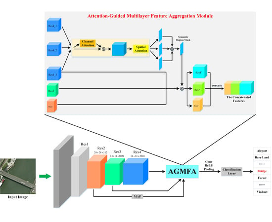
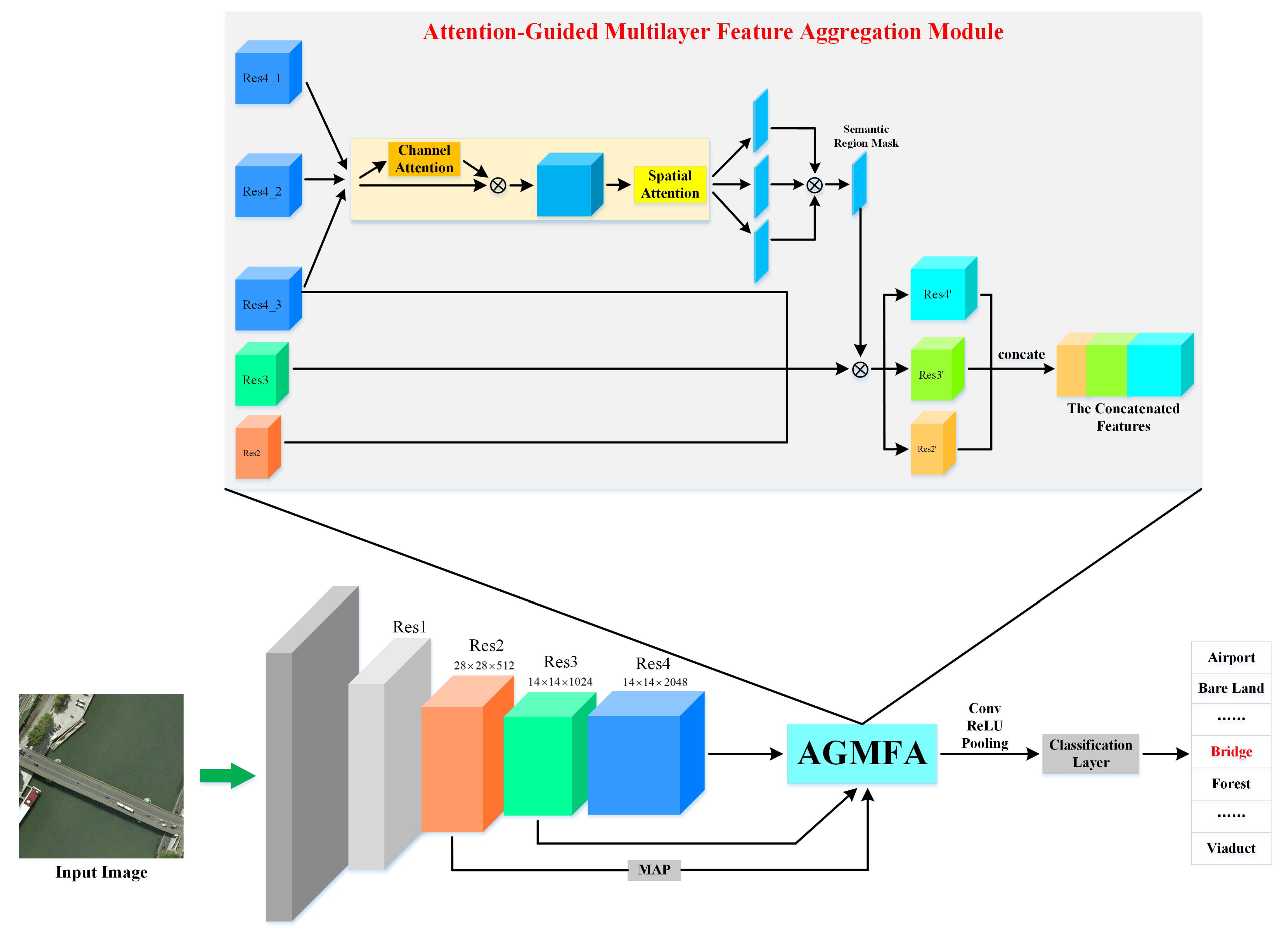
3.1. Overall Architecture

The goal of the proposed method is to learn discriminative feature representation for remote sensing image scene classification. Figure 2 illustrates the overall architecture of AGMFA-Net, which consists of three main components: feature extraction module, multilayer feature aggregation module, and classification module. Our network was built on ResNet-50 [15] as the backbone. Firstly, the input image is fed into the backbone to generate a series of convolutional feature maps that contain different levels of information about the given scene; we denote them as Res 2 , Res 3 , Res 4 _ 1 , Res 4 _ 2 , and Res 4 _ 3 . Then, the multilayer feature aggregation module is utilized to fuse these features to generate a new feature with more powerful scene representation ability. Concretely, in order to achieve semantic regions corresponding to the given scene as accurately as possible, the channel–spatial attention module was simultaneously employed on multiple high-level feature maps, i.e., Res 4 _ 1 , Res 4 _ 2 , and Res 4 _ 3 , and a new attention mask is generated. Then, we used this mask to guide the multilayer feature aggregation procedure. Through this process, discriminative information of different feature maps will be well fused to generate a more powerful scene representation, as well as suppress some interference or useless information caused by low-level feature maps. After that, a block operation (including convolution, ReLU, normalization) was employed to merge the information of the aggregated features among the channel. Finally, a fully connected layer and a softmax layer followed to predict the label of the input scene. In the following subsections, we introduce each component in detail.

3.2. Multilayer Feature Extraction

Limited by the scarcity of training samples in remote sensing images, many existing methods capture multilayer convolutional features using the pretrained CNN models. Currently, many famous CNN architectures have been developed, e.g., AlexNet, VGGNet, ResNet, etc. Considering the excellent classification performance of ResNet on ImageNet, in this paper, we used the modified ResNet-50 to extract multilayer convolutional feature maps from remote sensing scenes. For the ResNet-50 model, it starts with an initial convolutional layer with a kernel of size 7 × 7 and a stride of 2. Then, a max-pooling layer is added with a 3 × 3 window and a stride of 2. The later portion is composed of four residual blocks; we denote the outputs of each residual block as Res 1 , Res 2 , Res 3 , and Res 4 , respectively. Because we only extracted multilayer feature maps, we deleted all layers after Res4. In addition, to retain more spatial information, we changed the stride of Res 4 from 2 to 1. Assuming the size of the input image is 3 × 224 × 224, the sizes of Res 2 , Res 3 , and Res 4 are 512 × 28 × 28, 1024 × 14 × 14, and 2048 × 14 × 14, respectively. At the same time, the size of high-level convolutional feature maps (e.g., Res 4 _ 1 , Res 4 _ 2 , and Res 4 _ 3 ) was the same, i.e., 512 × 14 × 14. It is worth noting that Res 4 and Res 4 _ 3 denote the same feature map; they both represent the output of the last residual block of ResNet-50. To ensure that the size of each feature map is consistent, we downsampled Res 2 to change its size to 512 × 14 × 14 by using a max-pooling operation. The main motivation to extract multilayer convolutional features was that they can complement each other, which has been proven to be helpful for improving the remote sensing image scene classification accuracy.

3.3. Multilayer Feature Aggregation

In general, the features from deeper layers can describe the semantic information of the given scenes better, while the features from lower layers have rich appearance information; they are both important for classification. Thus, fusing features from different layers has become a commonly used strategy to obtain a more comprehensive scene representation. However, directly aggregating multilayer features without considering the discrepancies between them, e.g., feature redundancy, semantic ambiguity, and background interference, may result in reducing the discriminative ability. To aggregate multilayer convolutional features more effectively and obtain more valuable information of each feature map, an attention-guided multilayer feature aggregation module was designed, as shown in Figure 2. It mainly consists of two parts: semantic region extraction and multilayer feature aggregation.
To reduce the impacts of semantic interference, feature redundancy, etc., between different convolutional layers, we followed a rule that only aggregates multilayer features corresponding to the semantic regions of the given scene. Therefore, there are two key issues that need to be considered: (1) how to accurately obtain the semantic regions of the input scenes; (2) how to fuse different levels of feature maps based on the learned semantic regions?

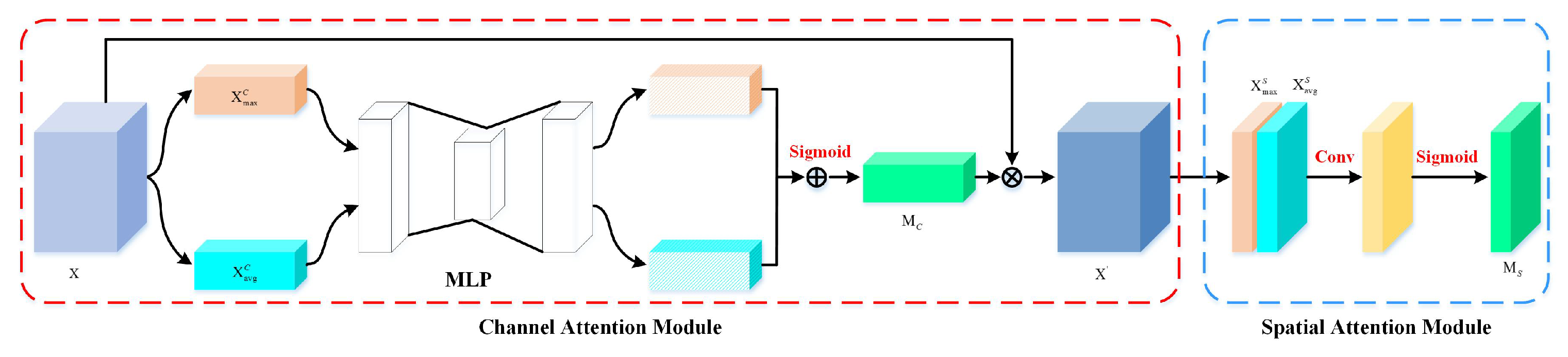
3.3.1. Semantic Region Extraction

For the first issue, a commonly used solution is to only use the last convolutional activation as the semantic regions. However, this solution is not effective because the semantic regions are incomplete and ignore other discriminative regions, which are also important for scene classification. To address this problem, we first analyzed the activation characteristics of different high-level convolutional feature maps in the last residual block of ResNet-50, and the visualization results are shown in Figure 3 by using the gradient-weighted class activation mapping (Grad-CAM) algorithm [64]. It can be observed that a single convolutional feature map usually only activates the most discriminative regions of the given scene, while ignoring the importance of other semantic areas. In addition, the activation regions of different convolutional feature maps are different, but also overlap. Furthermore, multiple convolutional feature maps can compensate each other to achieve more complete activation regions.
In order to capture more semantic regions of the given scene accurately, we proposed to simultaneously aggregate multiple high-level convolutional features based on the channel–spatial attention mechanism. Recently, benefiting from the human visual system, various attention mechanisms have been developed and have achieved great success in many fields, which aim to selectively concentrate on the prominent regions to extract the discriminative features from the given scene while discarding other interference information. Among them, the CBAM [55] algorithm is excellent and has been introduced in remote sensing scene classification. CBAM considers two different dimensions of the channel and spatial information simultaneously to capture important features and suppress useless features more effectively. Therefore, we employed CBAM in this paper to obtain important semantic regions from each high-level convolutional feature map.
Suppose Res 4 _ 1 R C × H × W , Res 4 _ 2 R C × H × W , and Res 4 _ 3 R C × H × W denote three high-level convolutional feature maps from the last residual block of ResNet-50, respectively. C, H, and W represent the channel number, height, and width of each feature map. As shown in Figure 2, each high-level convolutional feature map is first separately passed to the channel–spatial attention module to generate three different attention masks, and these masks are then multiplied to obtain the final semantic regions.
Figure 4 demonstrates the detailed workflow of the channel–spatial attention operation, which consists of two components: the channel stream and the spatial stream. Let the input feature map be X R C × H × W , where C, H, and W are the number of channels, height, and width, respectively. Firstly, two pooling operations, i.e., global max pooling and global average pooling, are employed to aggregate the spatial information of X and generate two C× 1 × 1 spatial contextual descriptors; we denote them as X max C R C × 1 × 1 and X avg C R C × 1 × 1 , respectively. Then, two descriptors are fed into a shared network with a hidden layer and multilayer perception. To reduce the computational overhead, the activation size of the hidden layer is R C / r × 1 × 1 , where r is the reduction ratio. After that, two output features of the shared network are added after a sigmoid activation function to obtain the channel attention map M C R C × 1 × 1 . Finally, the refined feature X is obtained by multiplying M C with the input feature map X. In summary, the entire process of channel attention can be expressed as follows:
X = M c ( X ) X
where ⊗ represents elementwise multiplication and M c X denotes the channel attention map, which can be described as:
M C ( X ) = σ ( MLP ( AvgPool ( X ) ) + MLP ( MaxPool ( X ) ) ) = σ ( W 1 ( W 0 ( X a v g C ) ) + W 1 ( W 0 ( X max C ) ) )
where σ denotes the sigmoid function, MLP represents the multi-layer perceptron, AvgPool and MaxPool denote the global average pooling and global max pooling, respectively, and W 0 R C / r × C and W 1 R C × C / r are the weights of the MLP.
Different from channel attention, spatial attention aims to utilize the interspatial relationships of features to generate a spatial attention map, which mainly focuses on the discriminative areas. To obtain the spatial attention map M S R H × W , the average pooling and max pooling operations are adopted along the channel dimension at first to generate two 1 × H × W channel descriptors, which are denoted as X a v g S R 1 × H × W and X max S R 1 × H × W . Then, these two channel descriptors are concatenated to generate a new descriptor. After that, a 7 × 7 convolution and sigmoid function are used to capture a spatial attention map M S , which can highlight the important regions of the given scenes while suppressing other interference regions. It should be noted that we only need to generate the spatial attention map, instead of reweighting the input feature map X to generate a refined feature map. Therefore, the spatial attention is computed as:
M S ( X ) = σ ( f 7 × 7 concat [ AvgPool ( X ) ; MaxPool ( X ) ] ) = σ ( f 7 × 7 concat [ X a v g S ; X m a x S ] )
where σ and concat denote the sigmoid function and concatenation operation, respectively, f 7 × 7 represents a convolution operation with a filter size of 7 × 7, and AvgPool and MaxPool represent the average pooling and max pooling along the channel dimension. By referring to [55], we connected channel attention and spatial attention in a sequential arrangement manner, which can more effectively focus on important semantic regions of the given scene.
For high-level convolutional feature maps, Res4_1, Res4_2, and Res4_3, we separately pass them into the channel–spatial attention module to capture different attention masks, denoted as M4_1, M4_2, and M4_3. It is worth noting that each mask mainly concentrates on discriminative regions, but they complement each other. To obtain a more accurate semantic region mask, we conducted the matrix multiplication operation on the above three masks, and the newly generated semantic region mask is denoted as M. Compared with the discriminative mask only using the last convolutional features of ResNet-50, our method makes full use of the information from multiple high-level convolutional feature maps to obtain a more efficient and complete semantic region mask, as shown in the last column in Figure 3. The expression of this procedure can be written as follows.
M = M 4 _ 1 M 4 _ 2 M 4 _ 3
where ⊗ denotes the elementwise multiplication operation.

3.3.2. Multilayer Feature Aggregation

It is acknowledged that convolutional features extracted from different layers can describe different levels of information of the given scene; some published research [6,33,38] has also proven that fusing multiple convolutional features can significantly promote the scene classification performance. However, integrating multilayer convolutional features indiscriminately may be easily affected by the differences, e.g., semantic ambiguity, feature redundancy, and background interference, resulting in the discrimination of the learned scene representation being insufficient. To solve this problem, we designed a novel multilayer feature fusion strategy. Specifically, we first obtained semantic regions in terms of the semantic region extraction operation, then used the learned semantic regions to guide the process of multilayer feature aggregation. Compared with other fusion strategies, e.g., fusion by addition, our method not only fuses valuable feature information of each convolutional layer effectively, but also avoids the interference of unfavorable factors.
As shown in Figure 2, Res 2 , Res 3 , and Res 4 are three different convolutional feature maps captured from the backbone network. M represents the semantic region mask. To aggregate multilayer convolutional features, we separately multiply Res 2 , Res 3 , and Res 4 by M to generate new features; we present them as Res 2 , Res 3 , and Res 4 . By this step, different convolutional layers’ important information, which is consistent with M, is selected for the subsequent fusion procedure. After that, these features are concatenated along the channel dimension. Specifically, in order to reduce the feature dimension and merge the information of the concatenated features among the channels, a 1 × 1 convolution operation and a ReLU operation are followed; we denote the output features as Y. Therefore, we can use the formula to express this as follows:
Re s 2 = Re s 2 M Re s 3 = Re s 3 M Re s 4 = Re s 4 M Y = δ ( f 1 × 1 concat [ Res 2 ; Re s 3 ; Re s 4 ] )
where ⊗ denotes the elementwise operation, δ represents the ReLU function, f 1 × 1 denotes a convolution operation with the filter size of 1 × 1, and concat represents the concatenation operation.
After obtaining Y, it is sent into the classifier for scene classification.

3.4. Loss Function

During training, the cross entropy loss function is used to minimize a weighted cumulation loss. Suppose that I = x 1 , y 1 , . . . , x N , y N is a training batch of N images, where y i , a one-hot vector, is the label of the i-th image x i . p i is a vector in which the j-th element is the probability that image x i is classified into the j-th class. Then, the cross entropy loss can be formulated as follows:
L = 1 N i = 1 N y i I log p i

4. Experiments

In this section, we conduct a series of experiments to verify the effectiveness of the proposed AGMFA-Net.

4.1. Datasets

To evaluate the performance of the proposed method, the following commonly used remote sensing scene classification datasets were employed: the UC Merced Land Use dataset [30], the more challenging large-scale Aerial Image Dataset (AID) [18], and the NWPU-RESISC45 dataset [17].
(1) UC Merced Land Use dataset (UCML): The UCML dataset is a classical benchmark for remote sensing scene classification. It consists of 21 different classes of land use images with a pixel resolution of 0.3 m. It contains a total of 2100 remote sensing images with 100 samples for each class. These samples are all annotated from a publicly available aerial image, and the size of each sample is 256 × 256 pixels. The example images of each class are shown in Figure 5.
(2) Aerial Image Dataset (AID): The AID dataset has 10,000 remote sensing scene images, which are divided into 30 different land cover categories. Each category’s number varies from 220 to 420. The size of each image is 600 × 600 pixels, and the spatial resolution ranges from about 8 m to 0.5 m. It is noted that the AID dataset is a relatively large-scale remote sensing scene dataset and is challenging for classifying. Some examples of each category are presented in Figure 6.
(3) NWPU-RESISC45 dataset: This dataset is more complex and challenging compared with the above three datasets. It contains a total of 31,500 images divided into 45 different scenes. Each scene has 700 images with an image size of 256 × 256 pixels. Because of the more diverse scenes, the spatial resolution of the images varies from 0.2 m to 30 m. Figure 7 shows some examples of this dataset.
To ensure a fair comparison, we employed the commonly used training ratios to divide each dataset. For the UCML dataset, we set the training ratio to 80% and the rest of the samples (20%) for testing. For the AID dataset, we set two training–testing ratios, i.e., 20–80% and 50–50%, respectively. Similarly, two training ratios, i.e., 10–90% and 20–80%, were used for the NWPU-RESISC45 dataset.

4.2. Implementation Details

All experiments were completed using the PyTorch [65] deep learning library. We employed ResNet-50 as the backbone network. To verify the scalability of the proposed method, we also conducted experiments with the VGGNet-16 network. All networks were trained using one NVIDIA GeForce RTX 2070 Super GPU. To make the network converge quickly, all the experimental networks were first pretrained on the ImageNet and then fine-tuned with the above three benchmark datasets. Our proposed network was optimized by the stochastic gradient descent (SGD) algorithm with the momentum as 0.9, the initial learning as 0.001, and the weight decay penalty as 1 × 10⁻⁵. After every 30 epochs, the learning rate decayed by 10 times. The batch size and maximum training iterations were set to 32 and 150, respectively. In the training stage, data augmentation was adopted to improve the generalization performance. Concretely, the input images were first resized to 256 × 256 pixels, then randomly cropped to 224 × 224 pixels as the network input after random horizontal flipping.

4.3. Evaluation Metrics

To comprehensively evaluate the classification of the proposed method, three evaluation metrics were used in this paper. They include the overall accuracy and the confusion matrix. Each evaluation metric is explained as follows:
(1) Overall accuracy (OA): The OA is defined as the ratio between the number of correctly classified images and the total number of testing images;
(2) Confusion matrix (CM): The CM is a special matrix used to visually evaluate the performance of the algorithm. In this matrix, the column represents the ground truth and the row denotes the prediction. From it, we can observe the classification accuracy of each scene, as well as the categories that are easily confused with each other.

4.4. Ablation Study

In our proposed method, we mainly improved the discriminative capability of the multilayer feature aggregation from two aspects. To separately demonstrate the effectiveness of each component, we conducted ablation experiments on the AID and NWPU-RESISC45 datasets using ResNet-50 as the backbone network.

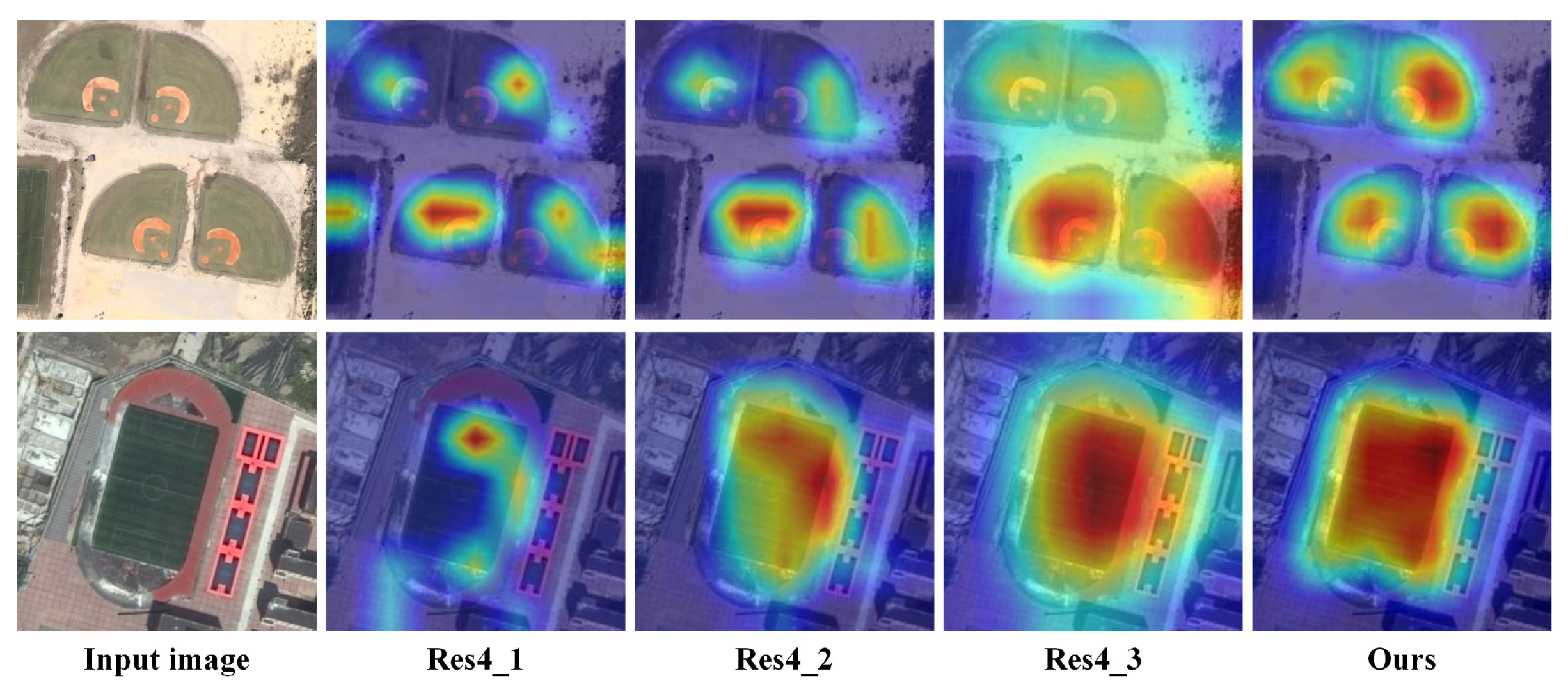
4.4.1. The Effectiveness of Semantic Region Extraction

We conducted experiments to qualitatively analyze the effectiveness of semantic region extraction. In the following, we compare the following network architectures, i.e., ResNet-50, ResNet-50+DA (direct aggregation), ResNet-50+WA (without attention), ResNet-50+SA (spatial attention), Ours (low-level features), Ours (multiple high-level features). Specifically, ResNet-50 was the baseline network. ResNet-50+DA represents directly aggregating multiple high-level convolutional feature maps indiscriminately. ResNet-50+WA denotes aggregating multiple high-level convolutional feature maps without using attention. Instead, we employed the method in [66], which captures semantic regions by utilizing multiple high-level convolutional feature maps in an unsupervised way. ResNet-50+SA represents using the spatial attention following each high-level convolutional feature map, then aggregating them to generate new semantic regions. Ours (low-level features) and Ours (high-level features) are two methods that adopt channel attention and spatial attention separately on low-level and high-level features to capture semantic regions. More intuitively, we illustrate the activation maps of the aggregated features between different compared methods using the Grad-CAM algorithm in Figure 8. It can be observed that the above six methods can activate the discriminative regions, which are consistent with the semantic label of the scenes; however, the activation regions of our proposed method are more complete and can accurately cover the overall discriminative regions.

4.4.2. The Effectiveness of Multilayer Feature Aggregation

We also conducted experiments on the AID and NWPU-RESISC45 datasets to quantitatively evaluate the performance of the proposed multilayer feature aggregation strategy, and the results are shown in Table 1. From Table 1, we can make the following conclusions: (1) For the AID and NWPU-RESISC45 datasets, the multilayer feature aggregation methods can further promote the classification accuracy when compared with the baseline. This observation verified that fusing features from different layers can indeed achieve better results. (2) The classification accuracy of ResNet-50+DA and ResNet-50+WA was similar. We considered the reason is partly that ResNet-50+WA employs an unsupervised method to obtain semantic regions, which cannot suppress the impacts of complex backgrounds, resulting in worse accuracy. (3) The methods based on attention were better than ResNet-50+DA and ResNet-50+WA, except the training ratio of the NWPU-RESISC45 dataset was 10%. We also respectively compared the classification performance when obtaining semantic regions based on low-level and high-level features in our method. (4) We found that when using low-level features, its classification performance on the AID and NWPU-RESISC45 datasets was better than the baseline, but lower than other methods. We considered the reason to be that the use of low-level revolutionary features cannot effectively reduce the interference of background noise and semantic ambiguity, resulting in the captured semantic regions being inaccurate, which further reduces the performance of multilayer feature fusion. (5) When using multiple high-level convolutional features to capture semantic regions, our method can achieve optimal classification accuracy because we used channel and spatial attention together to obtain more accurate semantic regions. Therefore, the final aggregated features have better discrimination.

4.5. State-of-the-Art Comparison and Analysis

4.5.1. Results on the UCML Dataset

UCML is a classical dataset for evaluating the performance of remote sensing image scene classification. To illustrate the superiority of our proposed method, we compared it with some state-of-the-art scene classification methods that are reviewed in Section 2, and the comparison results are shown in Table 2. As can be seen from Table 2, our method, which employed ResNet-50 as the backbone, achieved the optimal overall classification accuracy. In addition, when using VGGNet-16, our method also surpassed most of the methods and obtained a competitive classification performance. It is worth noting that the overall accuracy of most of the compared methods reached above 98%, but our method still showed good superiority and demonstrated its effectiveness.
Figure 9 shows the confusion matrix of our proposed method when the training ratio was 80%. It can be seen that almost all scenes can be accurately classified except for some easily confused categories, such as freeway and overpass, medium residential and dense residential, and forest and sparse residential. This is because some scenes are composed of multiple different land use units (e.g., sparse residential contains forest and building together) or show different spatial layout characteristics (e.g., freeway and overpass both contain road, but they have different spatial layouts). These issues make them difficult to classify.

4.5.2. Results on the AID Dataset

AID is a larger and more challenging dataset than the UCML dataset. We compared our method with other scene classification methods with two training ratios, 20% and 50%. For both training ratios, our method performed better than other competitors, as shown in Table 3. For a training ratio of 50%, our method with VGGNet-16 as the backbone surpassed almost all the compared methods that use the same backbone, such as Fusion by Addition [25], VGG-16+MSCP [35], ARCNet-VGG16 [45], MF 2 Net [6], VGG-16-CapsNet [48], etc. Similarly, when using ResNet-50 as the backbone, our method achieved the highest classification accuracy, which exceeded other methods that use ResNet or more advanced network as the backbone. For example, our method increased by 0.06% over ResNet-50+EAM [47], 0.11 over IB-CNN (M) [51], and 0.12 over EfficientNet-B3-aux [50]. For a training ratio of 20%, our method that used VGGNet-16 showed mediocre performance; however, when using ResNet-50 as the backbone, our method performed better than all the other methods. Specifically, our method was slightly higher than EfficientNet-B3-aux and IB-CNN(M) by 0.16% and 0.02% and exceeded ResNet-50+EAM by 0.16%.
The CMs of different training ratios are illustrated in Figure 10 and Figure 11, respectively. For a training ratio of 50% in Figure 10, most of the categories achieved a classification accuracy higher than 95%, except the scenes of resort (92%) and school (93%). Specifically, the most difficult scenes to classify were resort and park, because they are composed of some similar land use units and also have the same spatial structures. In addition, school is easily confused with square and industrial. For a training ratio of 20% in Figure 11, our method can also obtain excellent classification accuracy, except for the following four scenes: center (87%), resort (79%), school (84%), and square (86%).

4.5.3. Results on the NWPU-RESISC45 Dataset

For the larger NWPU-RESISC45 dataset, the comparison results are shown in Table 4. For two training ratios, our methods obtained remarkable performance. When the training ratio was 20%, our method that used ResNet-50 as the backbone exceeded all the competitors. Specifically, in comparison to the baselines, our method separately improved by 1.79% (ResNet-50) and 2.86% (VGGNet-16) when using different networks. When using VGGNet-16 as the backbone, we surpassed other methods that use the same backbone, e.g., Two-Stream [39], VGGNet16+MSCP, MF 2 Net , and VGG-16-CapsNet. In addition, our method achieved the highest classification accuracy when using ResNet-50, higher than ResNet-50+EAM by 0.19% and higher than IB-CNN (M) by 0.37%. For the training ratio of 10%, our methods can also obtain excellent classification performance.
Figure 12 and Figure 13 are the confusion matrix results for the training ratios of 20% and 10%, respectively. It can be observed that when setting the training ratio to 20%, almost all the scenes can achieve above 90% classification accuracy, except two scenes, i.e., church (83%) and palace (83%), which are very easily confused with each other. In addition, for the training ratio of 10%, most of the scenes can be classified well; the scenes with the lowest classification accuracy still remain church (77%) and palace (75%).

5. Conclusions

One of the crucial challenges of remote sensing image scene classification is how to learn a powerful scene representation. To address this problem, we presented a novel attention-guided multilayer feature aggregation network in this paper, which consisted of three parts: the multilayer feature extraction module, the multilayer feature aggregation module, and the classification module. Concretely, we first used the backbone network to extract multiple convolutional feature maps with different spatial resolutions. Then, a semantically guided multilayer feature aggregation module was used to integrate features from different convolutional layers to reduce the interferences of useless information and at the same time improve the scene representation capacity. Specifically, to capture semantic regions that were consistent with the given scene accurately, we employed channel–spatial attention to make full use of the feature information of multiple high-level convolutional feature layers. Compared with the semantic regions captured from a single convolutional layer, our method showed better results. Finally, the aggregated features were fed into the classifier for scene classification. Experiments on three benchmark datasets were conducted, and the results demonstrated that our proposed method can achieve promising classification performance and outperform other remote sensing image scene classification methods.

Author Contributions

Conceptualization, M.L.; data curation, M.L. and L.L.; formal analysis, M.L.; methodology, M.L. and Y.S.; software, M.L.; validation, M.L. and Y.S.; writing—original draft, M.L.; writing—review and editing, L.L., Y.T. and G.K. All authors read and agreed to the published version of the manuscript.

Funding

This research received no external funding.

Institutional Review Board Statement

Not applicable.

Informed Consent Statement

Not applicable.

Data Availability Statement

The UC Merced Land Use, AID and NWPU-RESISC45 datasets used in this study are openly and freely available at http://weegee.vision.ucmerced.edu/datasets/landuse.html, https://captain-whu.github.io/AID/, and https://gcheng-nwpu.github.io/datasets#RESISC45, respectively.

Acknowledgments

We would like to thank the handling Editor and the anonymous reviewers for their careful reading and helpful suggestions.

Conflicts of Interest

The authors declare no conflict of interest.

References

  1. Mou, L.; Ghamisi, P.; Zhu, X.X. Deep recurrent neural networks for hyperspectral image classification. IEEE Trans. Geosci. Remote Sens. 2017, 55, 3639–3655. [Google Scholar] [CrossRef] [Green Version]
  2. Li, X.; Lei, L.; Sun, Y.; Li, M.; Kuang, G. Multimodal bilinear fusion network with second-order attention-based channel selection for land cover classification. IEEE J. Sel. Top. Appl. Earth Obs. Remote Sens. 2020, 13, 1011–1026. [Google Scholar] [CrossRef]
  3. Wu, C.; Zhang, L.; Zhang, L. A scene change detection framework for multi-temporal very high resolution remote sensing images. Signal Process 2015, 124, 84–197. [Google Scholar] [CrossRef]
  4. Hu, Q.; Wu, W.; Xia, T.; Yu, Q.; Yang, P.; Li, Z.; Song, Q. Exploring the use of Google Earth imagery and object-based methods in land use/cover mapping. Remote Sens. 2013, 105, 6026–6042. [Google Scholar] [CrossRef] [Green Version]
  5. Wang, C.; Shi, J.; Yang, X.; Zhou, Y.; Wei, S.; Li, L.; Zhang, X. Geospatial object detection via deconvolutional region proposal network. IEEE J. Sel. Topics Appl. Earth Observ. Remote Sens. 2019, 12, 3014–3027. [Google Scholar] [CrossRef]
  6. Xu, K.; Huang, H.; Li, Y.; Shi, G. Multilayer feature fusion network for scene classification in remote sensing. IEEE Geosci. Remote Sens. Lett. 2020, 17, 1894–1898. [Google Scholar] [CrossRef]
  7. Swain, M.J.; Ballard, D.H. Color indexing. Int. J. Comput. Vis. 1991, 7, 11–32. [Google Scholar] [CrossRef]
  8. Haralick, R.M.; Shanmugam, K.; Dinstein, I.H. Textural features for image classification. IEEE Trans. Syst. Man Cybern. 1973, SMC-3, 610–621. [Google Scholar] [CrossRef] [Green Version]
  9. Lowe, D.G. Distinctive image features from scale-invariant key-points. Int. J. Comput. Vis. 2004, 60, 91–110. [Google Scholar] [CrossRef]
  10. Dalal, N.; Triggs, B. Histograms of oriented gradients for human detection. In Proceedings of the 2005 IEEE Computer Society Conference on Computer Vision and Pattern Recognition (CVPR’05), San Diego, CA, USA, 20–25 June 2005; Volume 1, pp. 886–893. [Google Scholar]
  11. Krizhevsky, A.; Sutskever, I.; Hinton, G. Imagenet classification with deep convolutional neural networks. Adv. Neural Inf. Process. Syst. 2012, 25, 1097–1105. [Google Scholar] [CrossRef]
  12. Simonyan, K.; Zisserman, A. Very deep convolutional networks for large-scale image recognition. arXiv 2014, arXiv:1409.1556. [Google Scholar]
  13. Ren, S.; He, K.; Girshick, R.; Sun, J. Faster R-CNN: Towards real-time object detection with region proposal networks. IEEE Trans. Pattern Anal. Mach. Intell 2017, 39, 1137–1149. [Google Scholar] [CrossRef] [PubMed] [Green Version]
  14. Chen, L.; Papandreou, G.; Kokkinos, I.; Murphy, K.; Yuille, A.L. DeepLab: Semantic image segmentation with deep convolutional nets, atrous convolution, and fully connected CRFs. IEEE Trans. Pattern Anal. Mach. Intell. 2018, 40, 834–848. [Google Scholar] [CrossRef] [PubMed]
  15. He, K.; Zhang, X.; Ren, S.; Sun, J. Deep residual learning for image recognition. In Proceedings of the 2016 IEEE Conference on Computer Vision and Pattern Recognition (CVPR), Las Vegas, NV, USA, 27–30 June 2016; pp. 770–778. [Google Scholar]
  16. Huang, G.; Liu, Z.; Van Der Maaten, L.; Weinberger, K.Q. Densely connected convolutional networks. In Proceedings of the IEEE Conference on Computer Vision and Pattern Recognition, Honolulu, HI, USA, 21–26 July 2017; pp. 2261–2269. [Google Scholar]
  17. Cheng, G.; Han, J.; Lu, X. Remote sensing image scene classification: Benchmark and state of the art. Proc. IEEE 2017, 105, 1865–1883. [Google Scholar] [CrossRef] [Green Version]
  18. Xia, G.-S.; Hu, J.; Hu, F.; Shi, B.; Bai, X.; Zhong, Y.; Zhang, L.; Lu, X. AID: A benchmark data set for performance evaluation of aerial scene classification. IEEE Trans. Geosci. Remote Sens. 2017, 55, 3965–3981. [Google Scholar] [CrossRef] [Green Version]
  19. Cheng, G.; Xie, X.; Han, J.; Guo, L.; Xia, G.S. Remote sensing image scene classification meets deep learning: Challenges, methods, benchmarks, and opportunities. IEEE J. Sel. Topics. Appl. Earth Observ. Remote Sens. 2020, 13, 3735–3756. [Google Scholar] [CrossRef]
  20. Nogueira, K.; Penatti, O.A.; Santos, J.A.D. Towards better exploiting convolutional neural networks for remote sensing scene classification. Pattern Recognit 2017, 61, 539–556. [Google Scholar] [CrossRef] [Green Version]
  21. Cheng, G.; Li, Z.; Yao, X.; Guo, L.; Wei, Z. Remote sensing image scene classification using bag of convolutional features. IEEE Geosci. Remote Sens. Lett. 2017, 14, 1735–1739. [Google Scholar] [CrossRef]
  22. Wang, S.; Guan, Y.; Shao, L. Multi-granularity canonical appearance pooling for remote sensing scene classification. IEEE Trans. Image Process 2020, 29, 5396–5407. [Google Scholar] [CrossRef] [Green Version]
  23. Li, E.; Xia, J.; Du, P.; Lin, C.; Samat, A. Integrating multilayer features of convolutional neural networks for remote sensing scene classification. IEEE Trans. Geosci. Remote Sens. 2017, 55, 5653–5665. [Google Scholar] [CrossRef]
  24. Lu, X.; Sun, H.; Zheng, X. A feature aggregation convolutional neural network for remote sensing scene classification. IEEE Trans. Geosci. Remote Sens. 2019, 57, 7894–7906. [Google Scholar] [CrossRef]
  25. Chaib, S.; Liu, H.; Gu, Y.; Yao, H. Deep feature fusion for VHR remote sensing scene classification. IEEE Trans. Geosci. Remote Sens. 2017, 55, 4775–4784. [Google Scholar] [CrossRef]
  26. Deng, J.; Dong, W.; Socher, R.; Li, L.-J.; Li, K.; Fei-Fei, L. ImageNet: A large-scale hierarchical image database. In Proceedings of the 2009 IEEE Conference on Computer Vision and Pattern Recognition, Miami, FL, USA, 20–25 June 2009; pp. 248–255. [Google Scholar]
  27. Liang, Y.; Monteiro, S.T.; Saber, E.S. Transfer learning for high resolution aerial image classification. In Proceedings of the 2016 IEEE Applied Imagery Pattern Recognition Workshop (AIPR), Washington, DC, USA, 18–20 October 2016; pp. 1–8. [Google Scholar]
  28. Szegedy, C.; Liu, W.; Jia, Y.; Sermanet, P.; Reed, S.; Anguelov, D.; Erhan, D.; Vanhoucke, V.; Rabinovich, A. Going deeper with convolutions. In Proceedings of the 2015 IEEE Conference on Computer Vision and Pattern Recognition (CVPR), Boston, MA, USA, 7–12 June 2015; pp. 1–9.
  29. Zhao, W.; Du, S. Scene classification using multi-scale deeply described visual words. Int. J. Remote Sens. 2016, 37, 4119–4131. [Google Scholar] [CrossRef]
  30. Yang, Y.; Newsam, S. Bag-of-visual-words and spatial extensions for land use classification. In Proceedings of the GIS ’10: 18th Sigspatial International Conference on Advances in Geographic Information Systems, San Jose, CA, USA, 2–5 November 2010; ACM: New York, NY, USA, 2010; pp. 270–279. [Google Scholar]
  31. Zheng, X.; Yuan, Y.; Lu, X. A deep scene representation for aerial scene classification. IEEE Trans. Geosci. Remote Sens. 2019, 57, 4799–4809. [Google Scholar] [CrossRef]
  32. Sanchez, J.; Perronnin, F.; Mensink, T.; Verbeek, J. Image classification with the fisher vector: Theory and practice. Int. J. Comput. Vis. 2013, 105, 222–245. [Google Scholar] [CrossRef]
  33. Wang, G.; Fan, B.; Xiang, S.; Pan, C. Aggregating rich hierarchical features for scene classification in remote sensing imagery. IEEE J. Sel. Topics. Appl. Earth Observ. Remote Sens. 2017, 10, 4104–4115. [Google Scholar] [CrossRef]
  34. Negrel, R.; Picard, D.; Gosselin, P.-H. Evaluation of second-order visual features for land use classification. In Proceedings of the 2014 12th International Workshop on Content-Based Multimedia Indexing (CBMI), Klagenfurt, Austria, 18–20 June 2014; pp. 1–5. [Google Scholar]
  35. He, N.; Fang, L.; Li, S.; Plaza, A.; Plaza, J. Remote sensing scene classification using multilayer stacked covariance pooling. IEEE Trans. Geosci. Remote Sens. 2018, 56, 6899–6910. [Google Scholar] [CrossRef]
  36. Lu, X.; Ji, W.; Li, X.; Zheng, X. Bidirectional adaptive feature fusion for remote sensing scene classification. Neurocomputing 2019, 328, 135–146. [Google Scholar] [CrossRef]
  37. Yu, Y.; Liu, F. Dense connectivity based two-stream deep feature fusion framework for aerial scene classification. Remote Sens. 2018, 10, 1158. [Google Scholar] [CrossRef] [Green Version]
  38. Sun, H.; Li, S.; Zheng, X.; Lu, X. Remote sensing scene classification by gated bidirectional network. IEEE Trans. Geosci. Remote Sens. 2020, 58, 82–96. [Google Scholar] [CrossRef]
  39. Yu, Y.; Liu, F. A two-stream deep fusion framework for high-resolution aerial scene classification. Comput. Intell. Neurosci. 2018, 2018, 8639367. [Google Scholar] [CrossRef] [PubMed] [Green Version]
  40. Yu, Y.; Liu, F. Aerial scene classification via multilevel fusion based on deep convolutional neural networks. IEEE Geosci. Remote Sens. Lett. 2018, 15, 287–291. [Google Scholar] [CrossRef]
  41. Du, P.; Li, E.; Xia, J.; Samat, A.; Bai, X. Feature and model level fusion of pretrained CNN for remote sensing scene classification. IEEE J. Sel. Topics Appl. Earth Observ. Remote Sens. 2019, 12, 2600–2611. [Google Scholar] [CrossRef]
  42. Zeng, D.; Chen, S.; Chen, B.; Li, S. Improving remote sensing scene classification by integrating global-context and local-object features. Remote Sens. 2018, 10, 734. [Google Scholar] [CrossRef] [Green Version]
  43. Liu, Y.; Zhong, Y.; Qin, Q. Scene classification based on multiscale convolutional neural network. IEEE Trans. Geosci. Remote Sens. 2018, 56, 7109–7121. [Google Scholar] [CrossRef] [Green Version]
  44. Ji, J.; Zhang, T.; Jiang, L.; Zhong, W.; Xiong, H. Combining multilevel features for remote sensing image scene classification with attention model. IEEE Geosci. Remote Sens. Lett. 2020, 17, 1647–1651. [Google Scholar] [CrossRef]
  45. Wang, Q.; Liu, S.; Chanussot, J.; Li, X. Scene classification with recurrent attention of VHR remote sensing images. IEEE Trans. Geosci. Remote Sens. 2019, 57, 1155–1167. [Google Scholar] [CrossRef]
  46. Cao, R.; Fang, L.; Lu, T.; He, N. Self-attention-based deep feature fusion for remote sensing scene classification. IEEE Geosci. Remote Sens. Lett. 2021, 18, 43–47. [Google Scholar] [CrossRef]
  47. Zhao, Z.; Li, J.; Luo, Z.; Li, J.; Chen, C. Remote sensing image scene classification based on an enhanced attention module. IEEE Geosci. Remote Sens. Lett. 2020. [Google Scholar] [CrossRef]
  48. Zhang, W.; Tang, P.; Zhao, L. Remote sensing image scene classification using CNN-CapsNet. Remote Sens. 2019, 11, 494. [Google Scholar] [CrossRef] [Green Version]
  49. Yu, Y.; Li, X.; Liu, F. Attention GANs: Unsupervised deep feature learning for aerial scene classification. IEEE Trans. Geosci. Remote Sens. 2020, 58, 519–531. [Google Scholar] [CrossRef]
  50. Bazi, Y.; Rahhal, A.; Alhichri, M.M.H.; Alajlan, N. Simple yet effective fine-tuning of deep CNNs using an auxiliary classification loss for remote sensing scene classification. Remote Sens. 2019, 11, 2908. [Google Scholar] [CrossRef] [Green Version]
  51. Li, E.; Samat, A.; Du, P.; Liu, W.; Hu, J. Improved Bilinear CNN Model for Remote Sensing Scene Classification. IEEE Geosci. Remote Sens. Lett. 2020. [Google Scholar] [CrossRef]
  52. Peng, C.; Li, Y.; Jiao, L.; Shang, R. Efficient Convolutional Neural Architecture Search for Remote Sensing Image Scene Classification. IEEE Trans. Geosci. Remote Sens. 2021, 59, 6092–6105. [Google Scholar] [CrossRef]
  53. Zhang, P.; Bai, Y.; Wang, D.; Bai, B.; Li, Y. Few-shot classification of aerial scene images via meta-learning. Remote Sens. 2021, 13, 108. [Google Scholar] [CrossRef]
  54. Hu, J.; Shen, L.; Sun, G. Squeeze-and-excitation networks. In Proceedings of the 2018 IEEE/CVF Conference on Computer Vision and Pattern Recognition, Salt Lake City, UT, USA, 18–23 June 2018; pp. 7132–7141. [Google Scholar]
  55. Woo, S.; Park, J.; Lee, J.Y. Cbam: Convolutional block attention module. In Proceedings of the European Conference on Computer Vision, Munich, Germany, 8–14 September 2018; pp. 3–19. [Google Scholar]
  56. Wang, X.; Girshick, R.; Gupta, A.; He, K. Non-local neural networks. In Proceedings of the 2018 IEEE/CVF Conference on Computer Vision and Pattern Recognition Workshops (CVPRW), Salt Lake City, UT, USA, 18–22 June 2018; pp. 7794–7803. [Google Scholar]
  57. Vaswani, A.; Shazeer, N.; Parmar, N.; Uszkoreit, J.; Jones, L.; Gomez, A.N.; Kaiser, L.; Polosukhin, I. Attention is all you need. In Proceedings of the Advances in Neural Information Processing Systems, Long Beach, CA, USA, 4–9 December 2017; pp. 5998–6008.
  58. Gu, Y.; Wang, L.; Wang, Z.; Liu, Y.; Cheng, M.-M.; Lu, S.-P. Pyramid Constrained Selfw-Attention Network for Fast Video Salient Object Detection. Proc. AAAI Conf. Artif. Intell 2020, 34, 10869–10876. [Google Scholar]
  59. Zhu, F.; Fang, C.; Ma, K.-K. PNEN: Pyramid Non-Local Enhanced Networks. IEEE Trans. Image Process. 2020, 29, 8831–8841. [Google Scholar] [CrossRef]
  60. Cao, Y.; Xu, J.; Lin, S.; Wei, F.; Hu, H. GCNet: Non-local networks meet squeeze-excitation networks and beyond. In Proceedings of the 2019 IEEE/CVF International Conference on Computer Vision Workshops, ICCV Workshops 2019, Seoul, Korea, 27–28 October 2019; pp. 1971–1980. [Google Scholar]
  61. Huang, Z.; Wang, X.; Huang, L.; Huang, C.; Wei, Y.; Liu, W. CCNet: Criss-cross attention for semantic segmentation. In Proceedings of the 2018 IEEE/CVF Conference on Computer Vision and Pattern Recognition (CVPR 2018), Salt Lake City, UT, USA, 18–22 June 2018; pp. 603–612. [Google Scholar]
  62. Zhang, D.; Li, N.; Ye, Q. Positional context aggregation network for remote sensing scene classification. IEEE Geosci. Remote Sens. Lett. 2020, 17, 943–947. [Google Scholar] [CrossRef]
  63. Fu, L.; Zhang, D.; Ye, Q. Recurrent Thrifty Attention Network for Remote Sensing Scene Recognition. IEEE Trans. Geosci. Remote Sens. 2020. [Google Scholar] [CrossRef]
  64. Selvaraju, R.R.; Cogswell, M.; Das, A.; Vedantam, R.; Parikh, D.; Batra, D. Grad-CAM: Visual explanations from deep networks via gradient-based localization. In Proceedings of the 2017 IEEE International Conference on Computer Vision (ICCV), Venice, Italy, 22–29 October 2017; pp. 618–626. [Google Scholar]
  65. Paszke, A.; Gross, S.; Massa, F.; Lerer, A.; Bradbury, J.; Chanan, G.; Killeen, T.; Lin, Z.; Gimelshein, N.; Antiga, L.; et al. PyTorch: An imperative style, high-performance deep learning library. In Proceedings of the Advances in Neural Information Processing Systems, Vancouver, BC, Canada, 8–14 December 2019; pp. 8024–8035. [Google Scholar]
  66. Wei, X.; Luo, J.; Wu, J.; Zhou, Z. Selective convolution descriptor aggregation for fine-grained image retrieval. IEEE Trans. Image Process 2017, 26, 2868–2881. [Google Scholar] [CrossRef] [Green Version]
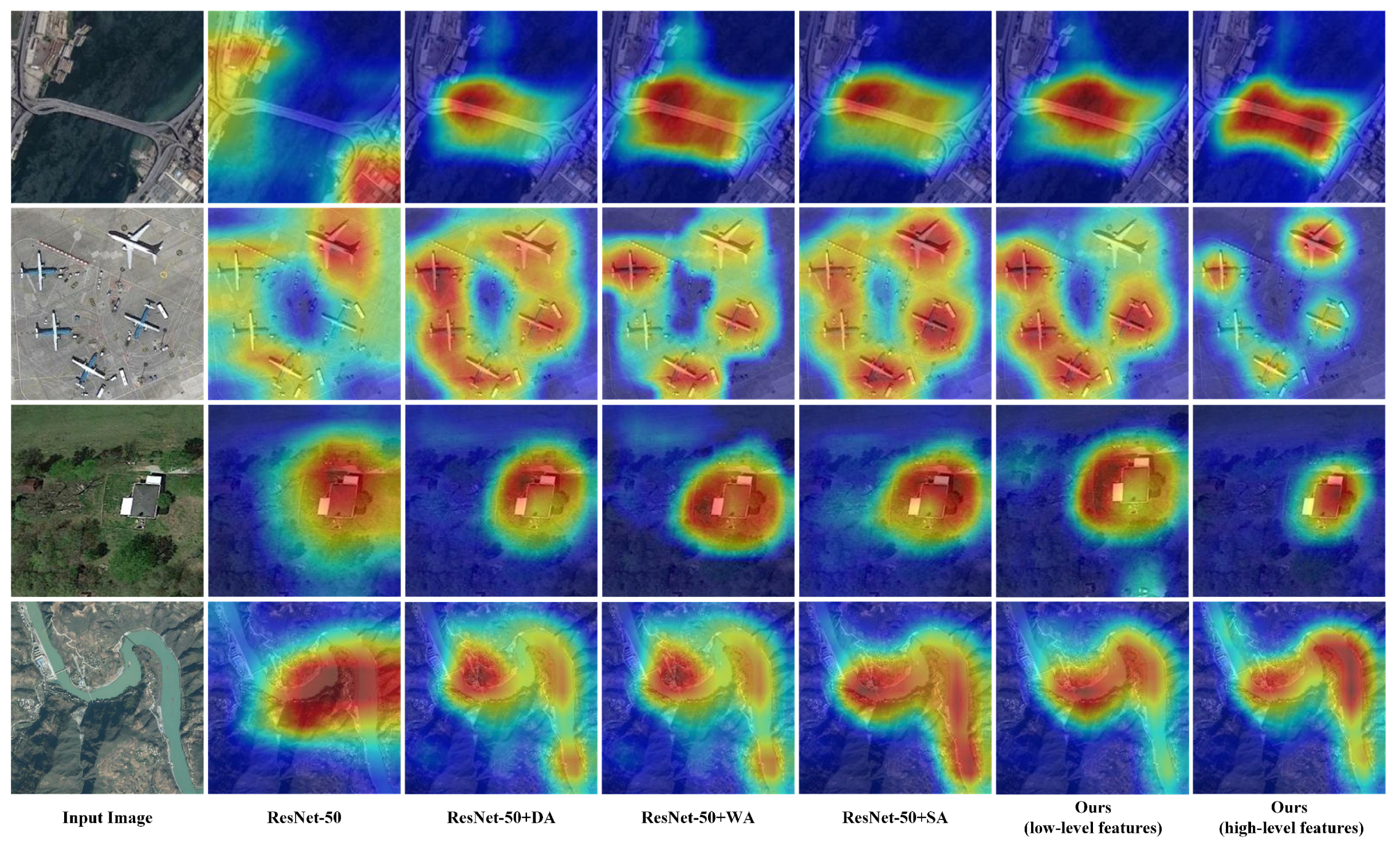
Figure 1. The characteristics of a remote sensing scene image. A remote sensing scene consists of many types of land cover units. However, to classify this scene, we only need to pay more attention to the key regions, i.e., bridge, while other regions can be regarded as interference.
Remotesensing 13 03113 g001
Figure 2. The overall architecture of our proposed AGMFA-Net.
Remotesensing 13 03113 g002
Figure 3. Grad-CAM visualization results. We compare the visualization results of our proposed channel–spatial attention with three other high-level convolutional feature maps of the last residual block of ResNet-50.
Remotesensing 13 03113 g003
Figure 4. Diagram of the channel–spatial attention module.
Remotesensing 13 03113 g004
Figure 5. Examples of the UCML dataset.
Remotesensing 13 03113 g005
Figure 6. Examples of the AID dataset.
Remotesensing 13 03113 g006
Figure 7. Examples of the NWPU-RESISC45 dataset.
Remotesensing 13 03113 g007
Figure 8. Grad-CAM visualization results. We compare the visualization results of the proposed AGMFA-Net (ResNet-50) with the baseline (ResNet-50) and three other multilayer feature aggregation methods. The Grad-CAM visualization is computed for the last convolutional outputs.
Remotesensing 13 03113 g008
Figure 9. Confusion matrix of the proposed method on the UCML dataset with a training ratio of 80%.
Remotesensing 13 03113 g009
Figure 10. Confusion matrix of the proposed method on the AID dataset with a training ratio of 50%.
Remotesensing 13 03113 g010
Figure 11. Confusion matrix of the proposed method on the AID dataset with a training ratio of 20%.
Remotesensing 13 03113 g011
Figure 12. Confusion matrix of the proposed method on the NWPU-RESISC45 dataset with a training ratio of 20%.
Remotesensing 13 03113 g012
Figure 13. Confusion matrix of the proposed method on the NWPU-RESISC45 dataset with a training ratio of 10%.
Remotesensing 13 03113 g013
Table 1. Ablation experimental results on two datasets with different training ratios.
MethodAIDNWPU-RESISC45
20%50%10%20%
ResNet-50 (Baseline)92.93 ± 0.2595.40 ± 0.1889.06 ± 0.3491.91 ± 0.09
ResNet-50+DA93.54 ± 0.3096.08 ± 0.3490.26 ± 0.0493.21 ± 0.16
ResNet-50+WA93.66 ± 0.2896.15 ± 0.2890.24 ± 0.0793.08 ± 0.04
ResNet-50+SA93.77 ± 0.3196.32 ± 0.1890.13 ± 0.5993.22 ± 0.10
Ours (low-level features)93.51 ± 0.5195.98 ± 0.2089.16 ± 0.3692.76 ± 0.11
Ours (high-level features)94.25 ± 0.1396.68 ± 0.2191.01 ± 0.1893.70 ± 0.08
Table 2. The OA (%) and STD (%) of different methods on the UCML dataset.
MethodsAccuracy
VGGNet-16 [12]96.10 ± 0.46
ResNet-50 [15]98.76 ± 0.20
MCNN [43]96.66 ± 0.90
Multi-CNN [41]99.05 ± 0.48
Fusion by Addition [25]97.42 ± 1.79
Two-Stream Fusion [39]98.02 ± 1.03
VGG-VD16+MSCP [35]98.40 ± 0.34
VGG-VD16+MSCP+MRA [35]98.40 ± 0.34
ARCNet-VGG16 [45]99.12 ± 0.40
VGG-16-CapsNet [48]98.81 ± 0.22
MG-CAP (Bilinear) [22]98.60 ± 0.26
MG-CAP (Sqrt-E) [22]99.00 ± 0.10
GBNet+global feature [38]98.57 ± 0.48
EfficientNet-B0-aux [50]99.04 ± 0.33
EfficientNet-B3-aux [50]99.09 ± 0.17
IB-CNN(M) [51]98.90 ± 0.21
TEX-TS-Net [37]98.40 ± 0.76
SAL-TS-Net [37]98.90 ± 0.95
ResNet-50+EAM [47]98.98 ± 0.37
Ours (VGGNet-16)98.71 ± 0.49
Ours (ResNet-50)99.33±0.31
Table 3. Overall accuracy and standard deviation (%) of different methods on the AID dataset.
MethodTraining Ratio
20%50%
VGGNet-16 [12]88.81 ± 0.3592.84 ± 0.27
ResNet-50 [15]92.93 ± 0.2595.40 ± 0.18
Fusion by Addition [25]-91.87 ± 0.36
Two-Stream Fusion [39]80.22 ± 0.2293.16 ± 0.18
Multilevel Fusion [40]-95.36 ± 0.22
VGG-16+MSCP [35]91.52 ± 0.2194.42 ± 0.17
ARCNet-VGG16 [45]88.75 ± 0.4093.10 ± 0.55
MF 2 Net [6]91.34 ± 0.3594.84 ± 0.27
MSP [31]93.90-
MCNN [43]-91.80 ± 0.22
VGG-16-CapsNet [48]91.63 ± 0.1994.74 ± 0.17
Inception-v3-CapsNet [48]93.79 ± 0.1396.32 ± 0.12
MG-CAP (Bilinear) [22]92.11 ± 0.1595.14 ± 0.12
MG-CAP (Sqrt-E) [22]93.34 ± 0.1896.12 ± 0.12
EfficientNet-B0-aux [50]93.69 ± 0.1196.17 ± 0.16
EfficientNet-B3-aux [50]94.19 ± 0.1596.56 ± 0.14
IB-CNN(M) [51]94.23 ± 0.1696.57 ± 0.28
TEX-TS-Net [37]93.31 ± 0.1195.17 ± 0.21
SAL-TS-Net [37]94.09 ± 0.3495.99 ± 0.35
ResNet-50+EAM [47]93.64 ± 0.2596.62 ± 0.13
Ours (VGGNet-16)91.09 ± 0.3095.10 ± 0.78
Ours (ResNet-50)94.25±0.1396.68±0.21
Table 4. Overall accuracy and standard deviation (%) of different methods on the NWPU-RESISC45 dataset.
MethodTraining Ratio
10%20%
VGGNet-16 [12]81.15 ± 0.3586.52 ± 0.21
ResNet-50 [15]89.06 ± 0.3491.91 ± 0.09
Two-Stream [39]80.22 ± 0.2283.16 ± 0.18
VGG-16+MSCP [35]85.33 ± 0.1788.93 ± 0.14
MF 2 Net [6]85.54 ± 0.3689.76 ± 0.27
VGG-16-CapsNet [48]85.08 ± 0.1389.18 ± 0.14
Inception-v3-CapsNet [48]89.03 ± 0.2192.60 ± 0.11
MG-CAP (Bilinear) [22]89.42 ± 0.1991.72 ± 0.16
MG-CAP (Sqrt-E) [22]90.83 ± 0.1292.95 ± 0.13
EfficientNet-B0-aux [50]89.96 ± 0.2792.89 ± 0.16
IB-CNN(M) [51]90.49 ± 0.1793.33 ± 0.21
TEX-TS-Net [37]84.77 ± 0.2486.36 ± 0.19
SAL-TS-Net [37]85.02 ± 0.2587.01 ± 0.19
ResNet-50+EAM [47]90.87 ± 0.1593.51 ± 0.12
Ours (VGGNet-16)86.87 ± 0.1990.38 ± 0.16
Ours (ResNet-50)91.01±0.1893.70±0.08
Publisher’s Note: MDPI stays neutral with regard to jurisdictional claims in published maps and institutional affiliations.

