Outdoor Mobile Mapping and AI-Based 3D Object Detection with Low-Cost RGB-D Cameras: The Use Case of On-Street Parking Statistics

Abstract

A successful application of low-cost 3D cameras in combination with artificial intelligence (AI)-based 3D object detection algorithms to outdoor mobile mapping would offer great potential for numerous mapping, asset inventory, and change detection tasks in the context of smart cities. This paper presents a mobile mapping system mounted on an electric tricycle and a procedure for creating on-street parking statistics, which allow government agencies and policy makers to verify and adjust parking policies in different city districts. Our method combines georeferenced red-green-blue-depth (RGB-D) imagery from two low-cost 3D cameras with state-of-the-art 3D object detection algorithms for extracting and mapping parked vehicles. Our investigations demonstrate the suitability of the latest generation of low-cost 3D cameras for real-world outdoor applications with respect to supported ranges, depth measurement accuracy, and robustness under varying lighting conditions. In an evaluation of suitable algorithms for detecting vehicles in the noisy and often incomplete 3D point clouds from RGB-D cameras, the 3D object detection network PointRCNN, which extends region-based convolutional neural networks (R-CNNs) to 3D point clouds, clearly outperformed all other candidates. The results of a mapping mission with 313 parking spaces show that our method is capable of reliably detecting parked cars with a precision of 100% and a recall of 97%. It can be applied to unslotted and slotted parking and different parking types including parallel, perpendicular, and angle parking.

1. Introduction

We are currently witnessing a transformation of urban mobility from motorized individual transport towards an increasing variety of multimodal mobility offerings, including public transport, dedicated bike paths, and various ridesharing services for cars, bikes, e-scooters, and the like. These offerings, on the one hand, are expected to decrease the need for on-street parking spaces and the undesirable traffic associated with searching for available parking spots, which has been shown to account for an average of 30% of the total traffic in major cities [1]. On the other hand, government agencies are interested in freeing street space—for example, that which is currently occupied by on-street parking—to accommodate new lanes for bikes etc. to support and promote more sustainable traffic modes.

On-street parking statistics support government agencies and policy makers in reviewing and adjusting parking space availability, parking rules and pricing, and parking policies in general. However, creating parking statistics for city districts or even entire cities is a very labor-intensive process. For example, parking statistics for the city of Basel, Switzerland were obtained in 2016 and 2019 using low-cost GoPro videos captured from an e-bike in combination with manual interpretation by human operators [2]. This interpretation is time-consuming and costly and thus limits the number of observation epochs, the time spans, and the repeatability of current on-street parking statistics. However, the human interpretation also has a number of advantages: firstly, it can cope with all types of on-street parking such as parallel parking, angle parking, and perpendicular parking; secondly, it can be utilized with low georeferencing accuracies, since the assignment of cars to individual parking slots or areas is part of the manual interpretation process.

A future solution for creating parking statistics at a city-wide scale should (a) support low-cost platforms and sensors to ensure the scalability of the data acquisition, (b) be capable of handling all relevant parking types, (c) provide an accurate detection of vehicles, and (d) support a fully automated and robust assignment to individual parking slots or unslotted parking areas of the respective GIS database. The feasibility of reliable roadside parking statistics using observations from mobile mapping systems has been successfully demonstrated by Mathur et al. [3], Bock et al. [4], and Fetscher [5]. However, the first two solutions are limited to parallel roadside parking, the second relies on an expensive mobile mapping system with two high-end LiDAR sensors, and the third utilizes 3D street-level imagery that does not provide the required revisit frequencies for time-of-the-day occupancy statistics.

In the time since the above-cited studies, two major developments relevant to this project have occurred: (a) the development of increasingly powerful low-cost (3D) mapping sensors and (b) the development of AI-based object and in particular vehicle detection algorithms. Both developments are largely driven by autonomous driving and mobile robotics. Low-cost 3D sensors or RGB-D cameras with depth sensors either based on active or passive stereo or on solid-state LiDAR could also play an important role in 3D mobile mapping and automated object detection and localization.

Low-cost RGB-D cameras have found widespread use in indoor applications such as gaming and robotics. Outdoor use has been limited due to several reasons, e.g., demanding lighting conditions or the requirement for longer measurement ranges. However, recent progress in 3D sensor development, including new stereo depth estimation technologies, increasing measurement ranges, and advancements in solid-state LiDAR, could soon make outdoor applications a reality.

Our paper investigates the use of low-cost RGB-D cameras in a demanding outdoor mobile mapping use case and features the following main contributions:

• A mobile mapping payload based on the Robot Operating System (ROS) with a low-cost global navigation satellite system/inertial measurement unit (GNSS/IMU) positioning unit and two low-cost Intel RealSense D455 3D cameras
• Integration of the above on an electric tricycle as a versatile mobile mapping research platform (capable of carrying multiple sensor payloads)
• A performance evaluation of different low-cost 3D cameras under real-world outdoor conditions
• A neural network-based approach for 3D vehicle detection and localization from RGB-D imagery yielding position, dimension, and orientation of the detected vehicles
• A GIS-based approach for clustering of vehicle detections and to increase the robustness of the detections
• Test campaigns to evaluate the performance and limitations of our method.

The paper commences with a literature review on the following main aspects: (a) smart parking and on-street parking statistics, (b) low-cost 3D sensors and applications, and (c) vehicle detection algorithms. In Section 3, we provide an overview of the system and workflow, introduce our data capturing system, and discuss the data anonymization and 3D vehicle detection approaches. In Section 4, we introduce the study area and the measurement campaigns used for our study. In Section 5, we discuss experiments and results for the following key issues: georeferencing, low-cost 3D camera performance in indoor and outdoor environments, and AI-based 3D vehicle detection.

2. Related Work

2.1. Smart Parking and On-Street Parking Statistics

Numerous works deal with the optimal utilization of parking space, on the one hand, and with approaches to limit undesired traffic in search of free space, on the other. Polycarpou et al. [6], Paidi et al. [7], and Barriga et al. [8] provide comprehensive overviews of smart parking solutions. Most of these approaches rely on ground-based infrastructure. Therefore, they are typically limited to indoor parking or to off-street parking lots. Several studies are aimed at supporting drivers in the actual search for free parking spaces [9,10]. However, these approaches are limited to the vicinity of the current vehicle position and are not intended for global-scale mapping. In contrast to the large number of studies on smart parking, only a few works address the acquisition of on-street parking statistics for city districts or even entire cities. These works can be distinguished by the sensing technology (ultrasound, LiDAR, 2D and 3D imagery), the detection algorithm and type (e.g., gap or vehicle), and the supported parking types.

In one of the earlier studies called ParkNet, Mathur et al. [3] equipped probe vehicles with GPS and side-looking ultrasonic range finders mounted to the passenger door to determine parking spot occupancy. In ParkNet, the geotagged range profile data are sent to a central server, which creates a real-time map of the parking availability. The authors further propose an environmental finger printing approach to address the challenges of GPS positioning uncertainty with position errors in the range of 5–10 m. In their paper, the authors claim a 95% accuracy in terms of parking spot counts and a 90% accuracy of the parking occupancy maps. The main limitations of their approach are that the ultrasound range finders are unable to distinguish between actual cars and other objects with a similar sensory response (e.g., cyclists and flowerpots) and that the approach is limited to parallel curbside parking.

In a more recent study, Bock et al. [4] describe a procedure for extracting on-street parking statistics from 3D point clouds that have been recorded with two 2D LiDAR sensors mounted on a mobile mapping vehicle. Parked vehicles are detected in a two-step approach: an object segmentation followed by an object classification using a random forest classifier. With their processing chain, the authors present results with a precision of 98.4% and a recall of 95.8% and demonstrate its suitability for time-of-the-day parking statistics. The solution supports parallel and perpendicular parking, but its practical use is limited due to the expensive high-end dual LiDAR mobile mapping system.

More recently, there have been several studies investigating image-based methods for detecting parked vehicles or vacant parking spaces. Grassi et al. [11], for example, describe ParkMaster, an in-vehicle, edge-based video analytics service for detecting open parking spaces in urban environments. The system uses video from dash-mounted smartphones to estimate each parked car’s approximate location—assuming parallel parking only. In their experiments in three different cities, they achieved an average accuracy of parking estimates close to 90%. In the latest study, Fetscher [5] uses 3D street-level imagery [12] to derive on-street parking statistics. The author first employs Facebook’s Detectron2 [13] object detection algorithms to detect and segment cars in 2D imagery. These segments are subsequently used to mask the depth maps of 3D street-level imagery and to derive 3D point clouds of the candidate objects. The author then presents two methods for localizing the vehicle positions in the point clouds: a corner detection approach and a clustering approach, which yield detection accuracies of 97% and 98.3%, respectively, and support parallel, angle, and perpendicular parking types.

2.2. Low-Cost 3D Sensors and Applications

Gaming, mobile robotics, and autonomous driving are the main driving forces in the development of low-cost 3D sensors. 3D cameras integrating depth sensors with imaging sensors have the potential advantages of improved scene understanding through combinations or fusion of image-based and point cloud-based object recognition and of direct 3D object localization with respect to the camera pose. 3D or RGB-D cameras provide two types of co-registered data covering a similar field of view: imagery (RGB) and range or depth (D) data. Ulrich et al. [14] provide a good overview of the different RGB-D camera and depth estimation technologies, including passive stereoscopy, structed light, time-of-flight (ToF), and active stereoscopy [14]. Low-cost depth and RGB-D cameras have been widely researched for various close-range applications in indoor environments. These include applications such as gesture recognition, sign language recognition [15], body pose estimation [16], and 3D scene reconstruction [17].

2.2.1. RGB-D Cameras in Mapping Applications

There are numerous works investigating the use of low-cost action and smartphone cameras for mobile mapping purposes [18,19,20] and an increasing number investigating the use of RGB-D cameras for indoor mapping [21,22]. By contrast, there are only a few published studies on outdoor applications of RGB-D cameras [23]. Brahmanage et al. [23], for example, investigate simultaneous localization and mapping (SLAM) in outdoor environments using an Intel RealSense D435 RGB-D camera. They discuss the challenges of noisy or missing depth information in outdoor scenes due to glare spots and high illumination regions. Iwaszczuk et al. [24] discuss the inclusion of an RGB-D sensor on their mobile mapping backpack and stress the difficulties with measurements under daylight conditions.

2.2.2. Performance Evaluation of RGB-D Cameras

If RGB-D cameras are to be used for measuring purposes and specifically for mapping applications, knowing their accuracy and precision is a key issue. There are a number of studies evaluating the performance of RGB-D sensors in indoor environments [14,25,26] and a study by Vit and Shani in a close-range outdoor scenario [27]. Halmetschlager-Funek et al. [25] evaluated 10 depth cameras for bias, precision, lateral noise, different light conditions and materials, and multiple sensor setups in an indoor environment with ranges up to 2 m. Ulrich et al. 2020 [14] tested different 3D camera technologies in their research on face analysis and ranked different technologies with respect to their application to recognition, identification, and other use cases. In their study, active and passive stereoscopy emerged as the best technology. Lourenço and Araujo [26] performed an experimental analysis and comparison of the depth estimation by the RGB-D cameras SR305, D415, and L515 from the Intel RealSense product family. These three cameras use three different depth sensing technologies: structured light projection, active stereoscopy, and ToF. The authors tested the performance, accuracy, and precision of the cameras in an indoor environment with controlled and stable lighting. In their experimental setup, the L515 using solid-state LiDAR ToF technology provided more accurate and precise results than the other two. Finally, Vit and Shani [27] investigated four RGB-D sensors, namely, Astra S, Microsoft Kinect II, Intel RealSense SR300, and Intel RealSense D435, for their agronomical use case of field phenotyping. In their close-range outdoor experiments with measuring ranges between 0.2 and 1.5 m, Intel’s RealSense D435 produced the best results in terms of accuracy and exposure control.

2.3. Vehicle Detection

Vehicle detection is a subtask of object detection, which focuses on detecting instances of semantic objects. The object detection task can be defined as the fusion of object recognition and localization [28]. For object detection in 2D space within an image plane, different types of traditional machine learning (ML) algorithms can be applied. Such algorithms are usually based on various kinds of feature descriptors combined with appropriate classifiers such as support vector machine (SVM) or random forests. In recent years, traditional approaches have been replaced by neural networks with increasingly deep network architectures. This allows the use of high dimensional input data and automatic recognition of structures and representations needed for detection tasks [29].

The localization of detected objects within the image plane is insufficient for many tasks such as path planning or collision avoidance in the field of autonomous driving. To estimate the exact position, size, and orientation of an object in a geodetic reference frame (subsequently referred to as world coordinates), the third dimension is required [30]. Arnold et al. [30] divide 3D object detection (3DOD) into three main categories based on different sensor modality.

2.3.1. Monocular

3D object detection methods using exclusively monocular RGB images are usually based on a two-step approach since no depth information is available. First, 2D candidates are detected within the image, before in the second step 3D bounding boxes representing the object are computed based on the candidates. Either neural networks, geometric constraints, or 3D model matching are used to predict the 3D bounding boxes [29].

2.3.2. Point Cloud

Point clouds can be obtained by different sensors such as stereo cameras, LiDAR, or solid-state LiDAR. The 3D object detection methods based on point clouds can be subdivided into projection, volumetric representations, and point-nets methods [30]. To use the well-researched and tested network architectures from the field of 2D object detection, some projection-based methods convert the raw point clouds into images. Other projection-based approaches transform the point clouds into depth maps or project them onto the ground plane, leveraging bird’s eye-projection techniques. The reconstruction of the 3D bounding box can be performed by position and dimension regression [30]. Volumetric approaches transform the point cloud in a pre-processing step into a 3D grid or a voxel structure. The prediction of the 3DOD is done by fully convolutional networks (FCNs) [30]. Methods leveraging PointNet architectures such as PointRCNN [31] or PV-RCNN [32] do not require a pre-processing step such as projection or voxelization. They can process raw point clouds directly and return the 3D bounding boxes of objects of interest [30]. The leaderboard of the KITTI 3D object detection benchmark [33] shows that most of the currently top ranked methods for 3D object detection [34,35,36] use point clouds as input data.

2.3.3. Fusion

Fusion-based approaches combine both RGB images and point clouds. Since images provide texture information and point clouds supply depth information, fusion-based approaches use both information to improve the performance and reliability of 3DOD. These methods usually rely on region proposal networks (RPNs) from RGB images such as Frustum PointNets [37] or Frustum ConvNet [38].

3. Materials and Methods

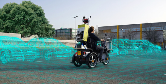
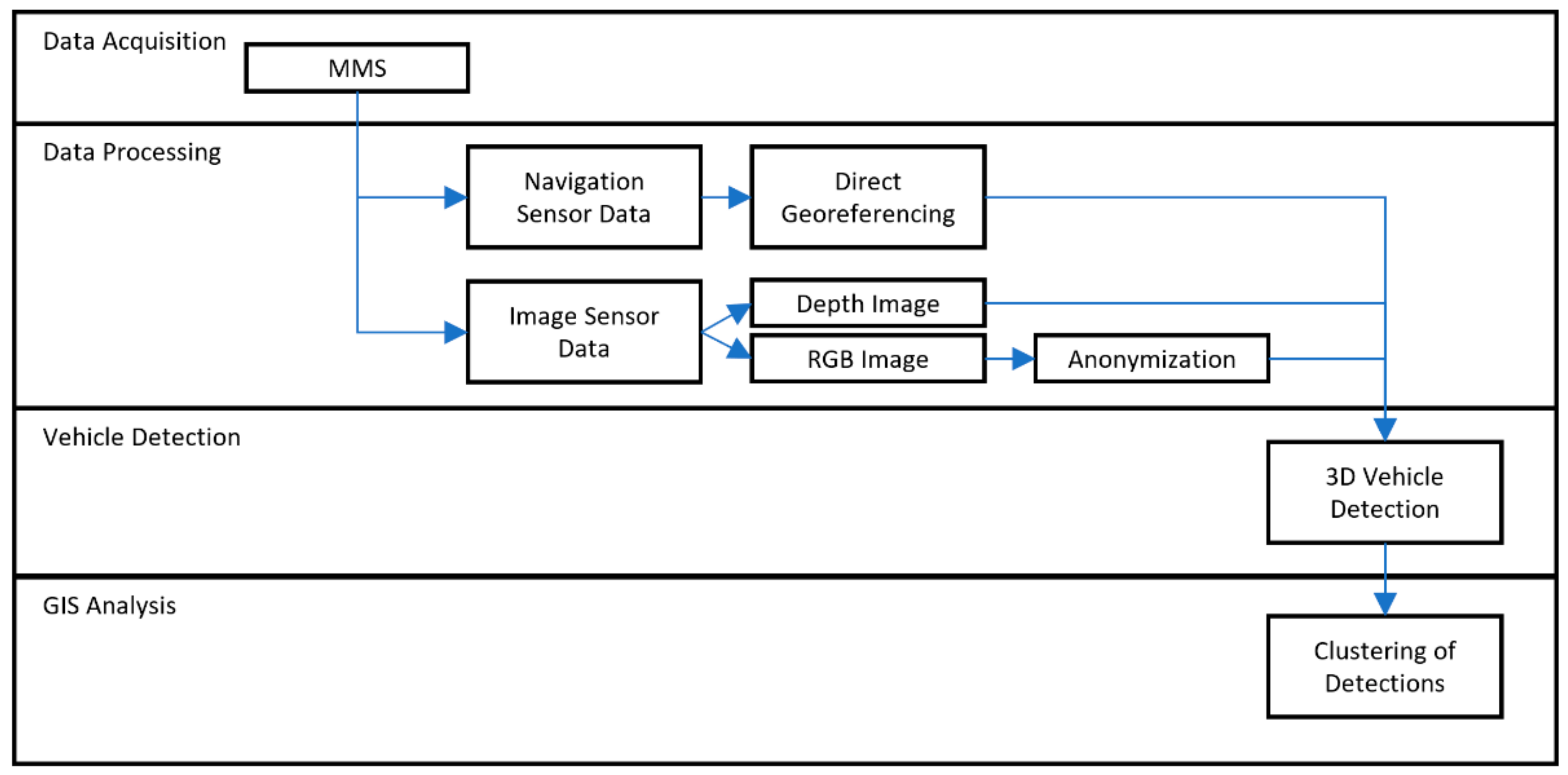
3.1. Overview of System and Workflow

In the following sections, we introduce our mobile mapping platform and payload incorporating two low-cost 3D cameras and a low- to mid-range GNSS/INS system. This is followed by the description of the workflow for deriving on-street parking statistics from georeferenced 3D imagery. The main components of this workflow are illustrated in Figure 1.

3.2. Data Capturing System

For our investigations, we developed a prototypic RGB-D image-based mobile mapping (MM) sensor payload using low-cost components. This enables easy industrialization and scaling of the system in the future. At the present stage of development, we used an electric tricycle as an MM platform. It includes two racks in the front and rear (Figure 2a) where our sensor payloads can be easily attached.

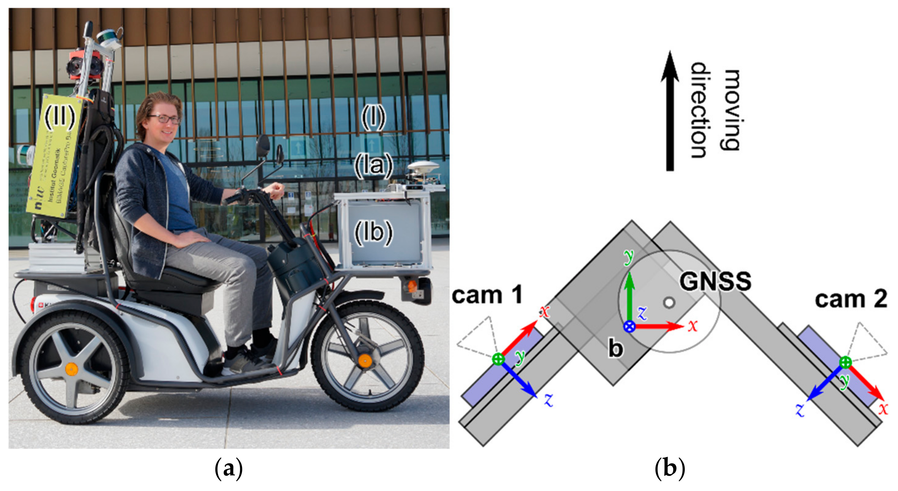
3.2.1. System Components

Our developed MM payload includes both navigation and mapping sensors as well as a computer for data pre-processing and data storage. The GNSS and IMU-based navigation unit SwiftNav Piksi Multi consists of a multi-band and multi-constellation GNSS RTK receiver board and a geodetic GNSS antenna. The GNSS receiver board also includes the consumer-grade IMU Bosch BMI160. Furthermore, the navigation unit provides numerous interfaces, e.g., for external precise hardware-based timestamp creation [39].

For mapping, we used the RGB-D camera Intel RealSense D455. The manufacturer specifies an active stereo depth resolution up to 1280 × 720 pixels and a depth diagonal field of view over 90° (see

Table 1. Sensor specifications of the Intel RealSense D455 [40].

	RGB Sensors	Depth Sensors
Shutter Type	Global Shutter	Global Shutter
Image Sensor	OV9782	OV9282
Max Framerate	90 fps (with max resolution 30 fps)	90 fps (with max resolution 30 fps)
Resolution	1 MP (1280 × 800 px/3 µm)	1 MP (1280 × 720 px/3 µm)
Field of View	H:87° ± 3/V:58° ± 1/D:95° ± 3	H:87° ± 3/V:58° ± 1/D:95° ± 3

). Both depth and RGB cameras use a global shutter. The specified depth sensor range is from 0.4 m to over 10 m, but the range can vary depending on the lighting conditions [40]. In addition, the RGB-D camera supports precise hardware-based triggering using electric pulses, which is crucial for kinematic applications. However, external hardware-based triggering is currently only provided for depth images.

Finally, our MM payload includes the embedded single-board computer nVidia Jetson TX2, which includes a powerful nVidia Pascal-family GPU with 256 cuda cores that enables AI-based edge computing with low energy consumption [41].

3.2.2. System Configuration

Our MM sensor payload consists of a robust aluminum frame to which we stably attached our sensor components. We mounted our sensor frame on the front rack of the electrical tricycle. Both navigation and mapping sensors sit on top of the sensor frame (Figure 2a(Ia)), while the computer and the electronics for power supply and sensor synchronization are in the gray box below the sensors (Figure 2a(Ib)).

The aluminum profiles for the sensor configuration on top of the sensor frame are each angled 45° to the corresponding side. We fixed two RGB-D Intel RealSense cameras on it, so that the first camera, cam 1, points to the front left and the second camera, cam 2, points to the front right (Figure 2b). The second camera thus will detect parking spaces and vehicles that are often located on the right-hand side of the road in urban areas. In the case of one-way streets, the first camera will also detect parking spaces on the left side of the road. Furthermore, the oblique mounting ensures common image features in successive image epochs in moving direction.

We mounted the GNSS and IMU-based navigation unit SwiftNav Piksi Multi on top of the sensor configuration, so that the GNSS antenna is as far up and as far forward as possible and does not obscure the field of view of the cameras or the driver’s field of view. At the same time, the GNSS signal should be obscured as little as possible by the driver or by other objects.

In addition, we mounted our self-developed BIMAGE backpack mobile mapping system (MMS) [42,43] on the rear rack of the electrical tricycle. The BIMAGE backpack is a portable high-performance mobile mapping system, which we used in this project as a reference system for our performance investigations.

3.2.3. System Software

For this stage of development, we designed the system software for data capturing as well as for raw data registration. However, our software has a modular and flexible design and is based on the graph-based robotic framework Robot Operating System (ROS) [44]. This forms an ideal basis for further development steps towards edge computing and on-board AI detection. Furthermore, the ROS framework is easily adoptable and expandable in terms of how to integrate new sensors.

We use the ROS Wrapper for Intel RealSense Devices [45], which is provided and maintained by Intel for the RealSense camera control. For hardware-based device triggering, we use our self-developed ROS trigger node.

3.2.4. Data Acquisition and Georeferencing

Generally, an MM campaign using GNSS/INS-based direct georeferencing starts and ends with the system initialization. The initialization process determines initial position, speed, and rotation values for the Kalman filter used for the state estimation, whereby the azimuth component between the local body frame and the global navigation coordinate frame is the most critical component. The initialization requires a dynamic phase, which from experience requires about three minutes with good GNSS coverage. The initialization procedure at the beginning and at the end of a campaign enables combined forward as well as backward trajectory post-processing, thus ensuring an optimal trajectory estimation.

During the campaign, the computer triggers both RealSense RGB-D cameras as well as the navigation unit with 5 fps. The navigation unit generates precise timestamps of the camera triggering and continuously registers GNSS and IMU raw data on a local SD card. At the same time, the computer receives both RGB and depth image raw data, which are stored in a so-called ROS bag file on an external solid-state drive (SSD).

A first post-processing workflow converts the image raw data into RGB-D images and performs a combined tightly coupled forward and backward GNSS and IMU sensor data fusion and trajectory processing in Waypoint Inertial Explorer [46]. By interpolating the precise trigger timestamps, each RGB-D image finally receives an associated directly georeferenced pose.

3.3. Data Pre-Processing

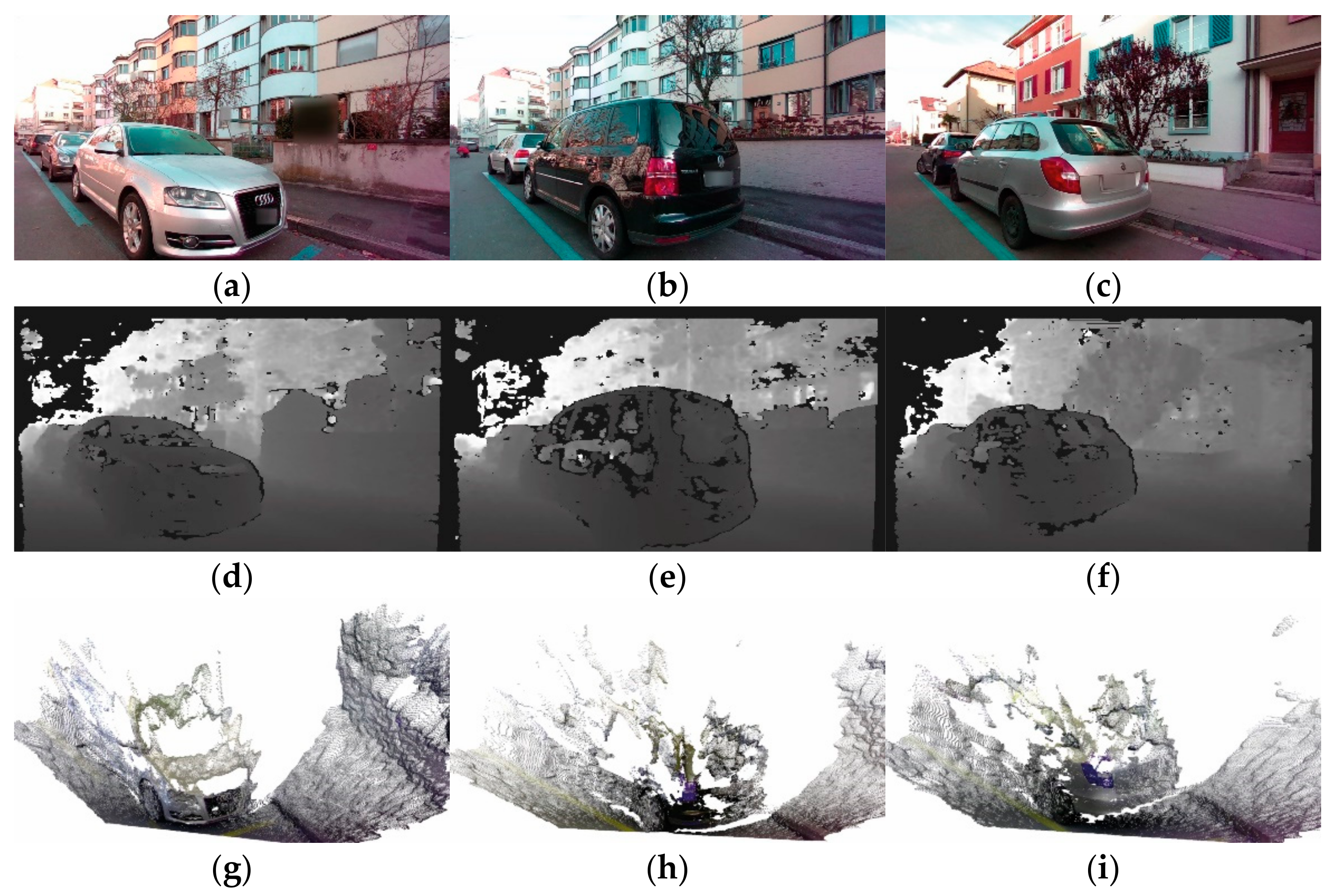
3.3.1. Data Anonymization

Anonymization of the image data was a critical issue for the City of Basel as a project partner. Therefore, the anonymization workflow was developed in close cooperation with the state data protection officer and verified by the same at the end. The open-source software “Anonymizer” [47] is used to anonymize personal image data in the street environment. The anonymization process of images is divided into two steps. First, faces and vehicle license plates are detected in the input images by a neural network pre-trained on a non-open dataset [47]. In the second step, the detected objects are blurred by a Gaussian filter and an anonymized version of the input image is saved. In “Anonymizer”, both the probability scores of the detected objects and the intensity of the blurring can be chosen. The parameters used were selected empirically, whereby a good compromise had to be found between reliable anonymization and as few unnecessarily obscured areas in the images as possible.

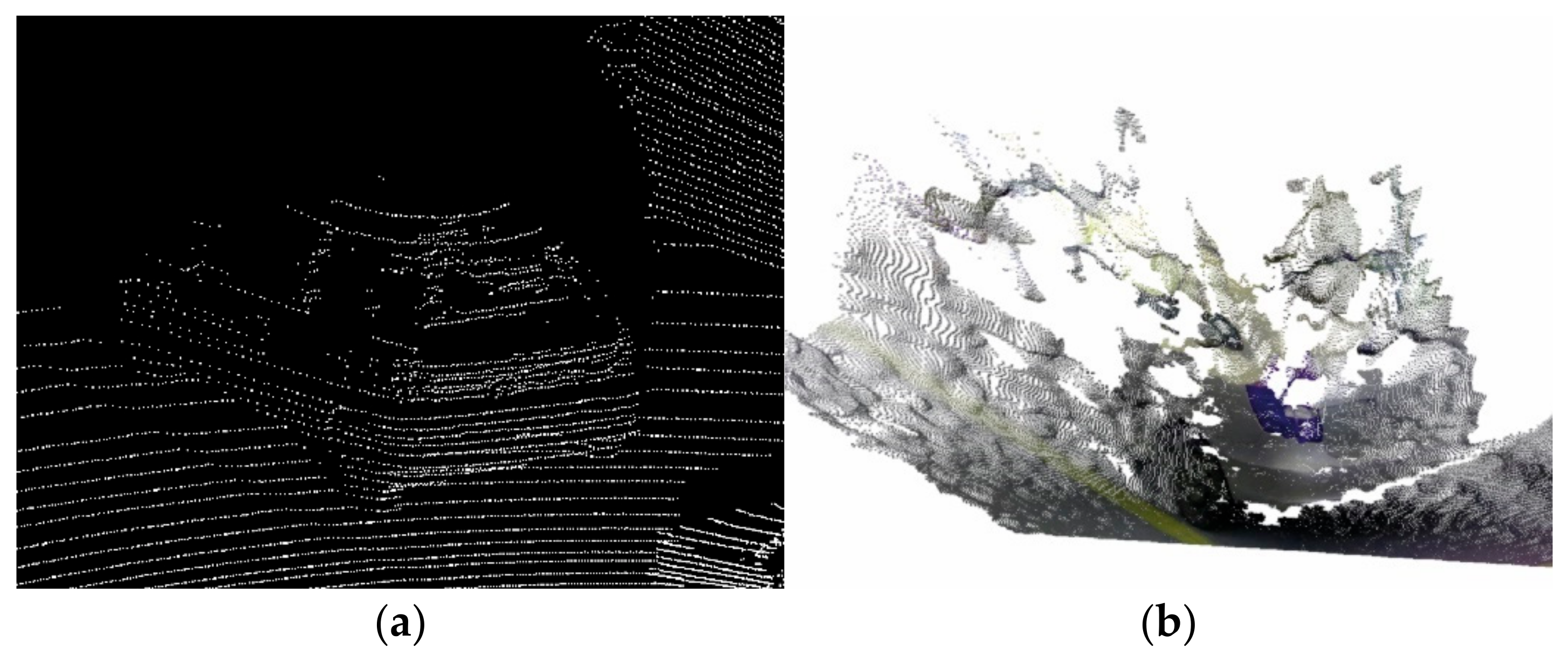
3.3.2. Conversion of Depth Maps to Point Clouds

All vehicle detection algorithms tested and used in this project require point clouds as input data. As point clouds are not directly stored in our system configuration, an additional pre-processing step is necessary. In this step, the point clouds are computed using the geometric relationships between camera geometry and depth maps. The resulting point clouds are cropped to a range of 0.4–8 m, because noise increases strongly beyond this range (see experiments and results in Section 4.3) and are saved as binary files. Figure 3 shows three typical urban scenes with parked cars in the top row, the corresponding depth maps in the middle row, and perspective views of the resulting point clouds in the bottom row. The depth maps in the middle row show some significant data gaps, especially in areas with very high reflectance, which are typical for shiny car bodies (in particular, Figure 3e). The bottom row illustrates the relatively high noise level in the point clouds, which results from the low-cost 3D cameras.

3.4. 3D Vehicle Detection and Mapping

3.4.1. AI-Based 3D Detection

The detection of other road users and vehicles in traffic is an important aspect in the field of autonomous driving. To solve the problem of accurate and reliable 3D vehicle detections, there are a variety of approaches. A good overview of the available approaches and their performance is provided by the leaderboard of the KITTI 3D object detection benchmark [33]. Because the best approaches on the leaderboard are all based on point clouds, only those were considered in this project. At the time of the investigations, the best approach was PV-RCNN [32]. In the freely available open-source project OpenPCDet [48], besides the official implementation of PV-RCNN, other point cloud-based approaches for 3D object detection are provided. These are:

• PointPillars [49]
• SECOND [50]
• PointRCNN [31]
• Part-A2 net [51]
• PV-RCNN [32].

All the approaches listed above were trained using the point clouds from the KITTI 3D object detection benchmark [52]. It should be noted that only point clouds of the classes car, pedestrian, and cyclist were used for the training. The KITTI point clouds were acquired with a high-end Velodyne HDL-64E LiDAR scanner mounted on a car about 1.8 m above the ground [52]. Figure 4 shows a comparison between the point clouds provided in the KITTI benchmark and our own point clouds acquired with the RealSense D455. The KITTI point clouds are sparse, and the edges of the vehicles are clearly visible (Figure 4a). By contrast, our point clouds are much denser, but edges cannot really be detected (Figure 4b). In addition, our point clouds also have significantly higher noise. This can be seen very well on surfaces that should be even, such as the road surface or the sides of the vehicle.

Due to the higher noise in our own point clouds and the lower mounting of the sensor by about half a meter compared with the KITTI benchmark, the question arose as to whether the models pre-trained with the KITTI datasets could be successfully applied to our data. For this purpose, all approaches provided in OpenPCDet were evaluated in a small test area with 32 parked cars and 2 parked vans (Figure 5). PointRCNN [31] detected 32 out of 34 vehicles correctly and did not provide any false detections. In contrast, all other approaches could only detect very few vehicles correctly (13 or less out of 34). Based on these results, we decided to use the method PointRCNN for 3D vehicle detection, which consists of two stages. In stage 1, 3D proposals are generated directly from the raw point cloud in a bottom-up manner via segmenting the point cloud of the whole scene into foreground points and background. In the second stage, the proposals are refined in the canonical coordinates to obtain the final detection results [31].

Parking space management in geographic information systems (GIS) relies on two-dimensional data in a geodetic reference frame, further referred to as world coordinates. Therefore, the detected 3D bounding boxes must be transformed from local sensor coordinates to world coordinates, converted into 2D bounding boxes, and exported in an appropriate format. For this purpose, the OpenPCDet software has been extended to include these aspects. The transformation to world coordinates is performed by applying the sensor poses from direct georeferencing as transformation. The conversion from 3D to 2D bounding boxes is done by projecting the base plane of the 3D bounding box onto the xy-plane by omitting the z coordinates. The resulting 2D bounding boxes as well as the associated class labels and the probability scores of the detected vehicles are exported in GeoJSON format [53] for further processing. The availability of co-registered RGB imagery and depth data resulting from the use of RGB-D sensors has several advantages: it allows the visual verification of the detection results in the imagery, e.g., as part of the feedback loop of a future production system. The co-registered imagery could also be used to facilitate future retraining of existing vehicle classes or for the training of new, currently unsupported vehicle classes.

3.4.2. GIS Analysis

Following the object detection, we currently employ a GIS analysis in QGIS [54] to obtain the number of parked vehicles from the detection results. Since the vehicle detection algorithm returns all detection results, the highly redundant 2D bounding boxes must first be filtered based on their probability scores. For the parking statistics, we only use detected vehicles with a score greater than 0.9 (90% probability). For each vehicle, several 2D-bounding boxes remain after filtering (Figure 6); hence, we perform clustering.

First, each of the filtered 2D bounding boxes is assigned a unique ID and its centroid is calculated. Then the centroids are clustered using the density-based DBSCAN algorithm [55]. Each centroid point is checked as to whether it has a minimum number of neighboring points (minPts) within a radius (ε). Based on this classification, the clusters are formed. The parameters ε and minPts were chosen as 0.5 m and 3, respectively. The bounding boxes are linked to the DBSCAN classes, a minimal bounding box is determined for each cluster class, and the centroid of the new bounding box is calculated. To obtain the number of parked vehicles, the points (centroids of minimal bounding boxes of clusters) within the parking polygons are counted (Figure 7). In combination with the known number of parking spaces per polygon, it is straightforward to create statistics on the occupancy of parking spaces.

Since we count the centroids of clustered vehicle detections within the parking spaces, moving vehicles on the streets do not influence the result. Hence, we do not need to perform a removal of moving vehicles, such as in Bock et al. [4]. Furthermore, we assume that while the parked cars are recorded, they are static. Among other things, this assumption can also be made because the passing MM vehicle prevents other vehicles from leaving or entering parking spaces during capturing.

4. Experiments and Results

Our proposed low-cost MMS and object detection approach consists of three main components determining the capabilities and performance of the overall system: the low-cost navigation unit, the low-cost 3D cameras, and the AI-based object detection algorithms. This section contains a short introduction to the study areas and the test data (Figure 8), followed by a description of the three main experiments aimed at evaluating the main components and the overall system performance:

• Georeferencing investigations in demanding urban environments
• 3D camera performance evaluation in indoor and outdoor settings
• AI-based 3D vehicle detection experiments in a representative urban environment with different parking types.

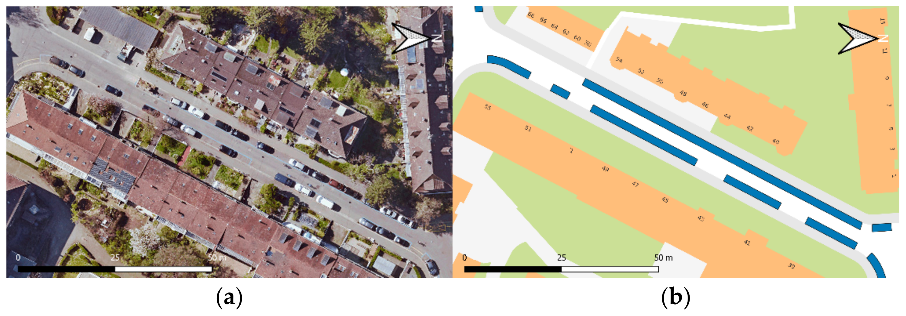
4.1. Study Areas and Data

Our proposed system was evaluated using datasets from two mobile mapping campaigns in demanding urban and suburban environments (see Figure 8 and

Table 2. Overview of two mobile mapping campaigns with their main purpose, characteristics, and the resulting datasets.

Test Campaign Characteristics	Basel City	Muttenz
Main purpose	Evaluation of 3D vehicle detection for different on-street parking types	Georeferencing investigations with parallel operation of the low-cost MMS and a high-end reference MMS
Payload/Sensors	Front: Low-cost MM payload with single RealSense D455	Front: Low-cost MM payload with dual RealSense D455 Back: High-end BIMAGE Backpack as a reference system (for configuration, see Figure 2a)
Characteristics of test area	Residential district, west of the city center of Basel; roads often lined by multi-story buildings and trees; route mostly flat, selected to encompass a large variety of parking slot types	Suburban town located southeast of Basel; route passing shopping district and historical center; route partially lined by large trees; partially steep roads and large elevation differences
Acquisition date	11 December 2020	3 April 2021
Trajectory length	9.7 km	3.4 km
Average acquisition speed	9 km/h	10 km/h
GNSS epochs	~3500	~3500
Image capturing frame rates	5 fps (D455)	5 fps (D455)/1 fps (BIMAGE)
Number of RGB-D images	22,382	5443

). The test areas are representative of typical European cities and suburbs in terms of building heights, streets widths, vegetation/trees, and a variety of on-street parking types.

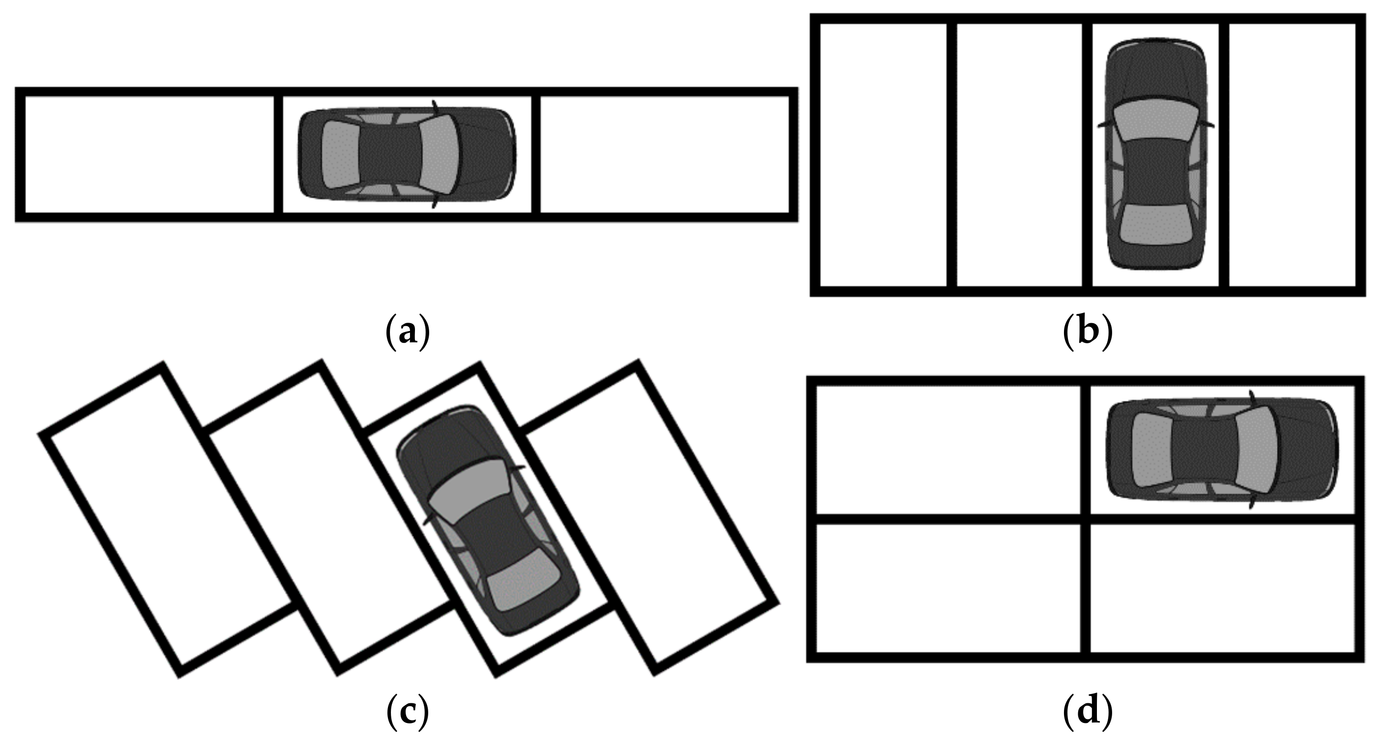
Investigated On-Street Parking Types

Four different types of parking slots that can be found along the campaign route “Basel city” were included, as depicted in Figure 8a: parallel, perpendicular, angle, and 2 × 2 block parking. This allowed us to develop and test a workflow capable of handling each type. With each parking type also comes a unique set of challenges to accurately detect parked vehicles. In the case of several densely perpendicularly parked vehicles (Figure 9b), only a small section of the vehicle facing the road is seen by the cameras. Similarly, with angled parking spaces such as that shown in Figure 9c, a large car (e.g., minivan or SUV) can obstruct the view of a considerably smaller vehicle parked in the following space, leading to fewer or no detections. Lastly, one of the residential roads contains a rather unique parking slot type: an arrangement of 2 × 2 parking spaces on one side of the road (Figure 9d). The main challenge with this type of on-street parking is to be able to correctly identify a vehicle parked in the second, more distant row when all four spaces are occupied.

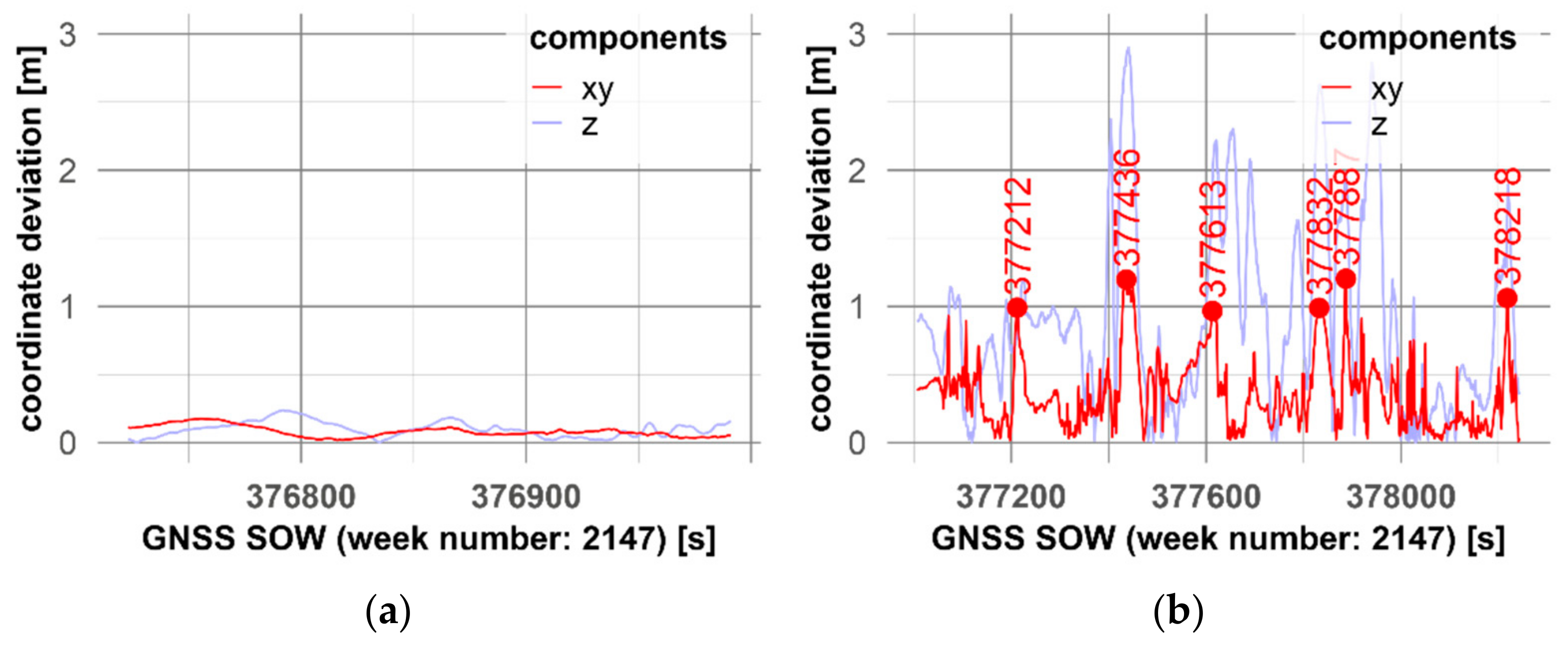
4.2. Georeferencing Investigations

As outlined in Section 3.2.2., a high-end backpack MMS (Figure 2a, II) was installed on the tricycle, serving as a kinematic reference for the low-cost MM payload. In this case, the investigated low-cost system was mounted on the front payload rack of the vehicle and the high-end reference system at the back, resulting in a fixed lever-arm between the two positioning systems. Both systems have independent GNSS and IMU-based navigation sensors. While the sensors of the low-cost MM sensor configuration fall into the consumer grade category, the backpack MMS navigation sensors have tactical grade performance. Since both navigation systems are precisely synchronized using the GNSS time, poses of both systems are accurately time-stamped. Thus, poses from both processed trajectories can be compared, e.g., to estimate the lever arm between both navigation coordinate frames.

$${}^{b_r}T_{b_{lc}}={\left({}^{w}T_{b_r}\right)}^{-1}\ast {}^{w}T_{b_{lc}}$$

(1)

Equation (1) describes the lever arm estimation using transformation matrices for homogeneous coordinates. Here, we consider the poses of the navigation systems as transformations from the respective body frame $b$ to the global navigation coordinate frame $w$. By concatenating the inverse navigation sensor pose of the reference system (backpack MMS) ${}^{w}T_{b_r}$ with the navigation sensor pose of the low-cost MMS ${}^{w}T_{b_{lc}}$, we obtain the transformation ${}^{b_r}T_{b_{lc}}$ from the body frame of the low-cost navigation system $b_{lc}$ to the body frame of the reference (backpack MMS) navigation system $b_r$, from which we extract the lever arm.

To investigate the magnitudes of the position deviations along-track and cross-track, we subtracted the mean lever arm from all estimated lever arm estimations for each acquisition period. Since the georeferencing performance of the high-end BIMAGE backpack—serving as a reference—has been well researched [42,43], we can safely assume that position deviations can be primarily attributed to the investigated low-cost system.

For further 3D vehicle detection and subsequent GIS analysis, an accurate 2D position is crucial. By contrast, the accuracy of the absolute height is negligible due to the back projection onto the 2D xy-plane for the GIS analysis. Therefore, we considered the 2D position and the height separately in the following investigations.

We investigated two different acquisition periods from our dataset from the test site in Muttenz, and we used one pose per second for our examinations. The first “static” period was shortly before moving into the town center, when the system had already initialized but was motionless for 270 s and had good GNSS coverage. By contrast, the second “dynamic” period was from the data acquisition in the village center during 1240 s with various qualities of GNSS reception. For both datasets, we evaluated (a) the intrinsic accuracy provided by the trajectory processing software and (b) the absolute position accuracy, using the high-end system with its estimated pose and the mean lever arm as a reference.

The investigations yielded the following results: In the “static” dataset, the mean intrinsic standard deviation of the estimated 2D positions was 0.6 cm for the reference system and 5.1 cm for the low-cost MM sensor components, respectively. In the “dynamic” dataset, the mean intrinsic standard deviation of the 2D positions was 1.1 cm for the reference system and 10.5 cm for the low-cost MM sensor components, respectively. Regarding the intrinsic standard deviation of the altitudes, they amount to 0.7 cm for the reference system and 7.0 cm for the low-cost MM sensor configuration for the “static” dataset. For the “dynamic” dataset, they amount to 1.1 cm for the reference system and 18.0 cm for the low-cost MM sensor configuration.

The investigations of the absolute coordinate deviations between both trajectories resulted in a mean 2D deviation of 8.3 cm in the “static” dataset and 36.4 cm in the “dynamic dataset”. The mean height deviation amounted to 9.8 cm in the “static” dataset and 90.9 cm in the “dynamic” dataset. The kinematic 2D deviations in the order of 1 m are somewhat larger than the direct georeferencing accuracies of high-end GNSS/IMU systems in challenging urban areas [56].

However, while the coordinate deviations in the “static” dataset remain in a range of approx. 10 cm during the entire period (Figure 10a), they vary strongly in the “dynamic” dataset with 2D position deviation peaks in excess of 100 cm (Figure 10b).

Furthermore, we investigated the environmental conditions of some peaks in Figure 10b to identify possible causes. At second 377,212, only five GNSS satellites were observed, while a building in the southerly direction covers the GNSS reception at second 377,436. At second 377,613, the GNSS reception was affected by dense trees in the easterly direction and at second 377,832 by a church in the south. At second 377,877, a complete loss of satellites occurred, and finally at second 378,218, a tall building in the south interfered with satellite reception.

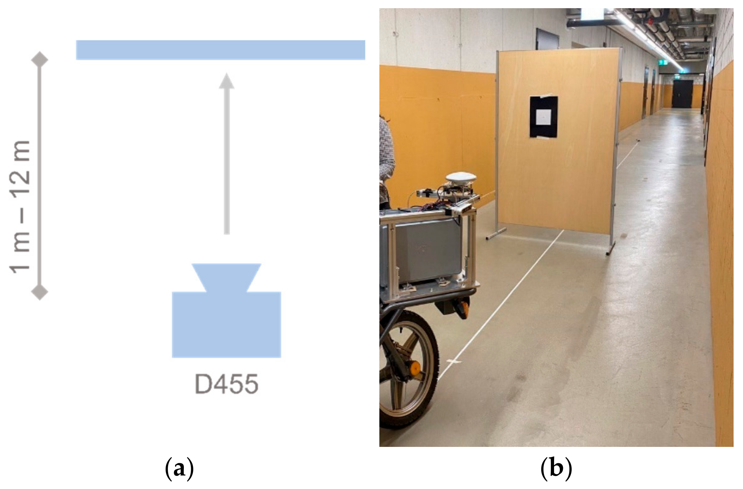
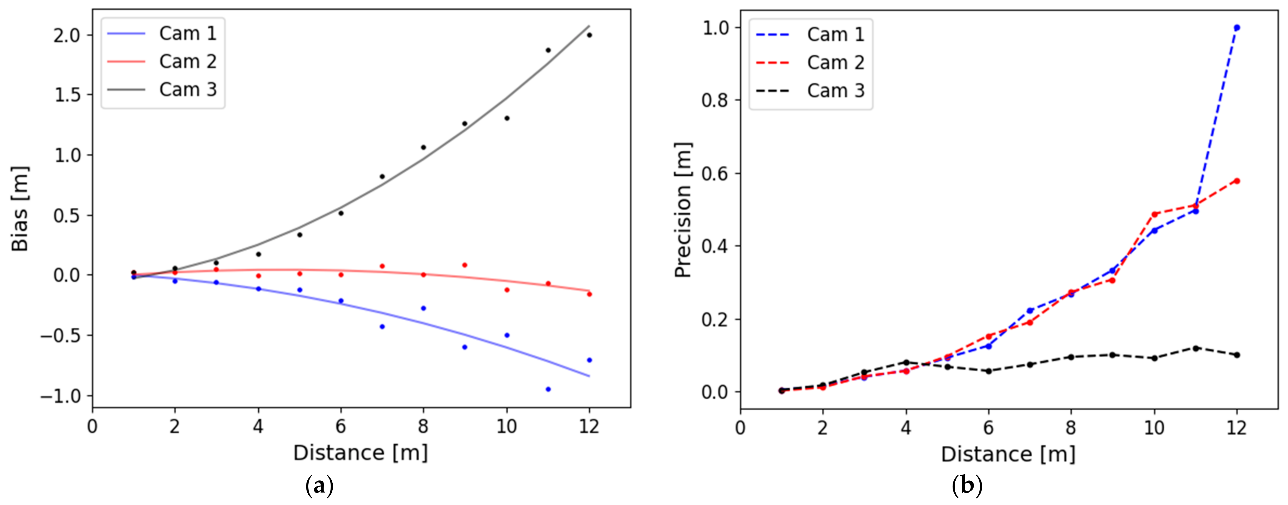
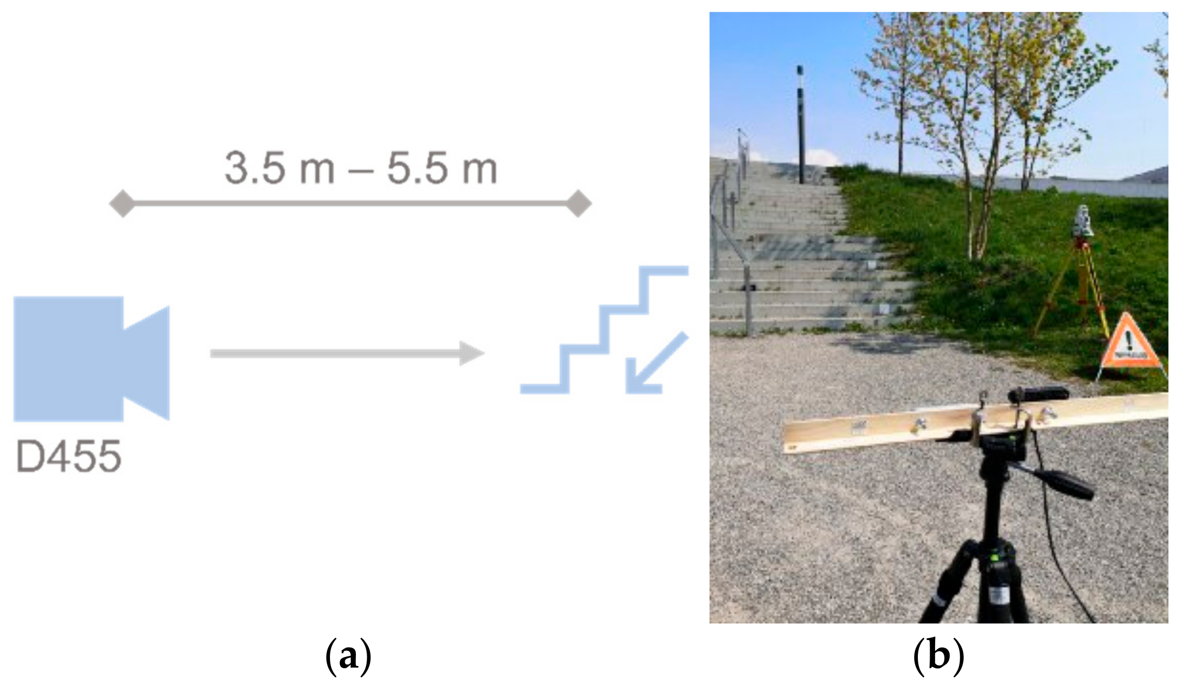
4.3. 3D Camera Performance Evaluation

In earlier investigations by Frey [57], different RealSense 3D camera types, including the solid-state LiDAR model L515 and the active stereo-based models D435 and D455, were compared in indoor and outdoor environments. All 3D cameras performed reasonably well in indoor environments. However, in outdoor environments and under typical daylight conditions, the maximum range of the L515 LiDAR sensor was limited to 1–2 m and that of the D435 to 2–3 m. The latest model D455, however, showed a clearly superior performance in outdoor environments with maximum ranges of more than 5–7 m [57]. Based on these earlier trials, the D455 was chosen for this project and subsequently evaluated in more detail.

4.3.1. Distance-Dependent Depth Estimation

In a first series of experiments, we evaluated bias and precision of the depth measurements with the Intel RealSense D455 in a controlled indoor environment. The evaluation was conducted in line with the methodology and metrics proposed by Helmetschlager-Funek et al. [25]. We examined three units (cam1, cam2, and cam3). The experimental setup consisted of a fixed 3D camera and a reference plane oriented orthogonally to the main viewing direction (Figure 11a,b). This plane was re-positioned in one-meter intervals at measuring distances from 1 to 12 m, leading to a total of 12 evaluated distances. At each interval, 100 frames were captured to obtain a sufficiently large number of measuring samples. Ground-truth measurements were obtained with a measuring tape with an accuracy of approx. 1 cm. The analyses were performed on a 20 × 20 pixel window, and we calculated the average difference to the reference distance (bias) and the precision (standard deviation) over the 100 frames per position.

Table 3. Bias and precision values of depth measurements at 4 m and 8 m with three different RealsSense D455 units with respective colors as shown in Figure 12. Percentage values show the respective metric bias and precision values in relation to the respective range.

	Cam 1 (Blue)		Cam 2 (Red)		Cam 3 (Black)
	Bias	Precision	Bias	Precision	Bias	Precision
4 m	−11 cm (2.8%)	5.7 cm (1.4%)	−1 cm (0.3%)	5.6 cm (1.4%)	17 cm (4.3%)	8.0 cm (2.0%)
8 m	−27 cm (3.4%)	26.8 cm (3.4%)	0 cm (0.0%)	27.2 cm (3.4%)	106 cm (13.3%)	9.4 cm (1.2%)

shows the resulting bias and precision values of the three camera units (cam 1–3) at selected distances of 4 m and 8 m. According to the manufacturer specifications, the D455 should have a depth accuracy (bias) of ≤2% and a standard deviation (precision) of ≤2% for ranges up to 4 m. In our experiments, only cam 2 showed a bias well within the specifications, while the bias of cam 3 was more than double the expected value.

Figure 12a,b show the bias and precision values for all the evaluated measuring distances from 1 to 12 m. Bias and precision show a roughly linear behavior for distances up to 4 (to max. 6 m). For longer ranges, all cameras exhibited a non-linear distance-dependent bias and precision—except cam 3 with an exceptional, nearly constant value for precision. The exponential behavior of the precision can be expected from a stereo system with a small baseline of only 95 mm and a very small b/h ratio for longer measuring distances. The large bias of cam 3 over 4 m and the exponential behavior of its distance-dependent bias values indicate a calibration problem.

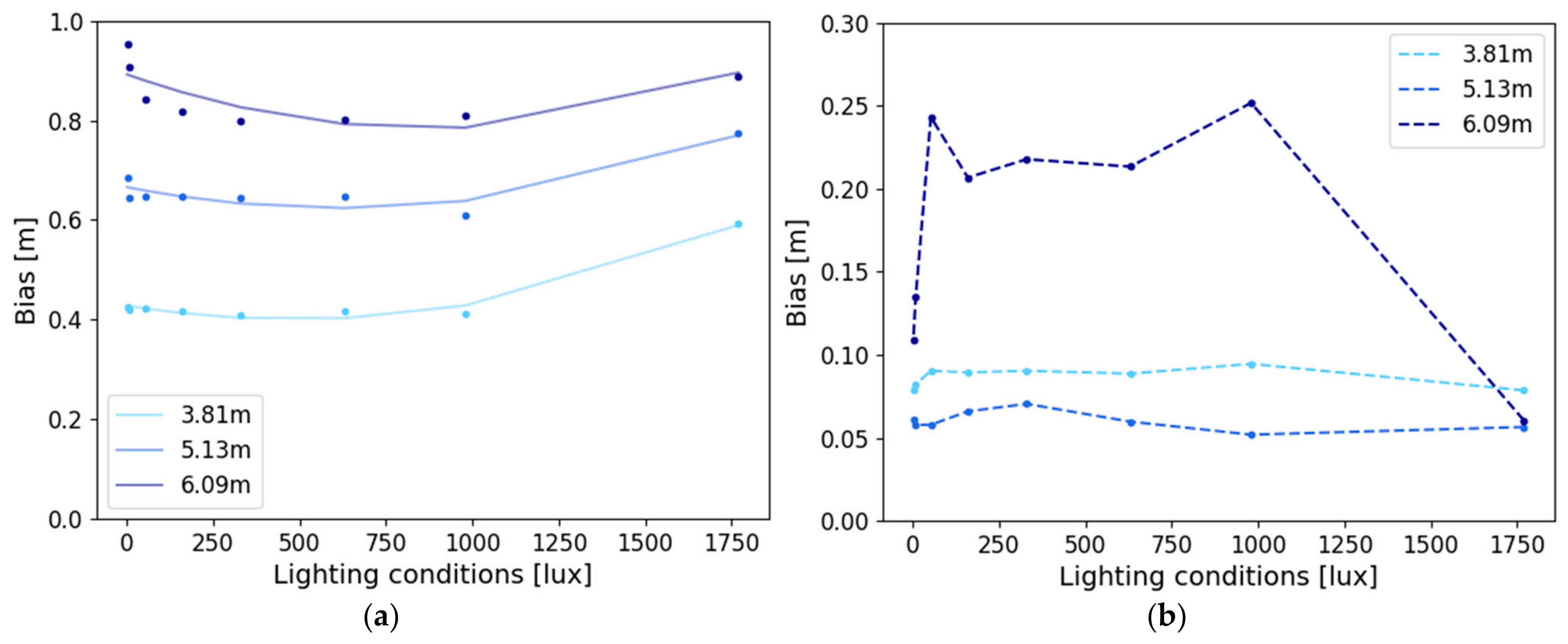
4.3.2. Influence of Lighting Conditions on Outdoor Measurements

Outdoor environments pose several challenges for (3D) cameras, including large variations in lighting conditions and in the radiometric properties of objects to be mapped. The main question of interest was whether the D455 cameras could be operated in full daylight, at dusk, or even at night with only artificial street lighting available. For this purpose, we investigated the influence of lighting conditions on the camera performance.

In this experiment, cam 3 was placed in front of a staircase in the park of the FHNW Campus in Muttenz (Figure 13). Selected steps of the stair featured targets so that three different distances (3.81 m, 5.13 m, 6.09 m) could be evaluated. Additionally, a luxmeter was used for measuring light intensity and a tachymeter for reference distance measurements. The experiment was performed in full daylight on a sunny day with a maximum light intensity of 1770 lux and during sunset until dusk with a minimal intensity of only 2 lux. For comparison, typical indoor office lighting has an intensity of approx. 500 lux.

Data capturing and analysis were carried out in analogy to the indoor experiments outlined above, but this time with the capture of 100 frames per lighting condition and with the evaluation of 20 × 20 pixel windows. Bias values for the three targets were derived by comparing the observed average distance with the respective reference distance.

The results for bias and precision under different lighting conditions are shown in Figure 14a,b. It can be seen in Figure 14a that the bias values for cam 3 exhibit the same distance-based scale effect as already shown in the indoor tests above. Bias and precision values proved to be relatively stable under medium light intensities between 330 and 1000 lux. Slight increases in bias can be observed in very dark and very bright conditions—with a sharp increase for the target at 6.09 m under 1750 lux, for which we currently have no plausible explanation. The highest bias of 0.95 m is with 2 lux at a distance of 6.09 m. This corresponds to the end of the sunset in almost complete darkness. The precision values for the two shorter distances were very stable and consistently below 10 cm, varying only by ±2.4 cm across all investigated illuminations. So, rather surprisingly, lighting conditions seem to have no significant influence on measuring precision. The larger values and variations in precision at a distance of 6.09 m are likely caused by the fact that this target was brown while the others were white.

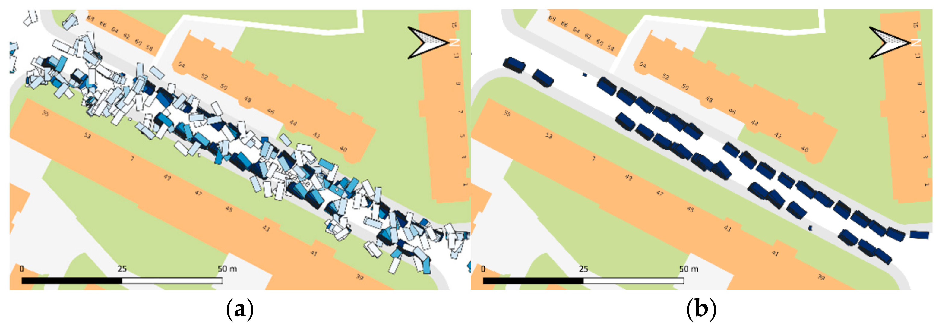
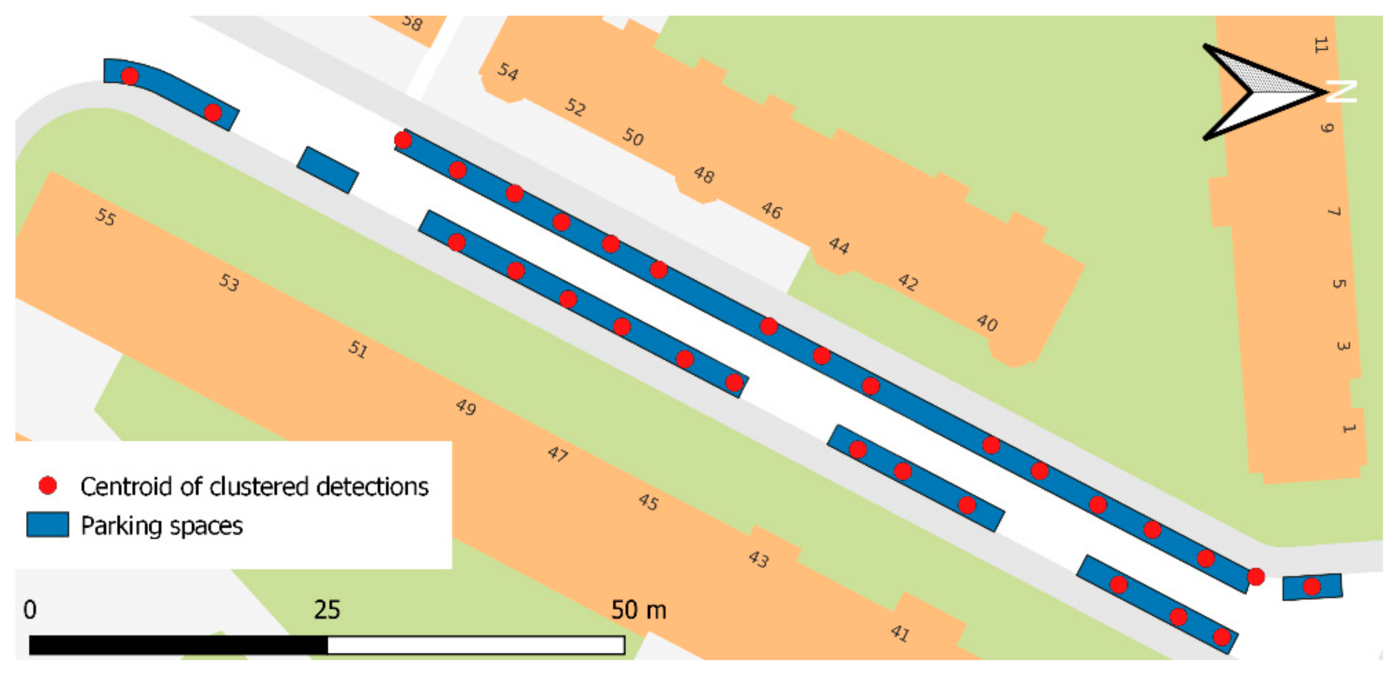
4.4. AI-Based 3D Vehicle Detection

To evaluate the AI-based 3D vehicle detection algorithm used, images of seven streets in the test area Basel were processed according to the workflow described in Section 3.4. The streets were selected so that all parking types were represented. However, since the types of parking spaces occur with different frequencies, their number in the evaluation varies greatly. In total, the selected test streets include 350 parking spaces, of which 283 were occupied. The vehicle detections were manually counted and verified.

Initial investigations using the point cloud-based PointRCNN 3D object detector as part of OpenPCDet yielded a recall of 0.87, whereby no tall vehicles such as family vans, camper vans, or delivery vans were detected. Further investigations revealed that the pre-trained networks provided in OpenPCDet can only detect the classes car, pedestrian, and cyclist and do not yet include classes such as van, truck, or bus. In order to correctly assess the detection capabilities for a vehicle class with existing training data, subsequently only the class “car” representing standard cars (including hatchbacks, sedans, station wagons, etc.) was considered. Thus, all 37 tall vehicles were removed from the dataset. For the evaluation, a total of 313 parking spaces were considered, 246 of which were occupied by cars. Our 3D detection approach achieved an average precision of 1.0 (100%) and an average recall of 0.97 (97%) for all parking types (

Table 4. AI-based detection results for cars, broken down by type of parking space.

	Parallel	Perpendicular	Angle	2 × 2	Overall
True positive	163	49	24	3	239
True negative	36	26	4	1	67
False positive	0	0	0	0	0
False negative	0	3	1	3	7
Precision	1.00	1.00	1.00	1.00	1.00
Recall	1.00	0.94	0.96	0.50	0.97

). Parallel parking showed the best detection rate with a recall of 1.0, followed by angle parking with 0.96 and perpendicular parking with 0.94. Cars parked in 2 × 2 parking slots were significantly harder to detect, resulting in a recall of only 0.50. However, the sample for this type is too small for a statistically sound evaluation.

5. Discussion

5.1. Georeferencing Investigations

Creating valid on-street parking statistics requires absolute object localization accuracies roughly at the meter level if the occupation of individual parking slots is to be correctly determined. As shown in several studies [42,56], georeferencing in urban areas is very challenging, even with high-end MMS. In our georeferencing investigations, we equipped our electrical tricycle with our low-cost mobile mapping payload and with the well-researched high-performance BIMAGE backpack as the second payload, which subsequently served as a reference for static and kinematic experiments. By estimating a lever arm between both systems for each measurement epoch and comparing these estimates with the lever arm fixed to the MMS body frame, the georeferencing performance could successfully be evaluated. The direct georeferencing comparisons yielded a good average 2D deviation between the low-cost and the reference system for the static case of approx. 10 cm. The kinematic tests resulted in an average 2D deviation of 0.9 m, however with peaks of more than 1 m. These peaks can be attributed to locations with extended GNSS signal obstructions caused by buildings or large trees. The georeferencing tests showed that the current low-cost system fulfills the sub-meter accuracy requirements in areas with few to no GNSS obstructions. However, in demanding urban environments it does not yet fulfill these strict requirements, mainly due to its low-quality IMU, and complementary positioning strategies will likely be required. Future research could include the evaluation of higher-grade and possibly redundant low-cost IMUs, and the development of novel map matching approaches offered by 3D cameras. However, the current system shortcomings only limit the absolute localization and automated mapping capabilities of the system; they do not affect the 3D vehicle detection performance and the object clustering, which mainly rely on relative accuracies.

5.2. 3D Camera Performance

In our experiments, we investigated the depth accuracy and precision of RealSense D455 low-cost 3D cameras. In a previous evaluation, this camera type had proven to be the first 3D camera suitable for outdoor applications supporting measuring ranges beyond 4 m. In a first experiment, we investigated three units for depth accuracy (bias) and depth precision (standard deviation) at different measuring distances, ranging from 1 to 12 m. Two of the three units exhibited a depth accuracy and a depth precision with a significant non-linear dependency on measuring range, which confirmed the findings of Halmetschlager et al. [25]. The manufacturer specification [40] of ≤2% accuracy for ranges up to 4 m was only met by one unit. The specification of ≤2% precision was met by all units. The investigations showed that 3D cameras should be tested—and if necessary re-calibrated—if they are to be used for long-range measurements. By limiting the depth measurements to a max. range of 8 m, we limited the localization error contribution of the depth bias to max. 0.3–0.4 m. The second experiment demonstrated that ambient lighting conditions have no significant effect on the depth bias and precision of the RealSense D455—with only a minor degradation in very dark and very bright conditions. This robustness towards different lighting conditions and the capability to reliably operate in very dark and very bright environments is an important factor for our application.

5.3. 3D Object Detection Evaluation

In the last experiment, we addressed the challenge of reliably detecting and localizing vehicles in the point clouds derived from the low-cost 3D cameras, which are significantly noisier and have more data gaps than LiDAR-based point clouds. In an evaluation of five candidate 3D object detection algorithms, PointRCNN clearly outperformed all the others. On our dataset in the city of Basel with four different parking types (parallel, perpendicular, angle, and 2 × 2 blocks) and a total of 313 parking spaces, we obtained an average precision of 100% and an initial average recall of 97%. These detection results apply for the class “car”, representing typical standard cars such as sedans, hatchbacks, etc. It should be noted that our current detection framework has not yet been trained for other vehicle classes such as vans, buses, or trucks. Consequently, tall vehicles such as family or delivery vans are not yet detected. For the supported class of cars, our approach outperformed the other approaches (Mathur et al. [3], Bock et al. [4], Grassi et al. [11], and Fetscher [5]) in precision and was equal or better for recall. When broken down by the type of parking space, all cars in parallel parking spaces were detected with slightly inferior performance for angle and perpendicular parking (see Table 4). In conclusion, PointRCNN, which was originally developed for and trained with point clouds from high-end LiDAR data, can be successfully applied to depth data from low-cost RGB-D cameras. Ongoing and future research includes the training of PointRCNN for additional vehicle classes, in particular “vans”, which according to our preliminary investigations account for about 10% of the vehicles in the test area. The intention is to use the labeled object classes from the KITTI 3D Object detection benchmark [33] and to complement the training data with RGB-D data from mobile mapping missions with our own system.

5.4. Overall Capabilities and Performance

Table 5. Comparison of our method with the main methods for deriving on-street parking statistics from mobile sensors.

	Mathur et al. [3]	Bock et al. [4]	Grassi et al. [11]	Fetscher [5]	Ours
Mapping platform	Probe vehicles (e.g., taxis)	High-end MLS vehicle	Vehicle (dashboard-mounted)	High-end multi-view stereo MMS	Electric Tricycle
Mapping sensors/mapping data	Ultrasonic range finder/range profiles	Dual LiDAR/3D point clouds	Smartphone camera/2D imagery	High-end stereo cameras/RGB-D imagery	Low-cost 3D camera/RGB-D imagery
Revisit frequency	potentially high	on-demand	potentially high	low	potentially high
Supported parking types	parallel only	parallel, perpendicular	parallel only	parallel, angle, perpendicular, 2 × 2 clusters	parallel, angle, perpendicular, 2 × 2 clusters
Detection type	gaps (in range profiles)	object segmentation and classification (RF)	image-based car detection	corner detection or clustering	AI-based 3D object detection (PointRCNN)
Sample size (# of slots or vehicles)	57	717	8176	184	313
Detection accuracy	~90% (of free spaces)	Recall 93.7% Precision 97.4%	~90%	97.0–98.3%	Recall 97% Precision 100%

shows a comparison of our method with the state-of-the-art methods introduced in Section 2. It shows that our low-cost system has the potential for the necessary revisit frequencies, e.g., for temporal parking analyses over the course of the day. The comparison also shows that only our approach and the one by Fetscher [5] support the three main parking types of parallel, angle, and perpendicular parking. However, the latter method by Fetscher is not suitable for practical statistics due to its reliance on street-level imagery. One of the advantages of our approach is the availability of the complementary nature of the co-registered RGB imagery and depth data from the 3D cameras. This not only allows for the visual inspection of the detection results, but it will also facilitate future retraining of existing vehicle classes or the training of new, currently unsupported vehicle classes in 3D object detection, e.g., by exploiting labels from 2D object detection and segmentation [13].

6. Conclusions and Future Work

In this article, we introduced a novel system and approach for creating on-street parking statistics by combining a low-cost mobile mapping payload featuring RGB-D cameras with AI-based 3D vehicle detection algorithms. The new payload integrates two active stereo RGB-D consumer cameras of the latest generation, an entry-level GNSS/INS positioning system, and an embedded single-board computer using the Robot Operating System (ROS). Following direct georeferencing and anonymization steps, the RGB-D imagery is converted to 3D point clouds. These are subsequently used by PointRCNN for detecting vehicle location, size, and orientation—subsequently represented by 3D bounding boxes. These vehicle detection candidates and their scores are subsequently used for a GIS-based creation of parking statistics. The new automated mobile mapping and 3D vehicle detection approach yielded a precision of 100% and an average recall of 97% for cars and can support all common parking types, including perpendicular and angle parking. To our knowledge, this is one of the first studies successfully using low-cost 3D cameras for kinematic mapping purposes in an outdoor environment.

In our study, we investigated several critical components of a mobile mapping solution for automatically detecting parked cars and creating parking statistics, namely, georeferencing accuracy, 3D camera performance, and AI-based vehicle detection.

The methods and results described in this paper leave room for further improvement. One of the first goals is the training of the PointRCNN detector to allow the detection of tall vehicles and vans. For this purpose, a reasonably large training and validation dataset will be collected in further mobile mapping missions. Another goal is to employ edge computing for onboard 3D object detection. This would eliminate the current need for massive onboard data storage performance and capacity, would avoid privacy issues, and would dramatically reduce the post-processing time. Finally, we will investigate novel map matching strategies, which will be offered by the RGB-D data and which will avoid some of the current difficulties with direct georeferencing.

References

1. Shoup, D.C. Cruising for Parking. Transp. Policy 2006, 13, 479–486. [Google Scholar] [CrossRef]
2. Rapp Trans AG Basel-Stadt. Erhebung Parkplatzauslastung Stadt Basel 2019; Version 1; RAPP Group: Basel, Switzerland, 2019. [Google Scholar]
3. Mathur, S.; Jin, T.; Kasturirangan, N.; Chandrasekaran, J.; Xue, W.; Gruteser, M.; Trappe, W. ParkNet. In Proceedings of the 8th International Conference on Mobile Systems, Applications and Services—MobiSys’10, San Francisco, CA, USA, 15–18 June 2010; p. 123. [Google Scholar] [CrossRef]
4. Bock, F.; Eggert, D.; Sester, M. On-Street Parking Statistics Using LiDAR Mobile Mapping. In Proceedings of the 2015 IEEE 18th International Conference on Intelligent Transportation Systems, Gran Canaria, Spain, 15–18 September 2015; pp. 2812–2818. [Google Scholar] [CrossRef]
5. Fetscher, S. Automatische Analyse von Streetlevel-Bilddaten Für das Digitale Parkplatzmanagement. Bachelor’s Thesis, FHNW University of Applied Sciences and Arts Northwestern Switzerland, Muttenz, Switzerland, 2020. [Google Scholar]
6. Polycarpou, E.; Lambrinos, L.; Protopapadakis, E. Smart Parking Solutions for Urban Areas. In Proceedings of the 2013 IEEE 14th International Symposium on “A World of Wireless, Mobile and Multimedia Networks” (WoWMoM), Madrid, Spain, 4–7 June 2013; pp. 1–6. [Google Scholar] [CrossRef]
7. Paidi, V.; Fleyeh, H.; Håkansson, J.; Nyberg, R.G. Smart Parking Sensors, Technologies and Applications for Open Parking Lots: A Review. IET Intell. Transp. Syst. 2018, 12, 735–741. [Google Scholar] [CrossRef]
8. Barriga, J.J.; Sulca, J.; León, J.L.; Ulloa, A.; Portero, D.; Andrade, R.; Yoo, S.G. Smart Parking: A Literature Review from the Technological Perspective. Appl. Sci. 2019, 9, 4569. [Google Scholar] [CrossRef] [Green Version]
9. Houben, S.; Komar, M.; Hohm, A.; Luke, S.; Neuhausen, M.; Schlipsing, M. On-Vehicle Video-Based Parking Lot Recognition with Fisheye Optics. In Proceedings of the 16th International IEEE Conference on Intelligent Transportation Systems (ITSC 2013), The Hague, The Netherlands, 6–9 October 2013; pp. 7–12. [Google Scholar] [CrossRef]
10. Suhr, J.; Jung, H. A Universal Vacant Parking Slot Recognition System Using Sensors Mounted on Off-the-Shelf Vehicles. Sensors 2018, 18, 1213. [Google Scholar] [CrossRef] [Green Version]
11. Grassi, G.; Jamieson, K.; Bahl, P.; Pau, G. Parkmaster: An in–Vehicle, Edge–Based Video Analytics Service for Detecting Open Parking Spaces in Urban Environments. In Proceedings of the Second ACM/IEEE Symposium on Edge Computing, San Jose, CA, USA, 12–14 October 2017; pp. 1–14. [Google Scholar] [CrossRef] [Green Version]
12. Nebiker, S.; Cavegn, S.; Loesch, B. Cloud-Based Geospatial 3D Image Spaces—A Powerful Urban Model for the Smart City. ISPRS Int. J. Geo-Inf. 2015, 4, 2267–2291. [Google Scholar] [CrossRef] [Green Version]
13. Wu, Y.; Kirillov, A.; Massa, F.; Lo, W.-Y.; Girshick, R. Detectron2. 2019. Available online: https://github.com/facebookresearch/detectron2 (accessed on 3 August 2021).
14. Ulrich, L.; Vezzetti, E.; Moos, S.; Marcolin, F. Analysis of RGB-D Camera Technologies for Supporting Different Facial Usage Scenarios. Multimed. Tools Appl. 2020, 79, 29375–29398. [Google Scholar] [CrossRef]
15. Kuznetsova, A.; Leal-Taixe, L.; Rosenhahn, B. Real-Time Sign Language Recognition Using a Consumer Depth Camera. In Proceedings of the 2013 IEEE International Conference on Computer Vision Workshops, Sydney, Australia, 2–8 December 2013; pp. 83–90. [Google Scholar] [CrossRef]
16. Jain, H.P.; Subramanian, A.; Das, S.; Mittal, A. Real-Time Upper-Body Human Pose Estimation Using a Depth Camera. In Proceedings of the International Conference on Computer Vision/Computer Graphics Collaboration Techniques and Applications, Rocquencourt, France, 10–11 October 2011; pp. 227–238. [Google Scholar]
17. Zollhöfer, M.; Stotko, P.; Görlitz, A.; Theobalt, C.; Nießner, M.; Klein, R.; Kolb, A. State of the Art on 3D Reconstruction with RGB-D Cameras. Comput. Graph. Forum 2018, 37, 625–652. [Google Scholar] [CrossRef]
18. Holdener, D.; Nebiker, S.; Blaser, S. Design and Implementation of a Novel Portable 360° Stereo Camera System with Low-Cost Action Cameras. Int. Arch. Photogramm. Remote Sens. Spat. Inf. Sci. 2017, 42, 105–110. [Google Scholar] [CrossRef] [Green Version]
19. Hasler, O.; Blaser, S.; Nebiker, S. Performance evaluation of a mobile mapping application using smartphones and augmented reality frameworks. ISPRS Ann. Photogramm. Remote Sens. Spat. Inf. Sci. 2020, 5, 741–747. [Google Scholar] [CrossRef]
20. Torresani, A.; Menna, F.; Battisti, R.; Remondino, F. A V-SLAM Guided and Portable System for Photogrammetric Applications. Remote Sens. 2021, 13, 2351. [Google Scholar] [CrossRef]
21. Henry, P.; Krainin, M.; Herbst, E.; Ren, X.; Fox, D. RGB-D Mapping: Using Kinect-Style Depth Cameras for Dense 3D Modeling of Indoor Environments. Int. J. Rob. Res. 2012, 31, 647–663. [Google Scholar] [CrossRef] [Green Version]
22. Henry, P.; Krainin, M.; Herbst, E.; Ren, X.; Fox, D. RGB-D Mapping: Using Depth Cameras for Dense 3D Modeling of Indoor Environments. In Experimental Robotics; Springer: Berlin/Heidelberg, Germany, 2014; pp. 477–491. [Google Scholar]
23. Brahmanage, G.; Leung, H. Outdoor RGB-D Mapping Using Intel-RealSense. In Proceedings of the 2019 IEEE SENSORS, Montreal, QC, Canada, 27–30 October 2019; pp. 1–4. [Google Scholar] [CrossRef]
24. Iwaszczuk, D.; Koppanyi, Z.; Pfrang, J.; Toth, C. Evaluation of a mobile multi-sensor system for seamless outdoor and indoor mapping. Int. Arch. Photogramm. Remote Sens. Spat. Inf. Sci. 2019, XLII-1/W2, 31–35. [Google Scholar] [CrossRef]
25. Halmetschlager-Funek, G.; Suchi, M.; Kampel, M.; Vincze, M. An Empirical Evaluation of Ten Depth Cameras: Bias, Precision, Lateral Noise, Different Lighting Conditions and Materials, and Multiple Sensor Setups in Indoor Environments. IEEE Robot. Autom. Mag. 2019, 26, 67–77. [Google Scholar] [CrossRef]
26. Lourenço, F.; Araujo, H. Intel RealSense SR305, D415 and L515: Experimental Evaluation and Comparison of Depth Estimation. In Proceedings of the 16th International Joint Conference on Computer Vision, Imaging and Computer Graphics Theory and Applications (VISIGRAPP 2021), Online Streaming, 8–10 February 2021; Volume 4, pp. 362–369. [Google Scholar] [CrossRef]
27. Vit, A.; Shani, G. Comparing RGB-D Sensors for Close Range Outdoor Agricultural Phenotyping. Sensors 2018, 18, 4413. [Google Scholar] [CrossRef] [Green Version]
28. Zhao, Z.Q.; Zheng, P.; Xu, S.T.; Wu, X. Object Detection with Deep Learning: A Review. IEEE Trans. Neural Netw. Learn. Syst. 2019, 30, 3212–3232. [Google Scholar] [CrossRef] [Green Version]
29. Friederich, J.; Zschech, P. Review and Systematization of Solutions for 3d Object Detection. In Proceedings of the 15th International Conference on Business Information Systems, Potsdam, Germany, 8–11 March 2020. [Google Scholar] [CrossRef]
30. Arnold, E.; Al-Jarrah, O.Y.; Dianati, M.; Fallah, S.; Oxtoby, D.; Mouzakitis, A. A Survey on 3D Object Detection Methods for Autonomous Driving Applications. IEEE Trans. Intell. Transp. Syst. 2019, 20, 3782–3795. [Google Scholar] [CrossRef] [Green Version]
31. Shi, S.; Wang, X.; Li, H. PointRCNN: 3D Object Proposal Generation and Detection from Point Cloud. In Proceedings of the IEEE Computer Society Conference on Computer Vision and Pattern Recognition, Long Beach, CA, USA, 16–20 June 2019; pp. 770–779. [Google Scholar] [CrossRef] [Green Version]
32. Shi, S.; Guo, C.; Jiang, L.; Wang, Z.; Shi, J.; Wang, X.; Li, H. PV-RCNN: Point-Voxel Feature Set Abstraction for 3D Object Detection. In Proceedings of the Conference on Computer Vision and Pattern Recognition, Seattle, WA, USA, 14–19 June 2020; pp. 10526–10535. [Google Scholar] [CrossRef]
33. KITTI 3D Object Detection Online Benchmark. Available online: http://www.cvlibs.net/datasets/kitti/eval_object.php?obj_benchmark=3d (accessed on 29 July 2021).
34. Zheng, W.; Tang, W.; Jiang, L.; Fu, C.-W. SE-SSD: Self-Ensembling Single-Stage Object Detector from Point Cloud. arXiv 2021, arXiv:2104.09804. [Google Scholar]
35. Li, Z.; Yao, Y.; Quan, Z.; Yang, W.; Xie, J. SIENet: Spatial Information Enhancement Network for 3D Object Detection from Point Cloud. arXiv 2021, arXiv:2103.15396. [Google Scholar]
36. Deng, J.; Shi, S.; Li, P.; Zhou, W.; Zhang, Y.; Li, H. Voxel R-CNN: Towards High Performance Voxel-Based 3D Object Detection. arXiv 2020, arXiv:2012.15712. [Google Scholar]
37. Qi, C.R.; Liu, W.; Wu, C.; Su, H.; Guibas, L.J. Frustum PointNets for 3D Object Detection from RGB-D Data. In Proceedings of the Conference on Computer Vision and Pattern Recognition, Salt Lake City, UT, USA, 18–23 June 2018; pp. 918–927. [Google Scholar] [CrossRef] [Green Version]
38. Wang, Z.; Jia, K. Frustum ConvNet: Sliding Frustums to Aggregate Local Point-Wise Features for Amodal. In Proceedings of the IEEE International Conference on Intelligent Robots and Systems, Macau, China, 3–8 November 2019; pp. 1742–1749. [Google Scholar] [CrossRef]
39. Swift Navigation, I. PiksiMulti GNSS Module Hardware Specification. 2019, p. 10. Available online: https://www.swiftnav.com/latest/piksi-multi-hw-specification (accessed on 3 August 2021).
40. Intel Corporation. Intel®RealSense Product Family D400 Series: Datasheet. 2020, p. 134. Available online: https://dev.intelrealsense.com/docs/intel-realsense-d400-series-product-family-datasheet (accessed on 3 August 2021).
41. nVidia Developers. Jetson TX2 Module. Available online: https://developer.nvidia.com/embedded/jetson-tx2 (accessed on 29 July 2021).
42. Blaser, S.; Meyer, J.; Nebiker, S.; Fricker, L.; Weber, D. Centimetre-accuracy in forests and urban canyons—Combining a high-performance image-based mobile mapping backpack with new georeferencing methods. ISPRS Ann. Photogramm. Remote Sens. Spat. Inf. Sci. 2020, 1, 333–341. [Google Scholar] [CrossRef]
43. Blaser, S.; Cavegn, S.; Nebiker, S. Development of a Portable High Performance Mobile Mapping System Using the Robot Operating System. ISPRS Ann. Photogramm. Remote Sens. Spat. Inf. Sci. 2018, 4, 13–20. [Google Scholar] [CrossRef] [Green Version]
44. Quigley, M.; Conley, K.; Gerkey, B.; Faust, J.; Foote, T.; Leibs, J.; Berger, E.; Wheeler, R.; Mg, A. ROS: An Open-Source Robot Operating System. ICRA Workshop Open Source Softw. 2009, 3, 5. [Google Scholar]
45. Dorodnicov, S.; Hirshberg, D. Realsense2_Camera. Available online: http://wiki.ros.org/realsense2_camera (accessed on 29 July 2021).
46. NovAtel. Inertial Explorer 8.9 User Manual. 2020, p. 236. Available online: https://docs.novatel.com/Waypoint/Content/PDFs/Waypoint_Software_User_Manual_OM-20000166.pdf (accessed on 3 August 2021).
47. understand.ai. Anonymizer. Karlsruhe, Germany, 2019. Available online: https://github.com/understand-ai/anonymizer (accessed on 3 August 2021).
48. OpenPCDet Development Team. OpenPCDet: An Open-source Toolbox for 3D Object Detection from Point Clouds. Available online: https://github.com/open-mmlab/OpenPCDet (accessed on 29 July 2021).
49. Lang, A.H.; Vora, S.; Caesar, H.; Zhou, L.; Yang, J.; Beijbom, O. Pointpillars: Fast Encoders for Object Detection from Point Clouds. In Proceedings of the Conference on Computer Vision and Pattern Recognition (CVPR), Long Beach, CA, USA, 16–20 June 2019; pp. 12689–12697. [Google Scholar] [CrossRef] [Green Version]
50. Yan, Y.; Mao, Y.; Li, B. Second: Sparsely Embedded Convolutional Detection. Sensors 2018, 18, 3337. [Google Scholar] [CrossRef] [Green Version]
51. Shi, S.; Wang, Z.; Shi, J.; Wang, X.; Li, H. From Points to Parts: 3D Object Detection from Point Cloud with Part-Aware and Part-Aggregation Network. IEEE Trans. Pattern Anal. Mach. Intell. 2020, 1, 2977026. [Google Scholar] [CrossRef] [PubMed] [Green Version]
52. Geiger, A.; Lenz, P.; Urtasun, R. Are We Ready for Autonomous Driving? The KITTI Vision Benchmark Suite. In Proceedings of the 2012 IEEE Conference on Computer Vision and Pattern Recognition, Providence, RI, USA, 16–21 June 2012; pp. 3354–3361. [Google Scholar] [CrossRef]
53. Butler, H.; Daly, M.; Doyle, A.; Gillies, S.; Hagen, S.; Schaub, T. The GeoJSON Format. RFC 7946. IETF Internet Eng. Task Force 2016. Available online: https://www.rfc-editor.org/info/rfc7946 (accessed on 30 June 2021). [CrossRef]
54. QGIS Development Team. QGIS Geographic Information System. Open Source Geospatial Foundation. 2009. Available online: https://qgis.org/en/site/ (accessed on 3 August 2021).
55. Ester, M.; Kriegel, H.-P.; Sander, J.; Xu, X. A Density-Based Algorithm for Discovering Clusters in Large Spatial Databases with Noise. In Proceedings of the Second International Conference on Knowledge Discovery and Data Mining (KDD-96), Portland, OR, USA, 2–4 August 1996; Volume 96, pp. 226–231. [Google Scholar]
56. Cavegn, S.; Nebiker, S.; Haala, N. A Systematic Comparison of Direct and Image-Based Georeferencing in Challenging Urban Areas. Int. Arch. Photogramm. Remote Sens. Spat. Inf. Sci. 2016, 41, 529–536. [Google Scholar] [CrossRef] [Green Version]
57. Frey, J. Bildbasierte Lösung für das mobile Parkplatzmonitoring. Master’s Thesis, FHNW University of Applied Sciences and Arts Northwestern Switzerland, Muttenz, Switzerland, 2021. [Google Scholar]
Figure 1. Overview of the workflow for acquiring, processing, and analyzing RGB-D imagery to detect parked vehicles and generate on-street parking statistics.
Remotesensing 13 03099 g001
Figure 2. (a) Electrical tricycle mobile mapping platform with the low-cost sensor setup, which is mounted on the front luggage carrier (I) with (Ia) multi-sensor frame and (Ib) computer for data registration. Our backpack MMS that is fixed on the back luggage carrier (II) was used as a reference system for our investigations. (b) Outline of our low-cost multi-sensor frame showing sensor coordinate frames as the body frame b, both RealSense coordinate frames cam 1 and 2, and the GNSS L1 phase center GNSS. View frusta are indicated with dashed lines.
Remotesensing 13 03099 g002
Figure 3. Three different parked cars: (ac) show the RGB images, (df) depict the associated depth maps, and (gi) represent the processed point clouds. The point clouds were colored in this visualization for better understanding of the scene. However, the data pre-processing does not include coloring of the point clouds.
Remotesensing 13 03099 g003
Figure 4. Comparison of point clouds. (a) Point cloud acquired with Velodyne HDL-64E LiDAR scanner provided in KITTI benchmark [52]. (b) Point cloud obtained from RealSense D455 (own data).
Remotesensing 13 03099 g004
Figure 5. Test site to evaluate the approaches provided in OpenPCDet on our own data. The test road leads through a residential neighborhood in the city of Basel with parking spaces on the left and right side. (a) Aerial image of the test road; (b) map with the parking spaces (blue) (data source: Geodaten Kanton Basel-Stadt).
Remotesensing 13 03099 g005
Figure 6. Result of the vehicle detection algorithm (a) and filtered result according to the probability score (b) (data source for background map: Geodaten Kanton Basel-Stadt).
Remotesensing 13 03099 g006
Figure 7. Result of the GIS analysis. Centroids of the clustered and filtered vehicle detections (red dots) plotted with the parking spaces (blue areas) (data source for background map: Geodaten Kanton Basel-Stadt).
Remotesensing 13 03099 g007
Figure 8. Maps showing the mobile measurement campaigns conducted in the area of Basel, Switzerland: (a) Basel city, 11 December 2020, (b) Muttenz, 3 April 2021. Background map: © OpenStreetMap contributors.
Remotesensing 13 03099 g008
Figure 9. Types of parking slots encountered in the city of Basel. (a) (Slotted) parallel parking; (b) perpendicular parking; (c) angle parking; (d) 2 × 2 parking slot clusters.
Remotesensing 13 03099 g009
Figure 10. Coordinate deviations between the low-cost data capturing system and the BIMAGE backpack reference systems as a function of time in GNSS Seconds of Week (SOW). Two time periods with different conditions were investigated: (a) static data recording with good GNSS reception; (b) dynamic data recording with different GNSS coverage.
Remotesensing 13 03099 g010
Figure 11. Indoor experimental setup for the performance evaluation of depth measurements: (a) illustration of the experimental concept; (b) practical setup for the evaluation of the left-facing 3D camera.
Remotesensing 13 03099 g011
Figure 12. Performance evaluation of depth measurements by three different D455 units (cam 1–3): (a) bias in relation to measuring distance; (b) precision in relation to measuring distance.
Remotesensing 13 03099 g012
Figure 13. Outdoor experimental setup for the performance evaluation of depth measurements under different lighting conditions: (a) schematic view of the experiment; (b) illustration of the outdoor test field.
Remotesensing 13 03099 g013
Figure 14. Performance evaluation of depth measurements by D455 (Cam 3): (a) bias and (b) precision in relation to the three measuring distances (light, middle, and dark blue values) and lighting intensity.
Remotesensing 13 03099 g014