Estimation and Analysis of the Observable-Specific Code Biases Estimated Using Multi-GNSS Observations and Global Ionospheric Maps

Abstract

Observable-specific bias (OSB) parameterization allows observation biases belonging to various signal types to be flexibly addressed in the estimation of ionosphere and global navigation satellite system (GNSS) clock products. In this contribution, multi-GNSS OSBs are generated by two different methods. With regard to the first method, geometry-free (GF) linear combinations of the pseudorange and carrier-phase observations of a global multi-GNSS receiver network are formed for the extraction of OSB observables, and global ionospheric maps (GIMs) are employed to correct ionospheric path delays. Concerning the second method, satellite and receiver OSBs are converted directly from external differential code bias (DCB) products. Two assumptions are employed in the two methods to distinguish satellite- and receiver-specific OSB parameters. The first assumption is a zero-mean condition for each satellite OSB type and GNSS signal. The second assumption involves ionosphere-free (IF) linear combination signal constraints for satellites and receivers between two signals, which are compatible with the International GNSS Service (IGS) clock product. Agreement between the multi-GNSS satellite OSBs estimated by the two methods and those from the Chinese Academy of Sciences (CAS) is shown at levels of 0.15 ns and 0.1 ns, respectively. The results from observations spanning 6 months show that the multi-GNSS OSB estimates for signals in the same frequency bands may have very similar code bias characteristics, and the receiver OSB estimates present larger standard deviations (STDs) than the satellite OSB estimates. Additionally, the variations in the receiver OSB estimates are shown to be related to the types of receivers and antennas and the firmware version. The results also indicate that the root mean square (RMS) of the differences between the OSBs estimated based on the CAS- and German Aerospace Center (DLR)-provided DCB products are 0.32 ns for the global positioning system (GPS), 0.45 ns for the BeiDou navigation satellite system (BDS), 0.39 ns for GLONASS and 0.22 ns for Galileo.

1. Introduction

When processing pseudorange observations from the global navigation satellite system (GNSS), the code bias generated by the time difference between the signal emission or reception time and the related satellite or receiver clock reading must be carefully addressed [1]. Code biases are commonly handled as differential code biases (DCBs) inherited by both satellites and receivers in ionospheric estimations based on geometry-free (GF) linear combinations of dual-frequency GNSS observations [2,3,4]. In the estimation of GNSS clock products, code biases are commonly treated as ionosphere-free (IF) linear combinations of signal biases [5].

DCB-related products have been provided by several agencies for the proper processing of different observables and frequencies in ionospheric delay modeling and satellite clock corrections. One or two independent timing group delay (TGD) or broadcast group delay (BGD) parameters [3,6], which can be interpreted as DCBs and a frequency-dependent scaling factor, have been broadcast in the global positioning system (GPS), BeiDou navigation satellite system (BDS) and Galileo navigation messages. GPS and GLONASS DCBs are contained in the global ionospheric maps (GIMs) provided by the Ionosphere Associate Analysis Centers (IAACs) of the International GNSS Service (IGS) [7]. In addition, two types of daily multi-GNSS DCB products are routinely provided by the German Aerospace Center (DLR) and the Chinese Academy of Sciences (CAS) [8,9].

Since satellite and receiver code biases vary with the signal frequency and signal modulation type [10], the number of DCB types has increased drastically with the growing variety of GNSS signals and observables [11,12]. To cope with the increasing number of observable types, CAS and DLR started to provide a total of nine, five, seven and six DCB products for GPS, GLONASS, Galileo and BDS, respectively. Nevertheless, different agencies may select different signals as a common reference for a specific constellation, and thus, the types of DCBs generated by different agencies differ. For example, the DLR-based DCBs for the third generation of BDS (BDS3) are formed with respect to the B1I signal, while the CAS-based BDS3 DCBs are formed with respect to the B1C and B1I signals. Thus, DCBs covering a wide range of signal combinations still cannot meet all the requirements of users, as several desired DCBs may not be provided. For example, the Galileo C1X-C6X DCB is not provided by either DLR or CAS. In addition, the BDS C1X-C6I DCB is not provided by DLR, and C2I-C1X DCB is not provided by CAS. Although a computationally efficient algorithm for linear combinations of different sets of DCBs can be used to compute the required DCBs [13], difficulties remain in establishing a nonredundant set of DCBs and ensuring consistency in both the reconstructed DCBs and the direct DCB estimates [14].

To more flexibly address code biases, an observable-specific bias (OSB) parameterization method defined in the new SINEX format 1.00 has been proposed [15]. In this OSB parameterization method, the code biases of individual observations are treated in an undifferenced mode. Since OSBs contain individual code bias information for each observable type involved, compared to the commonly employed differential approach used for DCBs, the OSB method can more flexibly cope with an increasing number of observation types and can be directly applied in undifferenced observation equations. In addition to the OSB corrections provided by the Centre National d’Etudes Spatiales (CNES) in the real-time GNSS community [16], two additional types of daily multi-GNSS satellite OSB products are routinely provided by the Center for Orbit Determination in Europe (CODE) and CAS at the IGS Crustal Dynamics Data Information System (CDDIS) website (https://cddis.nasa.gov/archive/gnss/products/bias/, accessed on 1 August 2021). Villiger et al. [11] reported a CODE-based OSB generation method based on a combined clock and ionosphere bias analysis and presented the first analysis of multi-GNSS satellite OSBs covering an 18-month period. Wang et al. [14] developed a CAS-based OSB generation method based on local ionospheric modeling and investigated the impacts of different networks and receiver groups on the estimation results. In these CAS-based and CODE-based OSB estimation methods, the OSB parameters are estimated based on ionospheric total electron content (TEC) modeling. For a simpler alternative, this study applies a multi-GNSS OSB estimation method named IONospheric Correction (IONC). In the IONC method, the predetermined high-precision GIM products are introduced as a priori ionosphere information to model the contributions of ionospheric path delays, which is different from the OSB estimation methods employed in previous studies [11,14]. Note that the IONC method for the estimation of OSBs is similar to the DCB estimation method published by DLR, in which the ionospheric path delays are also corrected by predetermined GIM products.

The characteristic analysis of code bias is beneficial for analyzing the satellite and receiver hardware performance. Consequently, many studies have been carried out to evaluate the characteristics of DCBs for satellites and receivers [6,17,18]. However, although a few previous studies have analyzed satellite OSBs [11,14], these OSB types covered only several signals. For example, existing analyses of BDS satellite OSBs have focused on B1I, B2I and B3I signals, whereas the characteristics of the OSBs related to the new B1C, B2a, B2b and B2ab signals have not been systematically investigated. In addition, no receiver OSBs are contained in the CAS- and CODE-provided OSB products, and the characteristics of the receiver OSBs have not been reported. Therefore, this study further applies a simpler method, named DCB Conversion (DCBC), for the generation and analysis of satellite and receiver OSBs over a long period.

The main objective of this study is to present two simple methods for the generation of OSBs and to comprehensively evaluate the characteristics of multi-GNSS satellite and receiver OSBs. Experiments and analyses are carried out during two selected periods. This paper proceeds as follows: first, the IONC and DCBC methods are briefly introduced. Second, the performance of the two methods is validated. Furthermore, the characteristics of satellite and receiver OSBs are analyzed in detail. Last, the satellite OSBs estimated from the CAS- and DLR-based DCB products with the DCBC method are preliminarily discussed.

2. Methodology

The IONC and DCBC methods used to estimate satellite and receiver OSBs are presented in this section.

2.1. IONC Method for the Estimation of Satellite and Receiver OSBs

The IONC algorithm consists of two main processing steps. First, ionospheric observables are extracted from GNSS observations based on the pseudorange-leveled carrier-phase approach [19]. Second, satellite and receiver OSBs are isolated from ionospheric observables using external GIM products.

The code and carrier-phase measurements can be expressed as follows [20]:

$$\left\{\begin{array}{c}{P}_{r,m}^s(k)=g_r^s(k)+d{t}_r(k)-d{t}^s(k)+T_r(k)+{\mu }_m{I}_{r,1}^s(k)+b_{r,m}-b_{,m}^s+{\epsilon }_{P,r,m}^s(k)\hfill \\ L_{r,m}^s(k)=g_r^s(k)+d{t}_r(k)-d{t}^s(k)+T_r(k)-{\mu }_m{I}_{r,1}^s(k)+N_{r,m}^s+{\epsilon }_{L,r,m}^s(k)\hfill \end{array}\right.$$

(1)

where $P_{r,m}^s(k)$ and $L_{r,m}^s(k)$ are the code measurements and carrier-phase measurements, respectively, in units of length associated with receiver $r$, satellite $s$, carrier frequency band $m$, and epoch $k$; $g_r^s(k)$ is the geometric distance from the satellite to the receiver; $d{t}_r(k)$ and $d{t}^s(k)$ are the receiver offset and satellite clock offset, respectively; $T_r(k)$ is the tropospheric delay; $I_{r,1}^s(k)$ is the slant ionospheric delay at the first frequency; ${\mu }_m={\left(f_1/f_m\right)}^2$ is the frequency-dependent factor, where $f$ denotes the frequency of the carrier phase; $b_{r,m}$ and $b_{,m}^s$ are the receiver OSB and satellite OSB, respectively; $N_{r,m}^s$ is the float ambiguity; and ${\epsilon }_{P,r,m}^s(k)$ ${\epsilon }_{L,r,m}^s(k)$ represent the multipath error and noise, respectively.

Disregarding the effects of the multipath error and noise, the GF combination observation equation can be constructed as [21]:

$$\left\{\begin{array}{c}{\overline{P}}_{r,mn}^s(k)=P_{r,m}^s(k)-P_{r,n}^s(k)=({\mu }_m-{\mu }_n)\cdot I_{r,1}^s(k)+b_{r,m}-b_{r,n}-\left(b_{,m}^s-b_{,n}^s\right)\hfill \\ {\overline{L}}_{r,mn}^s(k)=L_{r,m}^s(k)-L_{r,n}^s(k)=-({\mu }_m-{\mu }_n)\cdot I_{r,1}^s(k)+{\overline{N}}_{r,mn}^s\hfill \end{array}\right.$$

(2)

where ${\overline{P}}_{r,mn}^s(k)$ and ${\overline{L}}_{r,mn}^s(k)$ denote the GF code observable and carrier-phase observable, respectively, between frequency bands $m$ and $n$, and ${\overline{N}}_{r,mn}^s$ denotes the GF carrier-phase ambiguity.

Treating all parameters in Equation (2), except for the ionospheric delay parameter, as constant in time, the sum of the satellite and receiver OSBs and the ambiguities can be determined by averaging ${\overline{P}}_{r,mn}^s(k)$ and ${\overline{L}}_{r,mn}^s(k)$ for a continuous arc that consists of a total of $t$ epochs. This operation is expressed as follows:

$$b_{r,m}-b_{r,n}-\left(b_{,m}^s-b_{,n}^s\right)+{\overline{N}}_{r,mn}^s={〈{\overline{P}}_{r,mn}^s(k)〉}_t+{〈{\overline{L}}_{r,mn}^s(k)〉}_t$$

(3)

where ${〈·〉}_t$ is the operator that computes the average of the variables over $t$ epochs ($k=1\cdot \cdot \cdot \cdot \cdot \cdot t$).

By combining Equations (2) and (3), the ionospheric observable ${\hat{I}}_{r,1}^s(k)$, which is a linear combination of the original slant ionospheric delay and the satellite and receiver OSBs, can be expressed as follows:

$$\begin{array}{c}{\hat{I}}_{r,1}^s(k)=({\mu }_m-{\mu }_n)\cdot I_{r,1}^s(k)+b_{r,m}-b_{r,n}-\left(b_{,m}^s-b_{,n}^s\right)\hfill \\ \hspace{1em}\hspace{1em}\hspace{0.17em}={〈{\overline{P}}_{r,mn}^s(k)〉}_t+{〈{\overline{L}}_{r,mn}^s(k)〉}_t-{\overline{L}}_{r,mn}^s(k)\hfill \end{array}$$

(4)

To obtain satellite and receiver OSBs from estimable ionospheric observables, one interrelated task is to remove ionospheric delays. In previous studies [11,14], ionospheric model parameters were usually estimated in conjunction with OSB parameters. To reduce the calculation intensity of OSB estimation, this study corrects ionospheric delays by introducing IGS-combined GIMs into an a priori ionospheric model. The processing approach for ionospheric delays applied by this study has also been employed by DLR to estimate multi-GNSS DCBs [9]. The sum of satellite and receiver OSBs can be generated using the following equation:

$$\left\{\begin{array}{l}{b}_{r,m}-b_{r,n}-\left(b_{,m}^s-b_{,n}^s\right)=({\mu }_m-{\mu }_n)\cdot mf\cdot \frac{40.3\cdot {10}^{16}}{f_1^2}\cdot I_{\mathrm{v},\mathrm{GIM}}(k)-{\hat{I}}_{r,1}^s(k)\\ W=\frac{1}{1+{\cos }^{2}E}\end{array}\right.$$

(5)

where $mf={[1-{\cos }^{2}E\cdot R_e^2/{(R_e+H_{\mathrm{shell}})}^2]}^{-1/2}$ is the shell mapping function, with $E$, $R_e$ and $H_{\mathrm{shell}}$ being the satellite elevation angle, mean radius of the Earth and altitude of the ionospheric thin-layer shell, respectively; $I_{\mathrm{v},\mathrm{GIM}}$ is the vertical TEC (VTEC) calculated based on the GIMs; and $W$ is the weight of the ionospheric observable.

Additional conditions need to be imposed to differentiate the satellite and receiver OSBs by eliminating the rank deficiency occurring in Equation (5). This study employs two types of assumptions to eliminate the rank deficiency problem. As expressed in Equation (6), the first assumption is the zero-mean constraint condition, which assumes that the sum of the OSBs of all satellites with respect to each observable type and GNSS signal is equal to zero. As expressed in Equation (7), the second assumption is the IF signal constraints for satellites and receivers between two signals, which is compatible with the IGS clock product.

$${\displaystyle \sum _{s=1}^S{b}_{,m}^s=0}$$

(6)

$$\left\{\begin{array}{c}\frac{f_m^2}{f_m^2-f_n^2}{b}_{,mx}^s-\frac{f_n^2}{f_m^2-f_n^2}{b}_{,ny}^s=0\hfill \\ \frac{f_m^2}{f_m^2-f_n^2}{b}_{r,mx}-\frac{f_n^2}{f_m^2-f_n^2}{b}_{r,ny}=0\hfill \end{array}\right.$$

(7)

where $b_{,mx}^s$ and $b_{,ny}^s$ denote the satellite OSBs, and $b_{r,mx}$ and $b_{r,ny}$ denote the receiver OSBs of the two reference signals, CMX and CNY, respectively, identified by the RINEX v3.04 format description [22]. According to the IGS clock convention [23], the two signals CMX and CNY are C1W and C2W for GPS, C1P and C2P for GLONASS, C2I and C6I for BDS, and C1Q and C5Q for Galileo, respectively. Since no receivers can track both combined (pilot+data) observations (indicated by C1X and C5X/C7X/C8X) and pure pilot observations (indicated by C1C and C5Q/C7Q/C8Q/C6C) [3], IF signal constraints for satellites and receivers between the C1X and C5X signals are also imposed to distinguish the OSBs for combined signals.

The satellite and receiver OSBs for all signals can be solved based on a least-squares adjustment by combining Equations (5)–(7).

2.2. DCBC Method for the Generation of Satellite and Receiver OSBs

In the DCBC method, satellite and receiver OSBs are converted from external DCB products by imposing additional conditions. Considering the DCB estimates as pseudomeasurements, the satellite and receiver OSBs can be estimated based on the following equations:

$$\left\{\begin{array}{c}{b}_{r,m}-b_{r,n}={\hat{B}}_{r,mn}\hfill \\ \left(b_{,m}^s-b_{,n}^s\right)=B_{,mn}^s\hfill \\ \frac{f_m^2}{f_m^2-f_n^2}{b}_{,mx}^s-\frac{f_n^2}{f_m^2-f_n^2}{b}_{,ny}^s=0\hfill \\ \frac{f_m^2}{f_m^2-f_n^2}{b}_{r,mx}-\frac{f_n^2}{f_m^2-f_n^2}{b}_{r,ny}=0\hfill \end{array}\right.$$

(8)

where ${\hat{B}}_{,mn}^s$ and ${\hat{B}}_{r,mn}$ denote the external satellite estimates and receiver DCB estimates, respectively, between frequency bands m and n.

3. Results

In this chapter, first, the experimental data are described. Second, the CORC and DCBC methods are validated, and the characteristics of multi-GNSS OSBs are analyzed. Thereafter, the OSBs estimated by the DCBC method between two different external DCB products are compared.

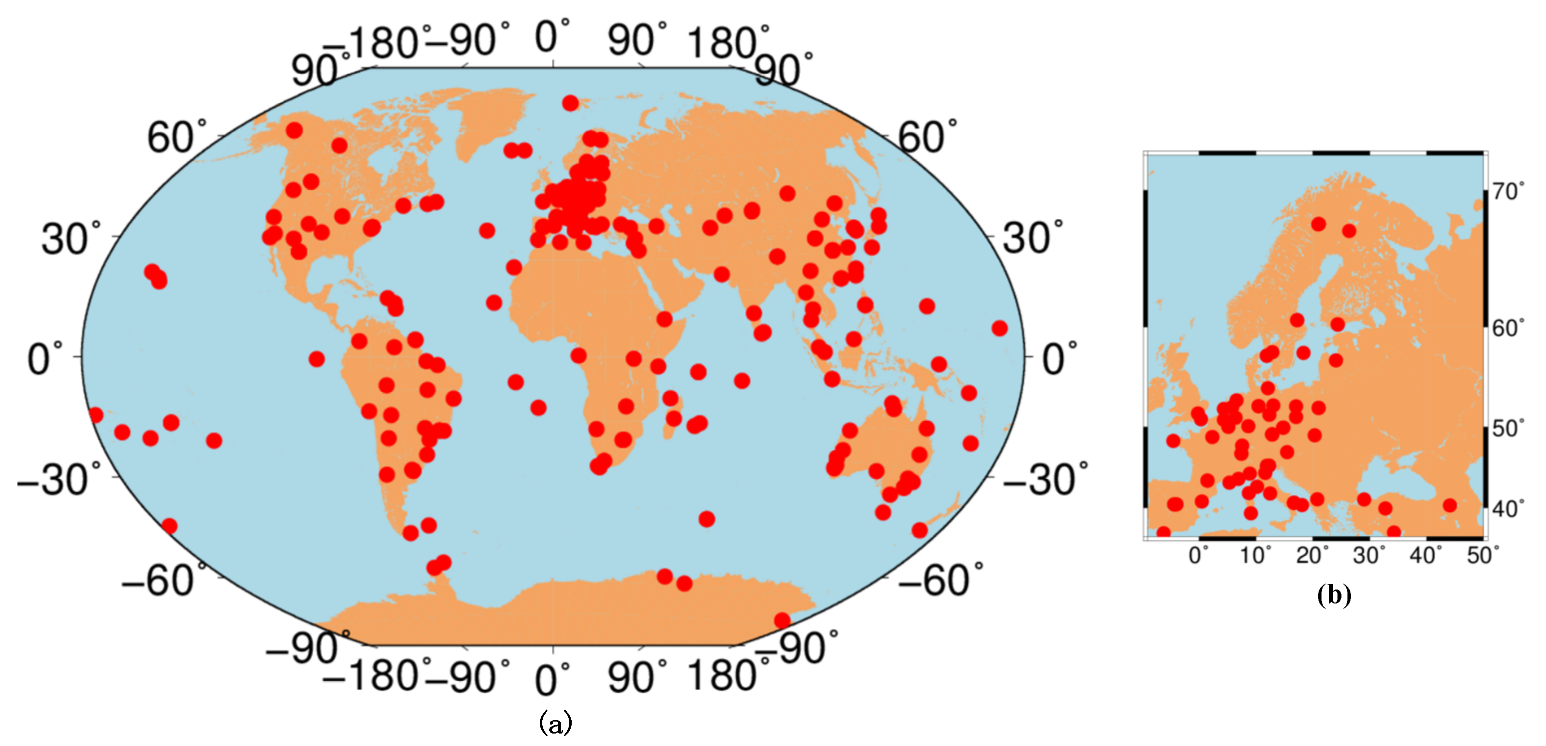
3.1. Experimental Data

As shown in Figure 1, observations from approximately 250 globally distributed stations within the Multi-GNSS Experiment (MGEX) worldwide tracking network were collected to evaluate and analyze the OSBs. The basic information of the processed code observables, including the signal frequencies and observable types, is listed in

Table 1. Observable types and the corresponding frequencies applied for the OSB analyses.

System	Signal	Frequency (MHz)	Observable Types
BDS	B1I	1561.098	C2I
	B1C	1575.42	C1X
	B2a	1176.45	C5X
	B2b	1207.14	C7Z
	B2ab	1191.795	C8X
	B3I	1268.52	C6I
	B2I	1207.14	C7I
GPS	L1	1575.42	C1C, C1W
	L2	1227.60	C2W, C2X, C2S, C2L
	L5	1176.45	C5Q, C5X
Galileo	E1	1575.42	C1C, C1X
	E5a	1176.45	C5Q, C5X
	E5b	1207.14	C7Q, C7X
	E5ab	1191.795	C8Q, C8X
	E6	1278.75	C6C
GLONASS	G1	1602 + k × 9/16, k = −7.... +12	C1C, C1P
	G2	1246 + k × 7/16 k = −7.... +12	C2C, C2P

. A data sampling rate of 30 s was chosen. An elevation cutoff angle of 15° was applied to mitigate the impacts of multipath and mapping function errors at low elevations. Two observation periods were selected to perform our analysis. The first period, covering 1 month from day of year (DOY) 060 to 090 2021, was employed to validate the IONC and DCBC methods. The second period, covering 6 months from DOY 092 to 274 2020, was employed to analyze the characteristics of multi-GNSS satellite and receiver OSBs.

3.2. Validation of the IONC and DCBC Methods for Estimating OSBs

To test the effectiveness of the IONC and DCBC methods presented in Section 2, two performance indicators are employed in this study: (1) the consistency between the OSBs estimated based on the IONC and DCBC method and the external OSB products and (2) the consistency between the DCBs transformed from the estimated OSBs and the corresponding DCBs estimated directly from the raw GNSS observables. Considering the impacts of GNSS networks and receivers on the OSB estimation results [14,24], two experimental schemes are designed to validate the IONC and DCBC methods. The first scheme is designed to validate the DCBC method. In the first scheme, CAS-provided DCBs (CASDCBs) are employed as pseudomeasurements to estimate the OSBs, and the CAS-provided OSBs (CASOSBs) serve as references to evaluate the DCBC-based OSBs (DCBCOSBs). The second scheme is designed to compare the IONC-based OSBs (IONCOSBs) and DCBCOSBs. In the second scheme, the same GNSS observations are used to estimate IONCOSBs and DCBs, which are further employed for DCBC-based OSB estimation.

Since no receiver OSBs are included in the CASOSB products, only the validation of the estimated satellite OSBs is presented in this study. In addition, because the zero-mean condition is imposed on all available satellites to estimate the OSBs, systematic offsets would exist in the daily OSB estimates in the event that the available satellites change. Furthermore, the number of satellites tracked by different sets of stations also varies, and the number of available satellites contributing to the OSB estimation changes if a satellite is newly launched or becomes unavailable. Thus, systematic offsets need to be removed before comparing the OSBs from various sources or different time periods. The realignment procedure reported in the study of Sanz et al. [25] is used to remove the systematic offsets in this study.

3.2.1. Validation of the DCBC Method for Estimating OSBs

Taking the CASDCB products as pseudomeasurements, the OSBs during the period of DOY 060–090 2021 are estimated by the DCBC method. The root mean square (RMS) values of the differences between the CASOSBs and the DCBCOSBs during the test period are depicted in Figure 2. There is no remarkable difference in the RMS values between the CASOSBs and DCBCOSBs. The RMS values of the differences between the two OSB estimates are less than 0.1 ns for GPS and GLONASS and near zero for BDS and Galileo. This comparison demonstrates high consistency between the DCBCOSBs and the CASOSB products.

To verify the consistency between the CASDCBs and the DCB estimates obtained from the OSB estimates, the RMS values of the differences between the DCBs computed based on different OSB estimates and the CASDCBs during the test period are depicted in Figure 3. The RMS values of the differences among the three types of DCB estimates are near 0 for BDS and Galileo, while those of GPS and GLONASS show biases within 0.15 ns and 0.1 ns, respectively. The agreement achieved between the CASDCBs and the DCB estimates obtained from the two types of OSB estimates demonstrates the effectiveness of the DCBC OSB estimation method.

3.2.2. Validation of the IONC Method for Estimating OSBs

To validate the effectiveness of the IONC method, OSBs are estimated by the IONC method based on observations collected from the selected stations shown in Figure 1. The DCBs estimated based on the same sets of observations (GIMDCB) are employed as pseudomeasurements to obtain the DCBCOSBs. Figure 4 shows the RMS values of the differences between the IONCOSBs and DCBCOSBs. The maximum differences between the two OSB estimates for GLONASS are larger than those of the other satellite systems. For GPS, the C1W and C1C signals achieve the smallest difference and largest difference, respectively, between the IONCOSB and DCBCOSB. For BDS and Galileo, the OSB differences between the IONC method and DCBC method for signals at the first frequency are smaller than those for signals at other frequencies. For Galileo, the differences between the two types of OSB estimates for the pilot signals are less than those for the combined signals. In addition, the RMS values of the difference between the IONCOSB and DSBOSB for the four satellite systems are less than 0.15 ns, demonstrating encouraging consistency between the IONC method and DCBC method.

To further confirm the consistency between the DCBs directly estimated by correcting the ionospheric delay using the IGS-combined GIM products and those obtained from different OSB estimates, the RMS values of the differences among the three different DCB estimates are depicted in Figure 5. The types of BDS DCBs shown in this figure are formed with respect to the B1I signal, different from the CAS-provided BDS DCB products. Although the DCBs generated based on the DCBCOSB exhibit better consistency with the GIM-based DCB estimates, the maximum difference between the GIM-based DCB estimates and the DCBs generated based on the IONC OSBs is less than 0.15 ns, showing the effectiveness of the IONC OSB estimation method.

3.3. Characteristics of the Multi-GNSS Satellite OSBs

The consistency among the IONCOSB and DCBCOSB and the CASOSBs is validated in Section 3.2. To understand the characteristics of the multi-GNSS satellite OSBs, Figure 6, Figure 7, Figure 8 and Figure 9 depict the mean values of the DCBCOSBs for all operational satellites during the second test period. These satellites are aligned across a period of 6 months, and individual satellites are labeled by their space vehicle number (SVN) for unambiguous identification and are sorted by block types on the horizontal axis.

The mean OSB estimates for the GPS satellites shown in Figure 6 reveal that the GPS OSB estimates are confined to a range of −19.61 to 21.51 ns. Consistent with the findings of [11,14], the GPS OSB estimates appear to depend on the block type. The OSB estimates from Block IIF satellites are significantly larger than those from the other block types, while the ranges of the OSBs within Blocks II-A and IIR-M are similar, and the satellite OSB estimates at the same frequency show agreement with each other. In addition, the signals supported by satellites are also related to the block type. For example, all Block IIR-A satellites and Block IIR-B satellites, except SVN G060, are unable to support the C2S, C2X and C2L signals, whereas the third L5 civil signals, i.e., C5Q and C5X, are transmitted by the Block IIF, IIA and IIIA and SVN G060 satellites.

The OSB estimates for the GLONASS satellites presented in Figure 7 reveal that the OSBs for all GLONASS satellites are confined to the range of −10.87 to 20.64 ns. Unlike GPS, however, there is no remarkable dependence on the satellite type within the GLONASS OSB estimates. The OSBs of the signals at the same frequency exhibit agreement for the individual GLONASS satellites.

As shown in Figure 8, the OSB estimates for the BDS satellites are divided into geostationary Earth orbit (GEO) satellites (BDS-2G), medium Earth orbit (MEO) satellites (BDS-2M and BDS-3M) and inclined geosynchronous orbit (IGSO) satellites (BDS-2I and BDS-3I). The OSBs for the BDS-3M satellites exhibit a larger range than those of the other satellites, and the BDS OSB estimates for the B1I and B1C signals show similar bias patterns. The satellite OSBs for the B2a, B2b and B2ab signals also achieve similar estimates. Other than the C214 satellite, which exhibits large OSB estimates, the OSB estimates for most satellites are smaller than 37 ns.

The OSB estimates shown in Figure 9 reveal that the Galileo satellite OSB estimates, except for those from the SVN E205 satellite, are confined to the range of −29.15 to 6.96 ns. In addition, the OSB estimates for the pilot and combined signals at the same frequencies exhibit similar bias patterns.

To understand the stability of the satellite OSB estimates, the GPS C1W, GLONASS C1P, BDS C2I and Galileo C1X signals are selected as examples. The time series of the OSB estimates for satellites whose OSBs exhibit abnormal variations during the test period, are depicted in Figure 10. Several gaps due to discontinuous data are detected. Abnormal variations or significant discontinuities can be detected for the following satellites: G060 on DOY 161, C204 on DOY 135, R731 on DOY 160, R735 on DOY 100 and E205 on DOY 272. Similar discontinuities have also been observed in DCB and OSB time series by previous studies [11,26], which attributed this phenomenon to flex power or the occurrence of satellite maneuvers or onboard equipment maintenance in the constellation. Thus, although the OSBs of most satellites can remain stable over long time periods, it is better not to directly use the OSBs estimated on previous days, since significant jumps may occur in the OSB values between two consecutive days.

To further study the stability of the OSBs for different signals, the mean standard deviations (STDs) of the satellite OSB estimates during the second test period are shown in Figure 11, Figure 12, Figure 13 and Figure 14. The satellite OSBs for BDS and GLONASS show inferior stability to those for GPS and Galileo. For GPS, the OSB estimates for Block IIF satellites present inferior stability to those of the other block types. Furthermore, the GPS OSBs for signals at the first frequency show superior stability to those for signals at other frequencies, and the mean STDs of the satellite OSBs for the new L2 civil signals and L5 signals are on the same level.

As shown in Figure 12, the OSB estimates for the IGSO satellites in the BDS2 and BDS3 constellations show better stability than those for the GEO and MEO satellites. The stability of the OSBs for different satellites is in accordance with the results for the DCBs reported in Li et al. [6]; this phenomenon can be attributed to the notion that IGSO satellites have longer observation arcs and wider geographic coverage than other satellites. For BDS2, the OSB estimates for GEO satellites have the largest STDs. Moreover, the OSB estimates for the B1I and B1C signals show better stability than those for the other signals.

For GLONASS, the stability of the OSB estimates for the signals in the G1 frequency band outperforms those of the signals in the G2 frequency band. The GLONASS OSB estimates show larger STDs than those of GPS signals, which is consistent with the findings of Wang et al. [14] and Villiger et al. [11].

As shown in Figure 14, the STDs of the OSB estimates of the signals at the E1 frequencies are less than 0.15 ns, representing better stability than those of the signals at other frequencies. Additionally, compared to the STDs of the GPS, BDS and GLONASS OSBs, the STDs of the Galileo OSBs among different satellites show smaller variations.

Considering that the accuracy of the GIM products varies with the solar activity level, the accuracy of the OSB estimates tends to be different at various solar activity levels. To understand the precision variation of OSB estimates during different solar cycle periods, the mean STDs of the OSB estimates for the period of DOY 092 to 274 2020 (lower solar activity) and DOY 092 to 274 2015 (higher solar activity) are summarized in

Table 2. Mean STDs of the satellite OSB estimates for the period of DOY 092 to 274 2020 (unit: ns).

GPS	C1C	C1W	C2W	C2X	C2S	C2L	C5Q	C5X
	0.14	0.12	0.19	0.2	0.21	0.21	0.21	0.21
GLONASS	C1C	C1P	C2C	C2P
	0.19	0.18	0.29	0.29
BDS	C2I	C6I	C7I	C1X	C5X	C7Z	C8X
	0.23	0.34	0.34	0.23	0.3	0.27	0.28
Galileo	C1C	C1X	C5Q	C5X	C6C	C7Q	C7X	C8Q	C8X
	0.1	0.11	0.19	0.2	0.16	0.17	0.18	0.18	0.2

and

Table 3. Mean STDs of the satellite OSB estimates for the period of DOY 092 to 274 2015 (unit: ns).

GPS	C1C	C1W	C2W	C2X	C2S	C2L	C5Q	C5X
	0.15	0.15	0.26	0.27	0.26	0.32	0.28	0.27
GLONASS	C1C	C1P	C2C	C2P
	0.28	0.26	0.54	0.44
BDS	C2I	C6I	C7I
	0.45	0.63	0.53
Galileo	C1C	C1X	C5Q	C5X	C7Q	C7X	C8Q	C8X
	0.22	0.26	0.41	0.30	0.39	0.31	0.38	0.29

, respectively. Since BDS3 signals and the Galileo C6C signal have no observables in 2015, their information is not shown in Table 3. A comparison of Table 2 and Table 3 shows a significant increase in STD values in response to the increase in the solar activity level. The inferior stability of OSBs in 2015 is related to the larger bias in the GIM-derived ionosphere delay and fewer available observations due to the smaller number of contributed stations during higher solar activity than during lower solar activity.

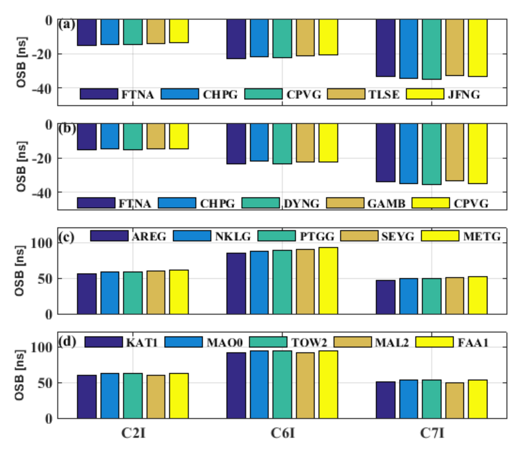
3.4. Characteristics of the Multi-GNSS Receiver OSBs

To understand the characteristics of the multi-GNSS receiver OSBs, the mean values and STDs of the DCBCOSBs are calculated during the second test period. Previous studies have shown that receiver DCBs are related to the receiver type, firmware version and antenna type [3,6]. To analyze the impacts of the hardware on the magnitudes of receiver OSB estimates, the BDS C2I, C7I and C6I signals are taken as examples. Figure 15 shows histograms of the average receiver OSB estimates for the selected stations in four groups equipped with the same types of receivers and antennas and the same firmware version.

Table 4. STDs and mean values of the receiver DCB estimates with the same receiver type, firmware version and receiver antenna type (unit: ns).

Group	Receiver Type	Firmware Version	Antenna Type	C2I		C6I		C7I
				Mean	STD	Mean	STD	Mean	STD
a	TRIMBLE NETR9	5.43	TRM59800.00	−14.29	0.55	−21.63	0.82	−33.61	0.91
b	TRIMBLE NETR9	5.45	TRM59800.00	−14.88	0.41	−22.48	0.62	−34.41	0.96
c	SEPT POLARX5	5.3.2	TRM59800.00	58.7	1.98	88.94	3.01	49.63	2.23
d	SEPT POLARX5	5.3.2	LEIAR25.R4	61.55	1.17	93.25	1.77	52.33	1.83

shows the receiver information of the four groups of stations and the corresponding statistical results. Note that since the firmware versions for stations FTNA and CHPG both changed on DOY 145 in 2021, the two stations both appear in subfigures (a,b) of Figure 15. The significant differences between different groups were calculated using a T-test, and the threshold for statistical significance was set to p < 0.05. There are significant differences in the OSB estimates between receivers from different manufacturers, and no significant difference was observed between group (a) and group (b). In contrast, the OSB estimates for receivers with the same types of receivers and antennas and the same firmware version are determined to have similar values.

To further analyze the effects of equipment from different manufacturers, including different types of receivers and antennas and firmware versions, on receiver OSB estimates, the OSBs at stations METG, SPT0 and AGGO and KIT3 are selected as examples. Figure 16, Figure 17, Figure 18 and Figure 19 show the relevant time series of receiver OSB estimates.

Table 5. Information on the receiver and antenna types and receiver firmware versions used for stations METG, SPT0, AGGO and KIT3.

Station	Periods	Receiver Type	Antenna Type	Firmware Version
METG	DOY 092–147	TRIMBLE NETR9	TRM59800.00	5.43
	DOY 148–218	TRIMBLE NETR9	TRM59800.00	5.45
	DOY 219–244	SEPT POLARX5	TRM59800.00	5.3.2
AGGO	DOY 092–130	SEPT POLARX4TR	LEIAR25.R4	2.9.6
	DOY 131–171	LEICA GRX1200+GNSS	LEIAR25.R4	8.71
	DOY 172–274	LEICA GRX1200+GNSS	LEIAR25.R4	9.20
KIT3	DOY 092–241	JAVAD TRE_G3TH DELTA	JAV_RINGANT_G3T	3.7.9
	DOY 242–268	SEPT ASTERX4	SEPCHOKE_B3E6	4.7.1
	DOY 269–274	SEPT ASTERX4	SEPCHOKE_B3E6	4.8.0
SPT0	DOY 093–226	SEPT POLARX5TR	JNSCR_C146-22-1	5.3.0
	DOY 227–244	SEPT POLARX5TR	TRM59800.00	5.3.0

lists the corresponding configuration information before and after changing the devices for these stations. The results show that the receiver OSB estimates are relatively stable, except for the jumps caused by changes in the receiver hardware device.

Consistent with the changes in the receiver types at stations METG, AGGO and KIT3, significant variations in the receiver OSB estimates for different GNSS constellations are detected among the three stations. For stations METG and AGGO, the antenna types remain unchanged when the receiver type changes; thus, the variations in the receiver OSBs are driven by a change in receiver type instead of a change in antenna type. For station AGGO, the Galileo receiver OSB estimates between signals at different frequency bands show different variation trends. For station KIT3, when the receiver type changes from JAVAD TRE_G3TH to SEPT ASTERX4, the tracked signals shift from C1X and C5X to C1C, C5Q, C6C, C7Q and C8Q. Likewise, changes in the signal types tracked before and after a change in the receiver type can also be found at station METG.

Consistent with the changes in the antenna type at station SPT0, the receiver OSB estimates for both the BDS and the GLONASS systems exhibit significant variations. When the firmware version at station AGGO changes, the receiver OSB estimates for all GPS signals and the Galileo C1C and C5Q signals remain unchanged, whereas the Galileo receiver OSB estimates for the C7Q and C8Q signals show abnormal variations. For stations METG and KIT3, the receiver OSB estimates for all signals remain unchanged when the firmware version changes.

Based on the analysis for the four selected stations, it can be concluded that changes in the types of receivers and antennas can cause variations in the receiver OSB estimates. In addition, the impacts of changes in the firmware version on the receiver OSB estimates vary for signals at different frequency bands and different GNSS constellations.

Next, to investigate the stability of the receiver OSB estimates for signals in different frequency bands, Figure 20 depicts the mean STDs of the receiver OSB estimates for the second test period, during which there is no change in the receiver hardware device. The mean STDs of the OSB estimates for the four GNSS constellations range from 0.43 to 0.86 ns, showing inferior stability to those of the satellite OSBs. Moreover, the STDs of the receiver OSBs in the first frequency band show better stability than those at the other frequencies.

3.5. Comparison of the Satellite OSBs Estimated Based on the CAS- and DLR-Provided DCB Products

As demonstrated in Section 2.2, the DCBC method can be employed to estimate satellite and receiver OSBs directly based on external DCBs. Multi-GNSS DCB products have been provided by CAS and DLR since 2014, meaning that long-term OSBs can be estimated and further analyzed based on CAS- and DLR-provided DCB products. However, since both the estimation method and GNSS tracking networks employed for the estimation of the CAS- and DLR-provided DCB products diverge, the accuracies of the DCB products and the derived OSB estimates tend to differ.

To compare the differences in the DCBCOSBs caused by different DCB products, the mean RMS values of the satellite OSB differences estimated based on the CAS- and DLR-provided DCB products during the second test period are plotted in Figure 21. The RMS values of the differences between the two OSB estimates for the GPS C1W, BDS C2I, Galileo C1X and GLONASS C1P signals exhibit superior consistency to the other signals within each constellation. Furthermore, the OSB estimates between the two DCB products for GPS and Galileo exhibit better consistency than those between the products for BDS and GLONASS. The RMS differences in the OSBs estimated based on the CAS- and DLR-provided DCB products are 0.32 ns for GPS, 0.45 ns for BDS, 0.39 ns for GLONASS and 0.22 ns for Galileo.

To evaluate the stability of the two types of OSBs, Figure 22 displays the STDs for the two satellite OSB estimates during the second test period. The mean STDs of the GPS OSBs estimated based on the CAS- and DLR-provided DCBs are at the same level of 0.18 ns. For the OSBs estimated based on the CASDCBs, the mean STDs of the OSB estimates for GLONASS, BDS and Galileo are 0.18, 0.31 and 0.2 ns, respectively; likewise, for the OSBs estimated based on the DLR-provided DCBs, the mean STDs of the OSB estimates for GLONASS, BDS and Galileo are 0.29, 0.22 and 0.22 ns, respectively. Overall, there is no remarkable difference in the stability of the OSB estimates from the CAS- and DLR-provided DCB solutions.

4. Discussion and Conclusions

This article applies two computationally efficient methods for the generation of multi-GNSS satellite and receiver OSBs. In the IONC method, satellite and receiver OSBs are estimated simultaneously based on GNSS data obtained from the MGEX network by correcting the ionospheric delay using external GIM products. In the DCBC method, satellite and receiver OSBs are directly converted from external DCB products, which makes it possible to investigate the characteristics of long-term satellite and receiver OSBs based on existing DCB products. The consistency of the IONC and DCBC methods with the traditional method is confirmed, and the characteristics of the estimated OSBs are discussed. The conclusions are summarized as follows:

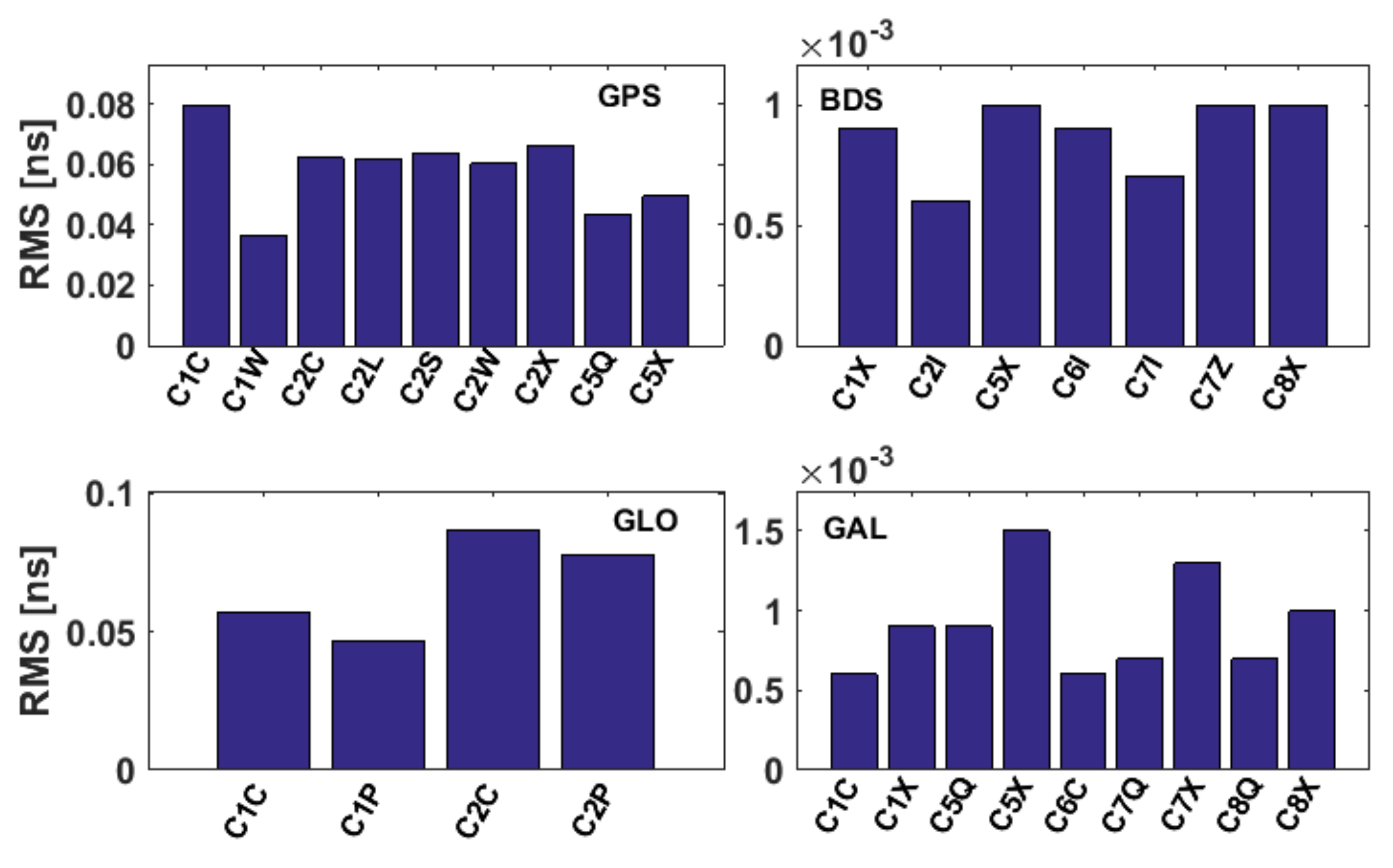
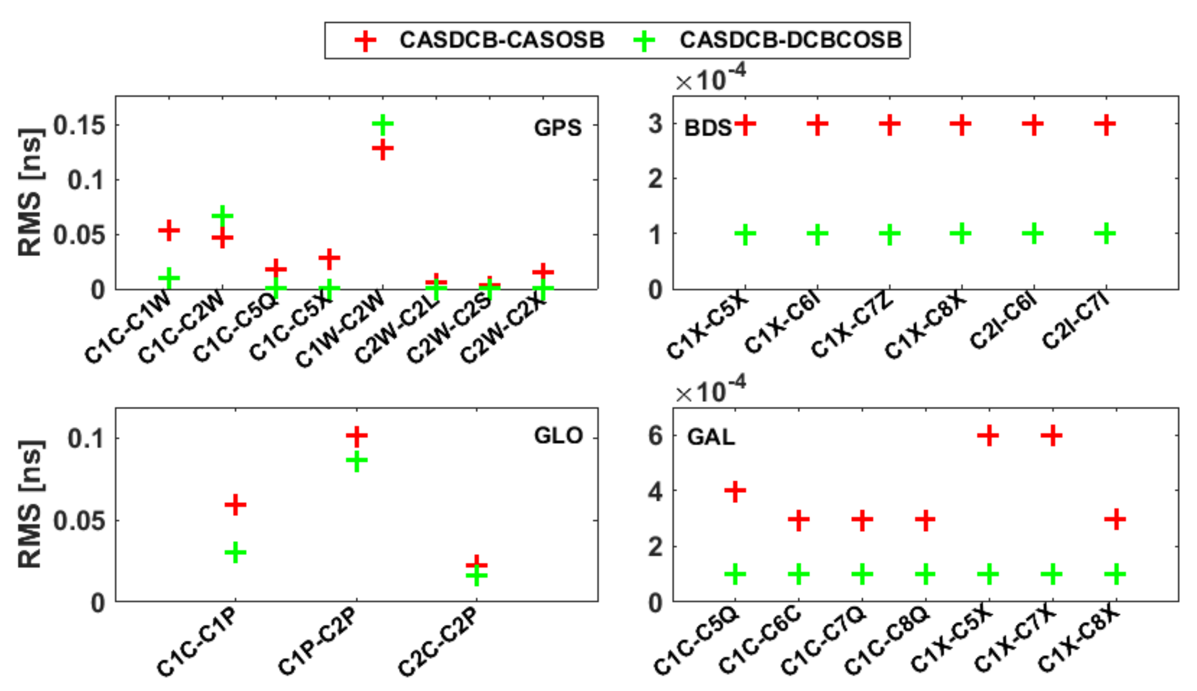
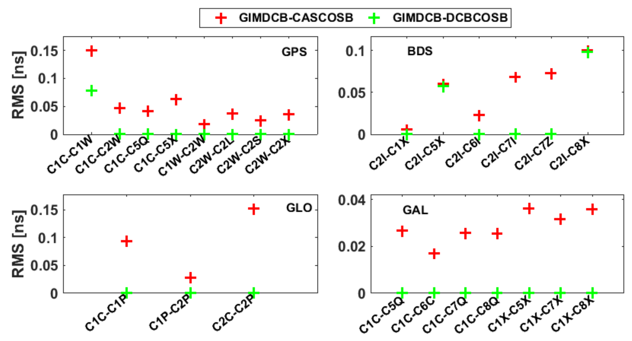
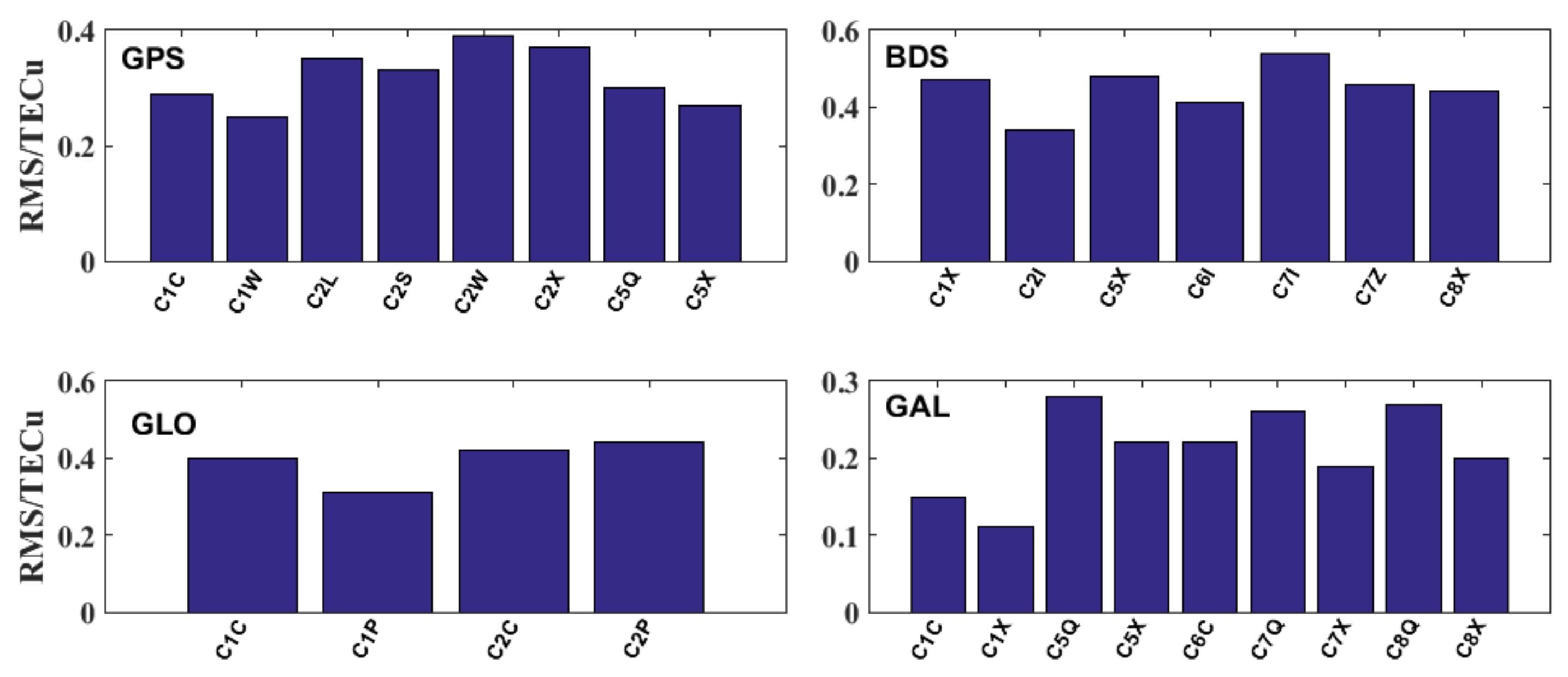
• The RMS values of the differences between the DCBC-based satellite multi-GNSS OSB estimates and those in the CAS-provided product for the four constellations are less than 0.1 ns. Furthermore, consistency between the IONCOSBs and DCBCOSBs is achieved, with RMS values of less than 0.15 ns.
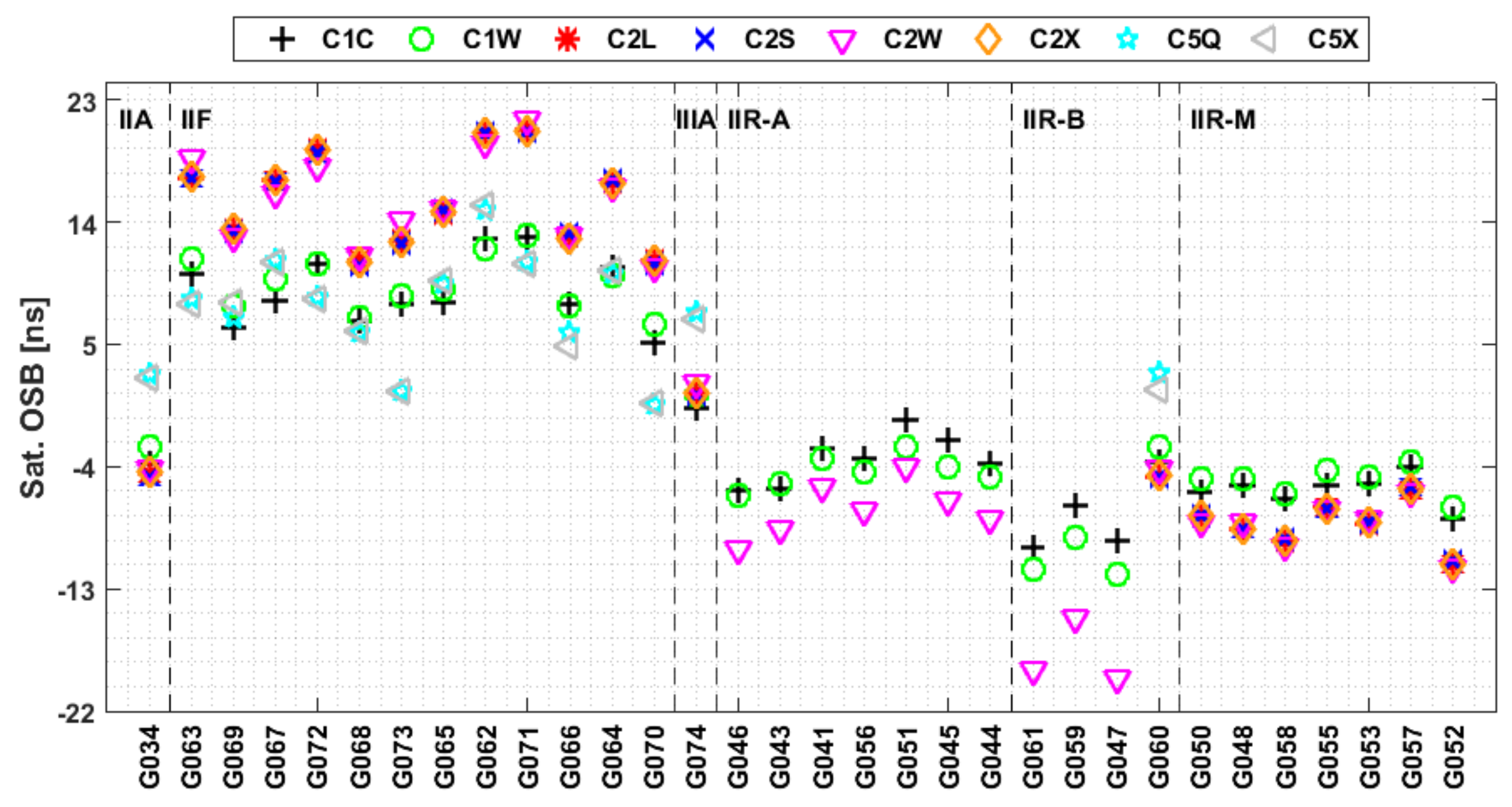
• Consistent with previous studies, the GPS satellite OSB estimates are related to the block type, and GNSS signals at the same frequency exhibit very similar OSB estimates. The stability of OSB estimates is determined to be worse under high compared to low solar conditions.
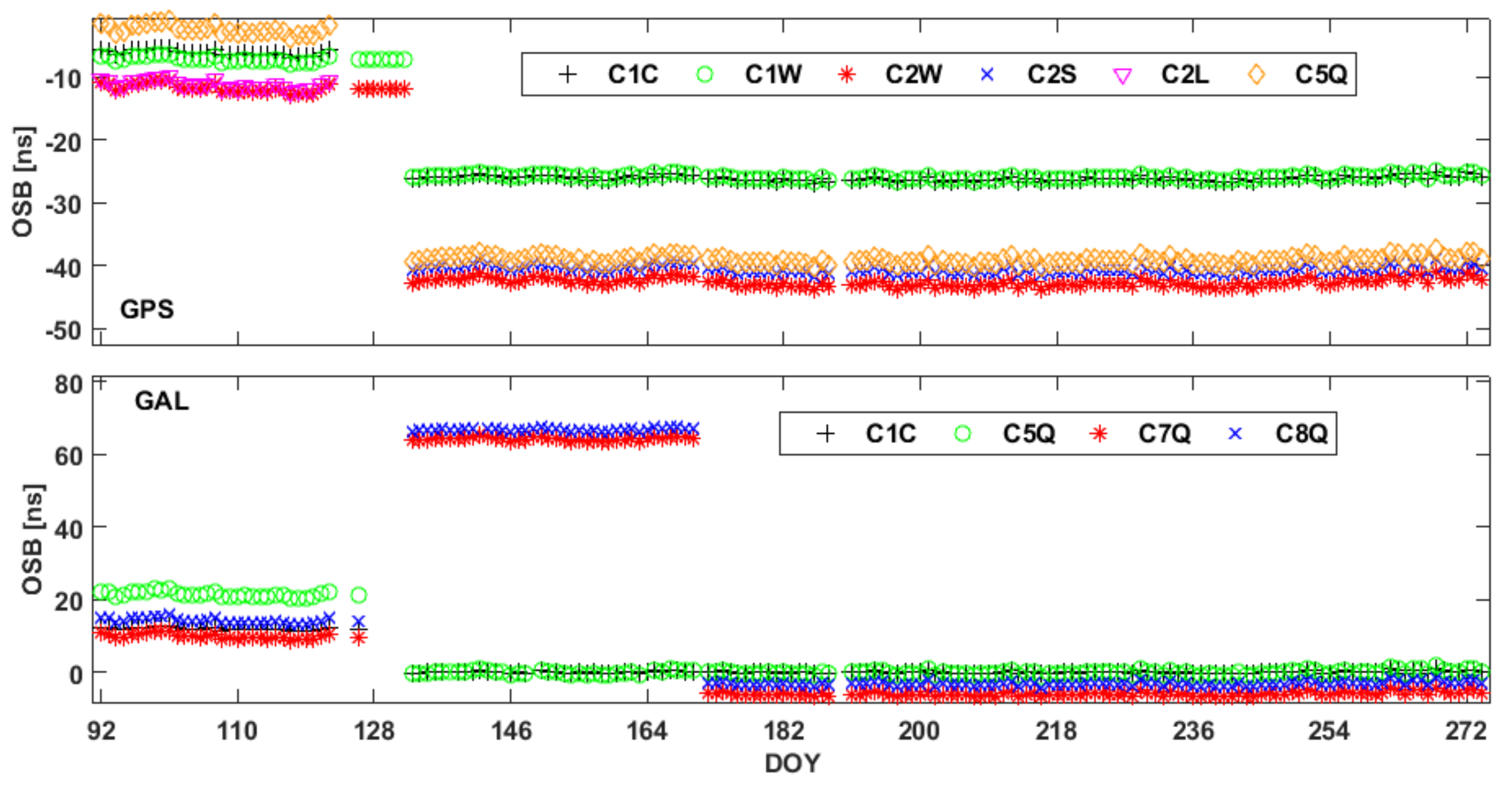
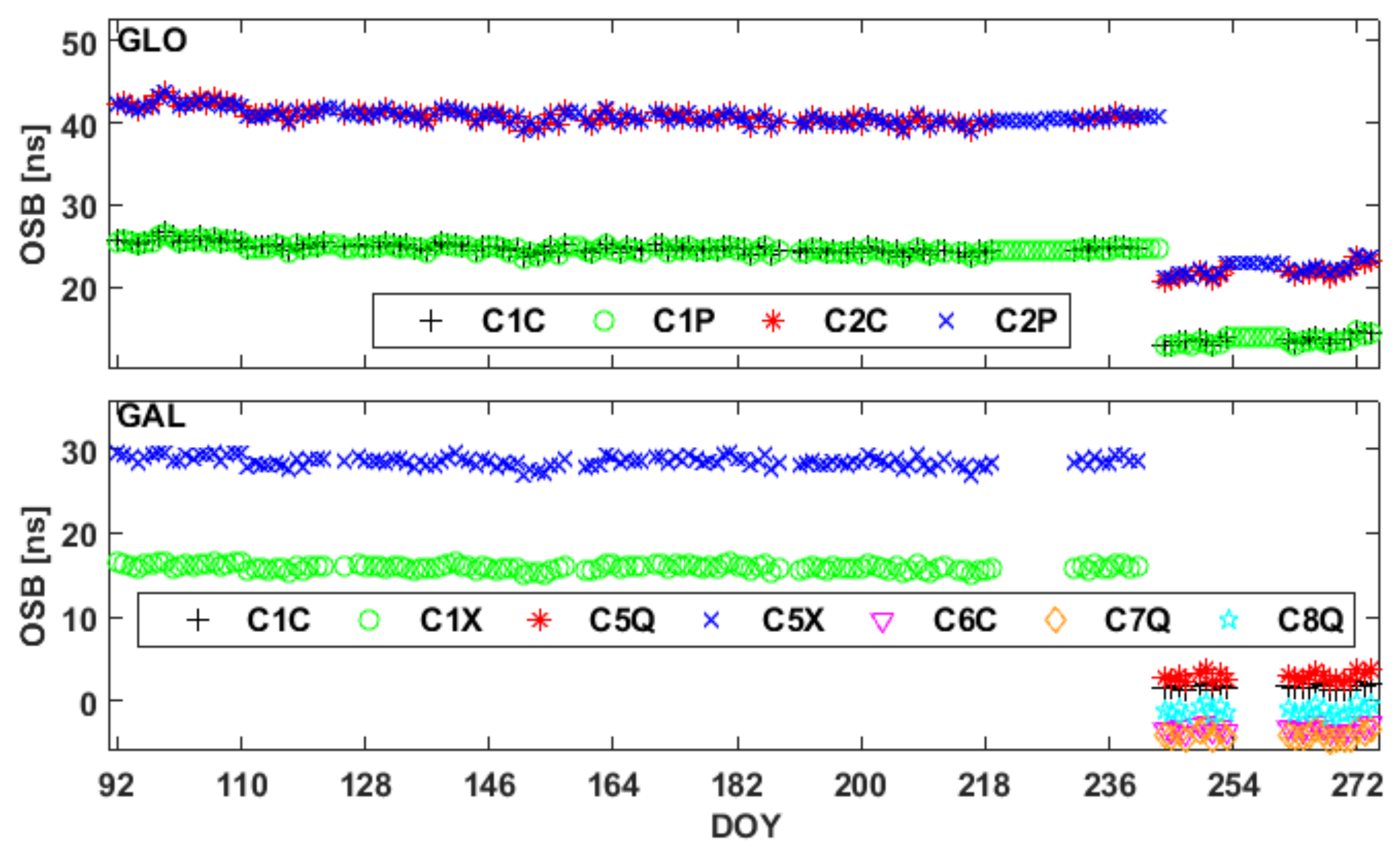
• Although most of the satellite OSB estimates remain stable over long time periods, significant jumps may occur in satellite OSB estimates between two consecutive days.
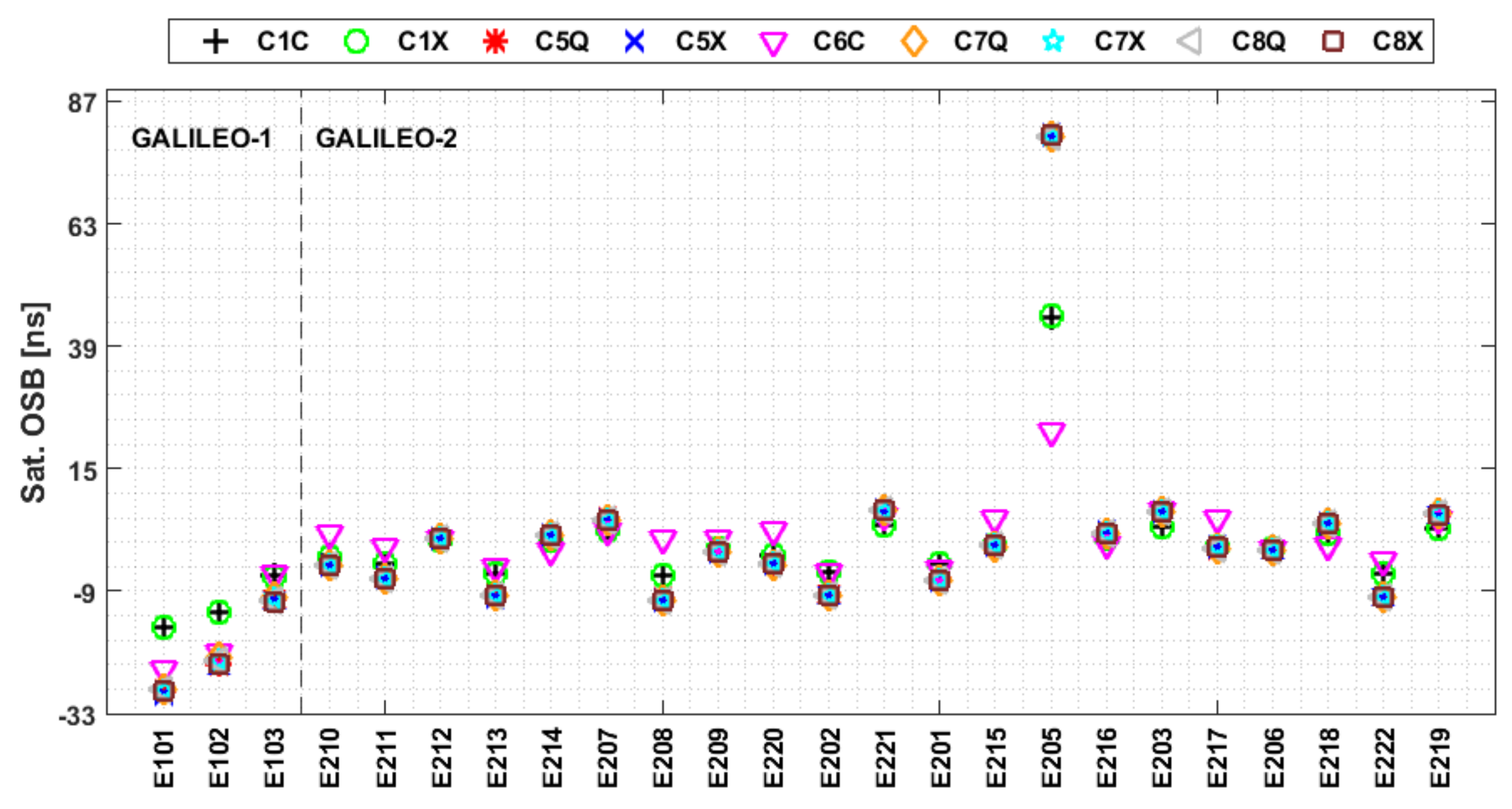
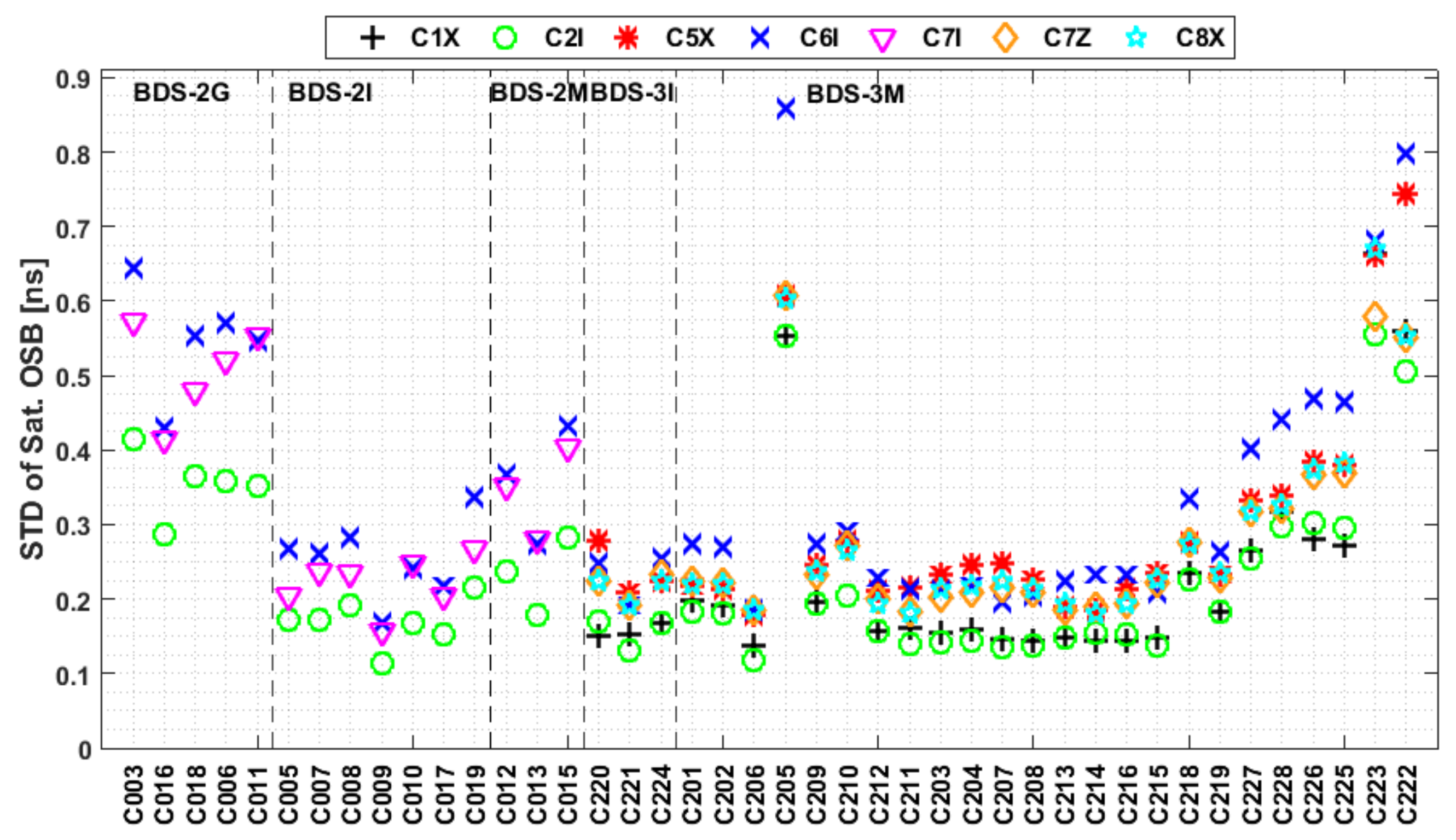
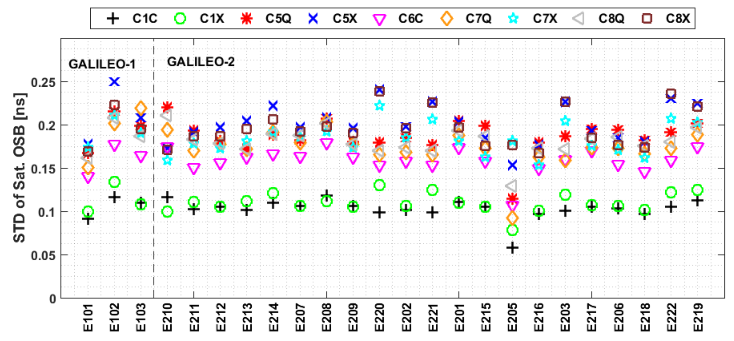
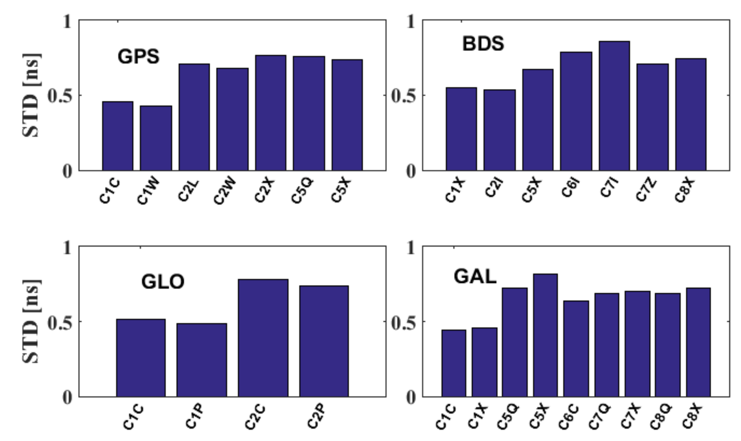
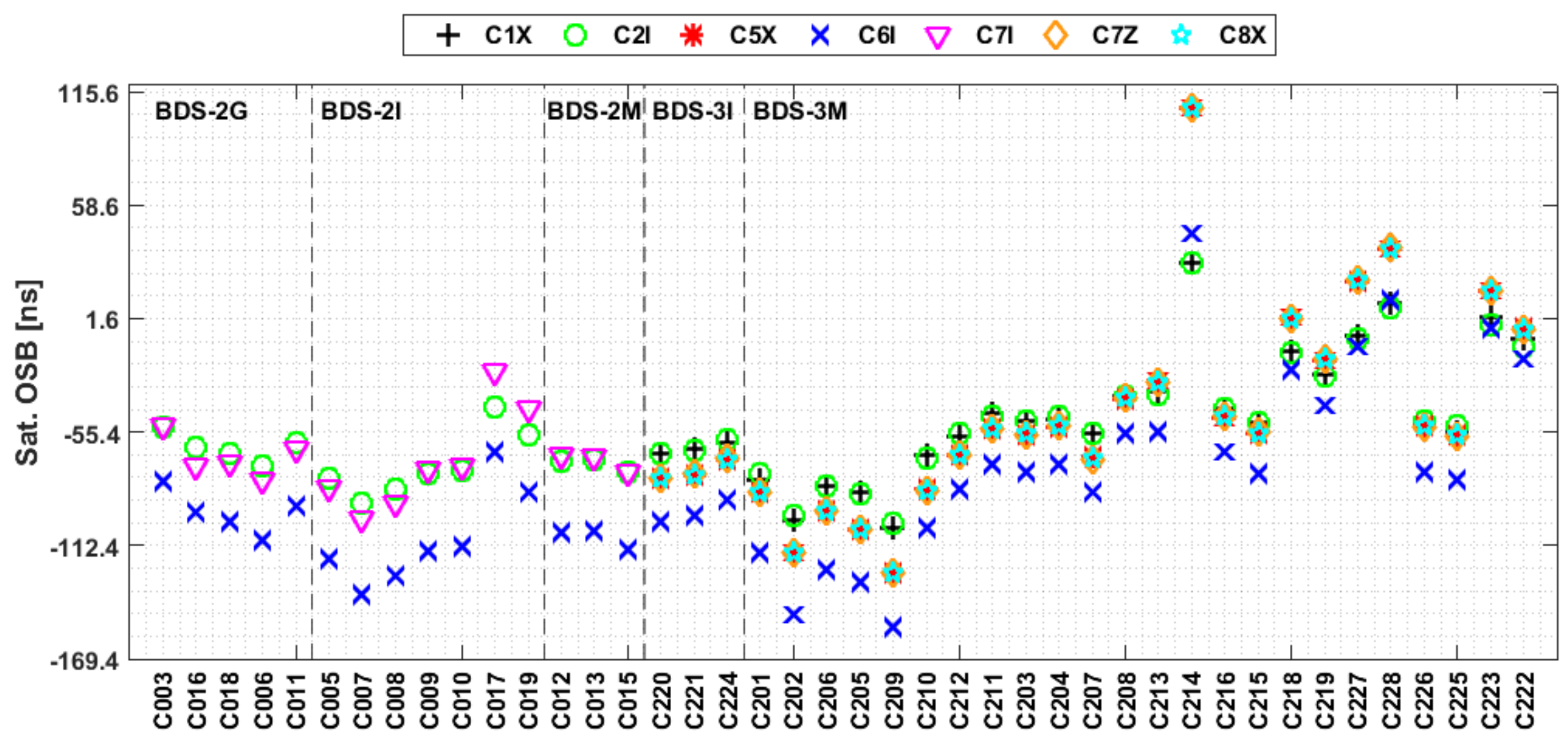
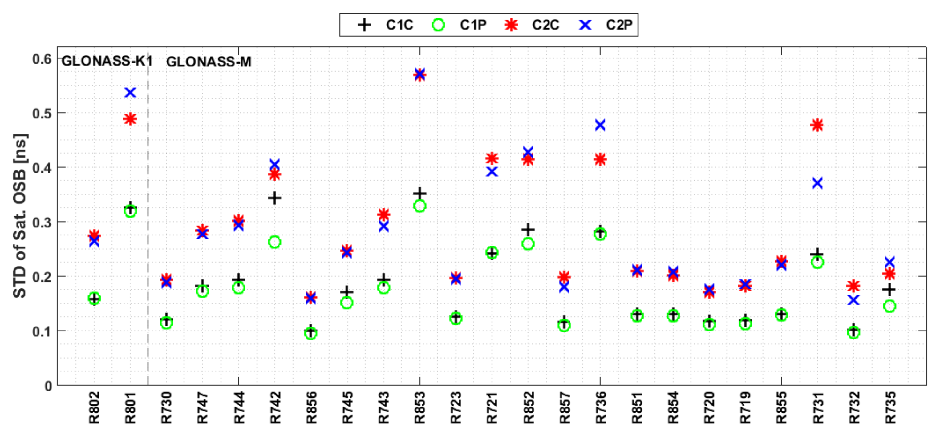
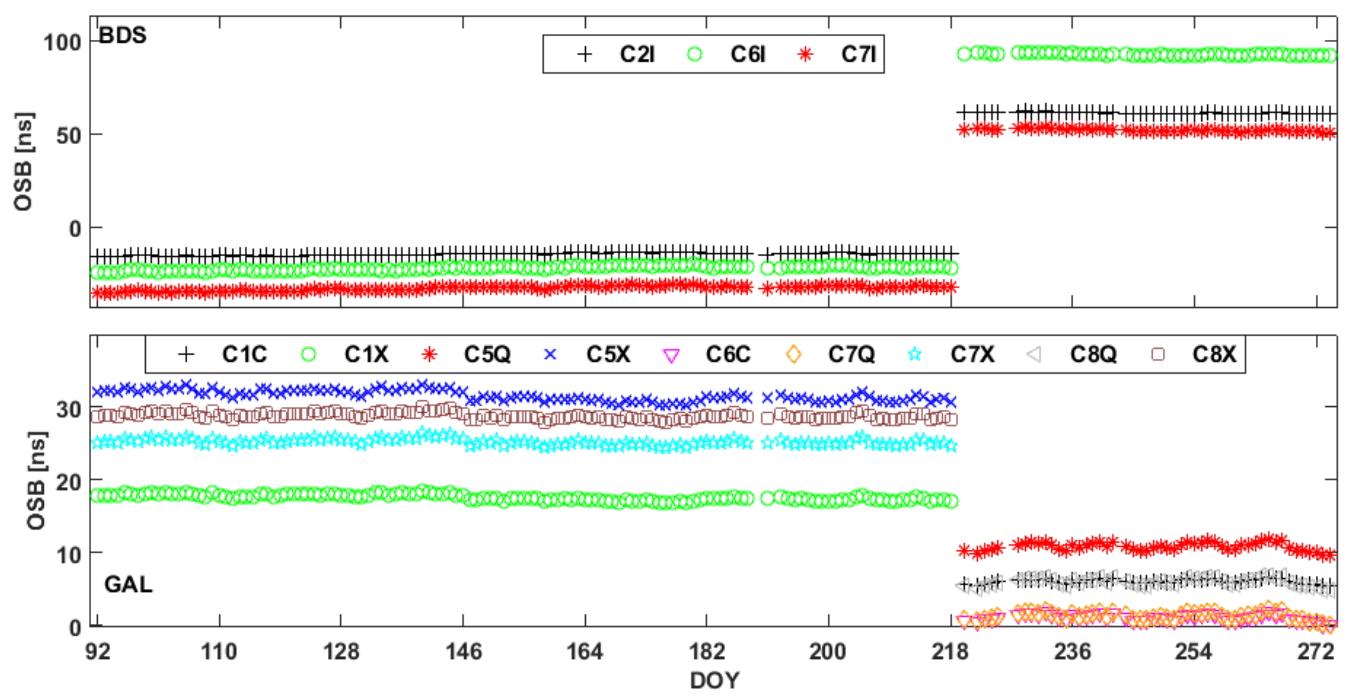
• The satellite and receiver OSB estimates for signals in the first frequency band show superior stability to those at other frequencies. Additionally, the OSB estimates for GPS and Galileo show better stability than those of BDS and GLONASS, and the BDS satellite OSB estimates for IGSO satellites show better stability than those for MEO and GEO satellites for both BDS2 and BDS3.
• Variations in the types of receivers and antennas impact the receiver OSB estimates. Moreover, the influence of the firmware version on the OSB estimates for signals at different frequency bands may differ.
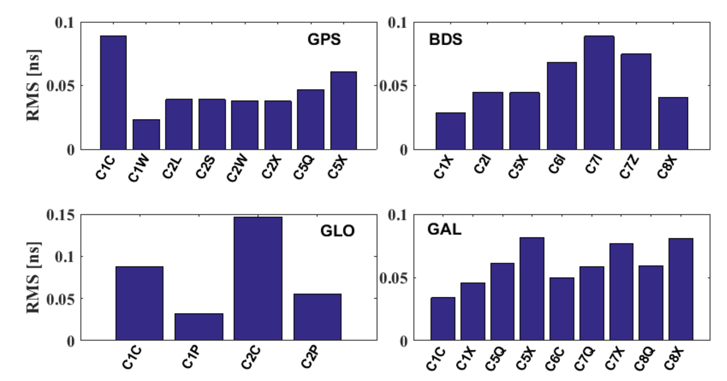
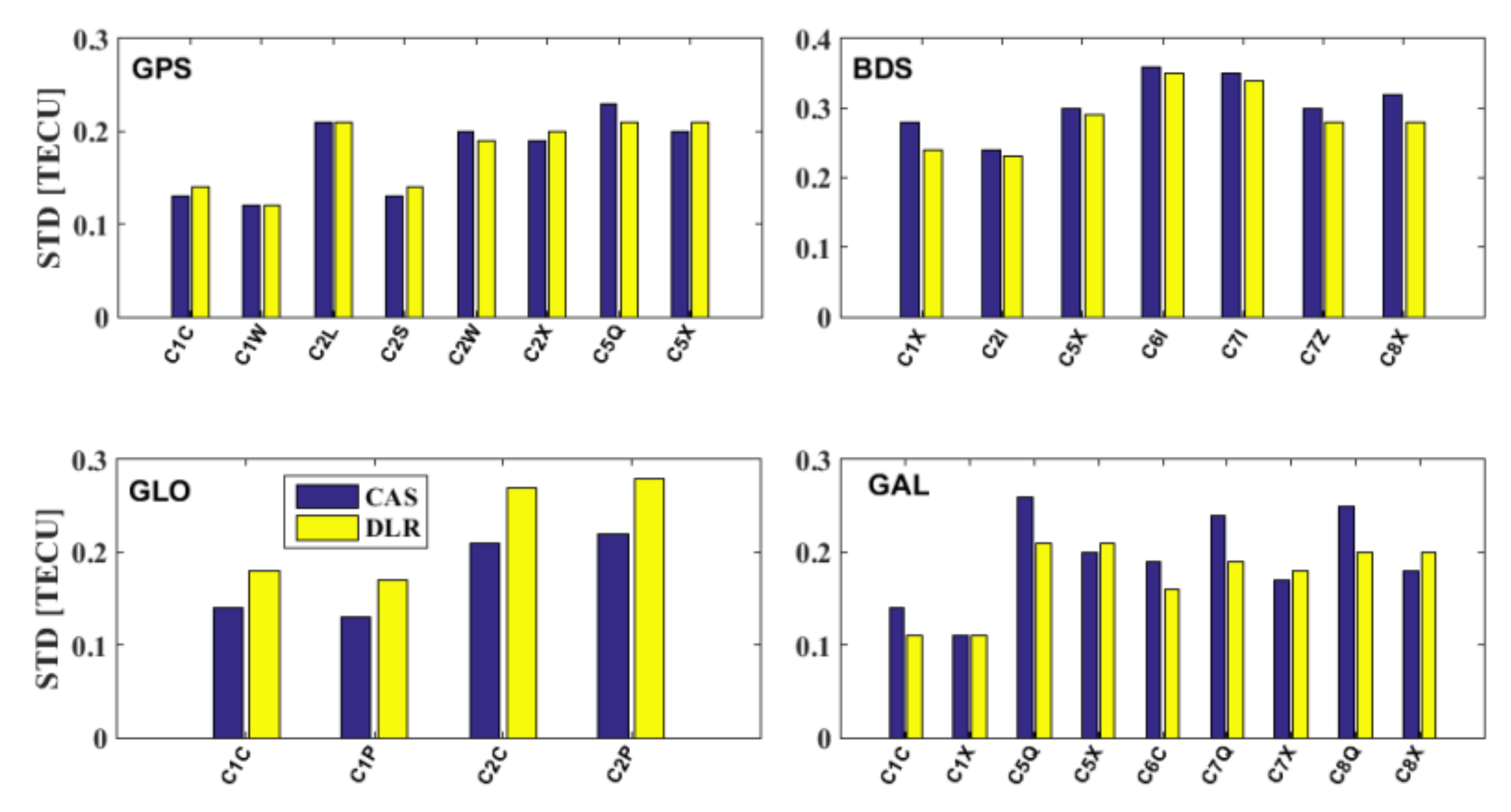
• The RMS values of the differences in the DCBCOSBs estimated based on the CAS- and DLR-provided DCBs are less than 0.45 ns.

For the sake of convenience, both satellite and receiver OSBs are assumed to be constant over a period of 24 h in this study, implying that the estimated OSBs are the mean values of the daily OSBs. However, previous studies have demonstrated that the variability of receiver code bias is closely associated with temperature variations and hardware updates [27,28]. The intraday variations in receiver OSBs may be diminished by averaging the receiver OSBs on a daily basis. Hence, further investigation is required to understand the intraday variations in OSBs. In addition, conclusions regarding the characteristics of multi-GNSS satellite and receiver OSBs are drawn from an analysis based on data spanning only 6 months in 2020. With the increasing diffusion of low-cost differential receivers [29,30,31], future research should be performed with a longer observation period and more types of signals.

References

1. Zhang, Z.; Lou, Y.; Zheng, F.; Gu, S. ON GLONASS pseudo-range inter-frequency bias solution with ionospheric delay modeling and the undifferenced uncombined PPP. J. Geod. 2021, 95, 32. [Google Scholar] [CrossRef]
2. Håkansson, M.; Jensen, A.B.O.; Horemuz, M.; Hedling, G. Review of code and phase biases in multi-GNSS positioning. GPS Solut. 2016, 21, 849–860. [Google Scholar] [CrossRef] [Green Version]
3. Li, M.; Yuan, Y.B.; Wang, N.B.; Li, Z.S.; Li, Y.; Huo, X.L. Estimation and analysis of Galileo differential code biases. J. Geod. 2017, 91, 279–293. [Google Scholar] [CrossRef]
4. Li, W.; Wang, G.; Mi, J.; Zhang, S. Calibration errors in determining slant Total Electron Content (TEC) from multi-GNSS data. Adv. Space Res. 2019, 63, 1670–1680. [Google Scholar] [CrossRef]
5. Banville, S.; Geng, J.; Loyer, S.; Schaer, S.; Springer, T.; Strasser, S. On the interoperability of IGS products for precise point positioning with ambiguity resolution. J. Geod. 2020, 94, 10. [Google Scholar] [CrossRef]
6. Li, M.; Yuan, Y. Estimation and Analysis of BDS2 and BDS3 Differential Code Biases and Global Ionospheric Maps Using BDS Observations. Remote Sens. 2021, 13, 370. [Google Scholar] [CrossRef]
7. Roma-Dollase, D.; Hernández-Pajares, M.; Krankowski, A.; Kotulak, K.; Ghoddousi-Fard, R.; Yuan, Y.; Li, Z.; Zhang, H.; Shi, C.; Wang, J.; et al. Consistency of seven different GNSS global ionospheric mapping techniques during one solar cycle. J. Geod. 2017, 92, 691–706. [Google Scholar] [CrossRef] [Green Version]
8. Wang, N.B.; Yuan, Y.B.; Li, Z.S.; Montenbruck, O.; Tan, B.F. Determination of differential code biases with multi-GNSS observations. J. Geod. 2016, 90, 209–228. [Google Scholar] [CrossRef]
9. Montenbruck, O.; Hauschild, A.; Steigenberger, P. Differential Code Bias Estimation using Multi-GNSS Observations and Global Ionosphere Maps. Navigation 2014, 61, 191–201. [Google Scholar] [CrossRef]
10. Sleewagen, J.; Clemente, F. Quantifying the pilot-data bias on all current GNSS signals and satellites. In Proceedings of the IGS Workshop, Wuhan, China, 29 October–2 November 2018. [Google Scholar]
11. Villiger, A.; Schaer, S.; Dach, R.; Prange, L.; Sušnik, A.; Jäggi, A. Determination of GNSS pseudo-absolute code biases and their long-term combination. J. Geod. 2019, 93, 1487–1500. [Google Scholar] [CrossRef]
12. Liu, G.; Guo, F.; Wang, J.; Du, M.; Qu, L. Triple-Frequency GPS Un-Differenced and Uncombined PPP Ambiguity Resolution Using Observable-Specific Satellite Signal Biases. Remote Sens. 2020, 12, 2310. [Google Scholar] [CrossRef]
13. Montenbruck, O.; Hauschild, A. Code Biases in Multi-GNSS Point Positioning. In Proceedings of the 2013 International Technical Meeting of the Institute of Navigation, San Diego, CA, USA, 27–29 January 2013; pp. 616–628. [Google Scholar]
14. Wang, N.; Li, Z.; Duan, B.; Hugentobler, U.; Wang, L. GPS and GLONASS observable-specific code bias estimation: Comparison of solutions from the IGS and MGEX networks. J. Geod. 2020, 94, 74. [Google Scholar] [CrossRef]
15. Schaer, S. SINEX BIAS—Solution (Software/Technique) INdependent EXchange Format for GNSS Biases Version 1.00. 2016. Available online: http://ftp.aiub.unibe.ch/bcwg/format/draft/sinex_bias_100_feb07.pdf (accessed on 1 August 2021).
16. Standard, R. RTCM RTCM 10403.3, Differential GNSS (Global Navigation Satellite Systems) Services—Version 3. 2016; Radio Technical Commission for Maritime Services: Arlington, VA, USA, 2016. [Google Scholar]
17. Xue, J.; Song, S.; Zhu, W. Estimation of differential code biases for Beidou navigation system using multi-GNSS observations: How stable are the differential satellite and receiver code biases? J. Geod. 2015, 90, 309–321. [Google Scholar] [CrossRef]
18. Zhang, B.C.; Teunissen, P.J.G. Characterization of multi-GNSS between-receiver differential code biases using zero and short baselines. Sci. Bull. 2015, 60, 1840–1849. [Google Scholar] [CrossRef] [Green Version]
19. Zhang, B.C.; Teunissen, P.J.G.; Yuan, Y.B.; Zhang, X.; Li, M. A modified carrier-to-code leveling method for retrieving ionospheric observables and detecting short-term temporal variability of receiver differential code biases. J. Geod. 2018, 93, 19–28. [Google Scholar] [CrossRef] [Green Version]
20. Leick, A.; Rapoport, L.; Tatarnikov, D. GPS Satellite Surveying; Wiley: New York, NY, USA, 2015. [Google Scholar]
21. Choi, B.-K.; Lee, S.J. The influence of grounding on GPS receiver differential code biases. Adv. Space Res. 2018, 62, 457–463. [Google Scholar] [CrossRef]
22. IGS RINEX WG and RTCM-SC104 RINEX-the Receiver Independent EXchange Format, Version 3.04. 2018. Available online: http://acc.igs.org/misc/rinex304.pdf (accessed on 1 August 2021).
23. Montenbruck, O.; Steigenberger, P.; Hauschild, A. Broadcast versus precise ephemerides: A multi-GNSS perspective. GPS Solut. 2014, 19, 321–333. [Google Scholar] [CrossRef]
24. Hauschild, A.; Montenbruck, O. A study on the dependency of GNSS pseudorange biases on correlator spacing. GPS Solut. 2016, 20, 159–171. [Google Scholar] [CrossRef]
25. Sanz, J.; Juan, J.M.; Rovira-Garcia, A.; Gonzalez-Casado, G. GPS differential code biases determination: Methodology and analysis. GPS Solut. 2017, 21, 1549–1561. [Google Scholar] [CrossRef] [Green Version]
26. Xiang, Y.; Xu, Z.; Gao, Y.; Yu, W. Understanding long-term variations in GPS differential code biases. GPS Solut. 2020, 24, 1–11. [Google Scholar] [CrossRef]
27. Li, M.; Yuan, Y.; Zhang, X.; Zha, J. A multi-frequency and multi-GNSS method for the retrieval of the ionospheric TEC and intraday variability of receiver DCBs. J. Geod. 2020, 94, 102. [Google Scholar] [CrossRef]
28. Coster, A.; Williams, J.; Weatherwax, A.; Rideout, W.; Herne, D. Accuracy of GPS total electron content: GPS receiver bias temperature dependence. Radio Sci. 2013, 48, 190–196. [Google Scholar] [CrossRef]
29. Robustelli, U.; Baiocchi, V.; Marconi, L.; Radicioni, F.; Pugliano, G. Precise Point Positioning with single and dual-frequency multi-GNSS Android smartphones. In Proceedings of the CL-GNSS WiP, Tampere, Finland, 2–4 June 2020. [Google Scholar]
30. Banville, S.; Diggelen, F.V. Precise GNSS for Everyone: Precise Positioning Using Raw GPS Measurements from Android Smartphones. GPS World 2016, 27, 43–48. [Google Scholar]
31. Paziewski, J.D. Recent advances and perspectives for positioning and applications with smartphone GNSS observations. Meas. Sci. Technol. 2020, 31, 091001. [Google Scholar] [CrossRef]
Figure 1. Distribution of the selected sites in (a) global regions and (b) European regions.
Remotesensing 13 03096 g001
Figure 2. RMS values of the differences between the CASOSBs and the DCBCOSBs during the period of DOY 060–090 2021.
Remotesensing 13 03096 g002
Figure 3. RMS values of the differences between the CASDCBs and the DCBs calculated using the DCBCOSBs and CASOSBs during the period of DOY 060–090 2021.
Remotesensing 13 03096 g003
Figure 4. RMS values of the differences between the IONCOSBs and the DCBCOSBs during the period of DOY 060–090 2021.
Remotesensing 13 03096 g004
Figure 5. RMS values of the differences between the DCBs estimated by correcting the ionospheric delay using GIMs and the DCBs calculated using the IONCOSB and DCBCOSB during the period of DOY 060–090 2021.
Remotesensing 13 03096 g005
Figure 6. Mean GPS satellite OSB estimates for the period of DOY 092–274 2020.
Remotesensing 13 03096 g006
Figure 7. Mean GLONASS satellite OSB estimates for the period of DOY 092–274 2020.
Remotesensing 13 03096 g007
Figure 8. Mean BDS satellite OSB estimates for the period of DOY 092–274 2020.
Remotesensing 13 03096 g008
Figure 9. Mean Galileo satellite OSB estimates for the period of DOY 092–274 2020.
Remotesensing 13 03096 g009
Figure 10. Realigned OSB series for selected satellites for the period of DOY 092–274 2020.
Remotesensing 13 03096 g010
Figure 11. STDs of the GPS satellite OSB estimates for the period of DOY 092 to 274 2020.
Remotesensing 13 03096 g011
Figure 12. STDs of the BDS satellite OSB estimates for the period of DOY 092 to 274 2020.
Remotesensing 13 03096 g012
Figure 13. STDs of the GLONASS satellite OSB estimates for the period of DOY 092 to 274 2020.
Remotesensing 13 03096 g013
Figure 14. STDs of the Galileo satellite OSB estimates for the period of DOY 092 to 274 2020.
Remotesensing 13 03096 g014
Figure 15. Receiver OSB estimates of stations equipped with the same receiver types, firmware versions and antenna types. Sub-figures (ad) show the OSB values of four groups of stations in Table 4.
Remotesensing 13 03096 g015
Figure 16. Time series of the BDS- and Galileo-aligned receiver OSB estimates at station METG.
Remotesensing 13 03096 g016
Figure 17. Time series of GPS- and Galileo-aligned receiver OSB estimates at station AGGO for DOY 092 to 274 2020.
Remotesensing 13 03096 g017
Figure 18. Time series of the GLONASS- and Galileo-aligned receiver OSB estimates at station KIT3.
Remotesensing 13 03096 g018
Figure 19. Time series of the GLONASS- and BDS-aligned receiver OSB estimates at station SPT0.
Remotesensing 13 03096 g019
Figure 20. Mean STDs of the receiver OSB estimates from DOY 092 to 274 2020.
Remotesensing 13 03096 g020
Figure 21. RMS values of the differences between the DCBCOSBs estimated based on the CAS- and DLR-provided DCB products.
Remotesensing 13 03096 g021
Figure 22. Mean STDs of the satellite DCBCOSBs.
Remotesensing 13 03096 g022