
A Linear Inversion Approach to Measuring the Composition and Directionality of the Seismic Noise Field

 , , , and
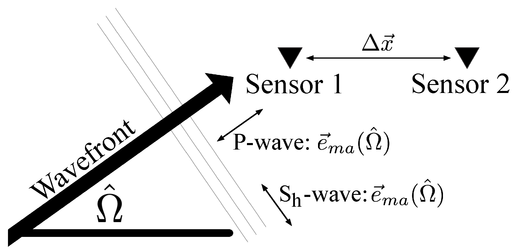
Abstract
:1. Introduction
2. Formalism
2.1. Body-Wave Formalism
2.2. Surface-Wave Formalism
2.3. Inversion Approach and Map Making
3. Performance Assessment
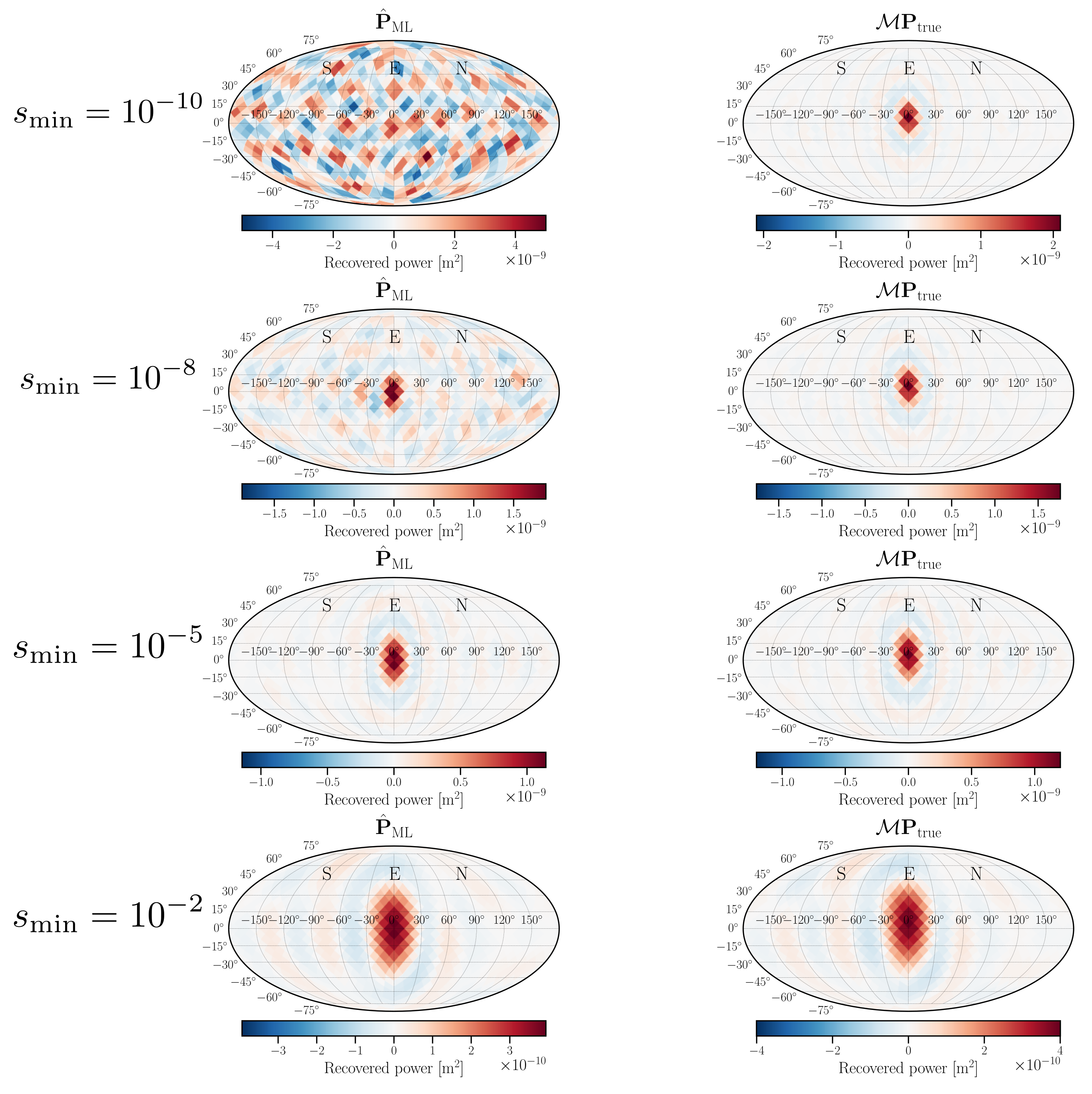
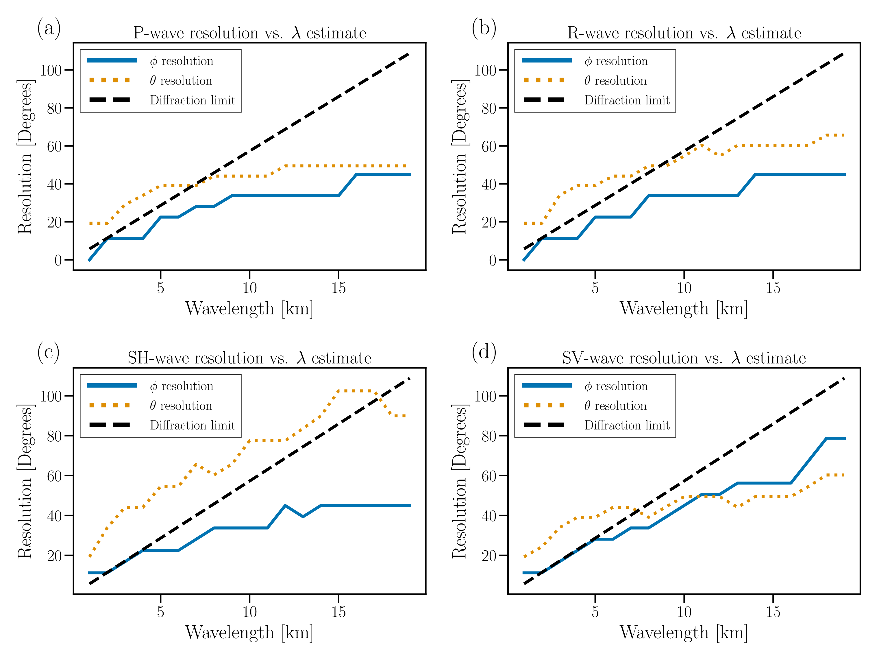
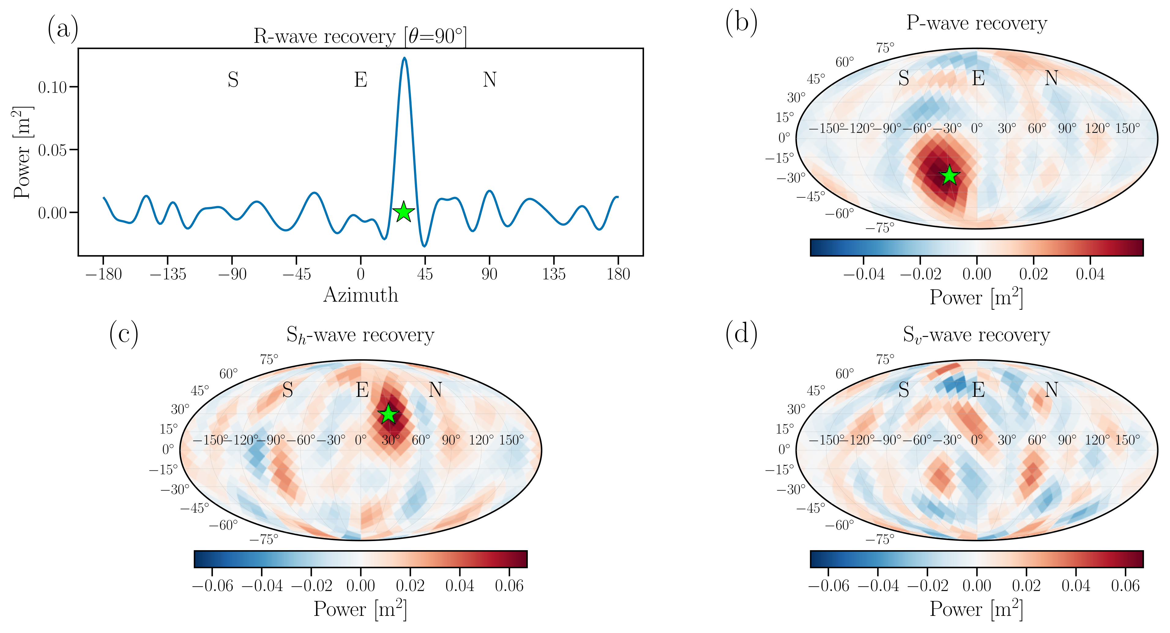
3.1. Performance Assessment Using Simulations
3.2. Performance Assessment Using Homestake Data
4. Microseism Noise Composition at Homestake
5. Conclusions
Supplementary Materials
Author Contributions
Funding
Data Availability Statement
Acknowledgments
Conflicts of Interest
References
- Gerstoft, P.; Tanimoto, T. A year of microseisms in southern California. Geophys. Res. Lett. 2007, 34, 2–7. [Google Scholar] [CrossRef] [Green Version]
- Kedar, S.; Longuet-Higgins, M.; Webb, F.; Graham, N.; Clayton, R.; Jones, C. The origin of deep ocean microseisms in the North Atlantic Ocean. Proc. R. Soc. A Math. Phys. Eng. Sci. 2008, 464, 777–793. [Google Scholar] [CrossRef]
- Ardhuin, F.; Herbers, T.H. Noise generation in the solid Earth, oceans and atmosphere, from nonlinear interacting surface gravity waves in finite depth. J. Fluid Mech. 2013, 716, 316–348. [Google Scholar] [CrossRef] [Green Version]
- Landés, M.; Hubans, F.; Shapiro, N.M.; Paul, A.; Campillo, M. Origin of deep ocean microseisms by using teleseismic body waves. J. Geophys. Res. Solid Earth 2010, 115, 1–14. [Google Scholar] [CrossRef] [Green Version]
- Juretzek, C.; Hadziioannou, C. Where do ocean microseisms come from? A study of Love-to-Rayleigh wave ratios. J. Geophys. Res. Solid Earth 2016, 121, 6741–6756. [Google Scholar] [CrossRef] [Green Version]
- Nishida, K.; Takagi, R. Teleseismic S Wave Microseisms. Science 2016, 353, 919–921. [Google Scholar] [CrossRef] [PubMed]
- Liu, Q.; Koper, K.D.; Burlacu, R.; Ni, S.; Wang, F.; Zou, C.; Wei, Y.; Gal, M.; Reading, A.M. Source locations of teleseismic P, SV, and SH waves observed in microseisms recorded by a large aperture seismic array in China. Earth Planet. Sci. Lett. 2016, 449, 39–47. [Google Scholar] [CrossRef]
- Ward Neale, J.; Harmon, N.; Srokosz, M. Improving Microseismic P Wave Source Location With Multiple Seismic Arrays. J. Geophys. Res. Solid Earth 2018, 123, 476–492. [Google Scholar] [CrossRef] [Green Version]
- Lobkis, O.I.; Weaver, R.L. On the emergence of the Green’s function in the correlations of a diffuse field. J. Acoust. Soc. Am. 2001, 110, 3011. [Google Scholar] [CrossRef] [Green Version]
- Shapiro, N.M.; Campillo, M.; Stehly, L.; Ritzwoller, M.H. High-resolution surface-wave tomography from ambient seismic noise. Science 2005, 307, 1615–1618. [Google Scholar] [CrossRef] [Green Version]
- Tsai, V.C. On establishing the accuracy of noise tomography travel-time measurements in a realistic medium. Geophys. J. Int. 2009, 178, 1555–1564. [Google Scholar] [CrossRef] [Green Version]
- Van Veen, B.D.; Buckley, K.M. Beamforming: A Versatile Approach to Spatial Filtering. IEEE ASSP Mag. 1988, 5, 4–24. [Google Scholar] [CrossRef]
- Rost, S.; Thomas, C. Array seismology: Methods and applications. Rev. Geophys. 2002, 40, 2-1–2-27. [Google Scholar] [CrossRef] [Green Version]
- Lehujeur, M.; Maggi, A.; Schmittbuhl, J. Ambient noise tomography with non-uniform noise sources and low aperture networks: Case study of deep geothermal reservoirs in northern Alsace, France. Geophys. J. Int. 2017, 208, 193–210. [Google Scholar] [CrossRef]
- Esmersoy, C.; Cormier, V.F.; Toksoz, M.N. Three-component array processing. VELA Program Twenty-Five Year Rev. Basic Res. 1985, 78, 1725–1743. [Google Scholar]
- Jurkevics, A. Polarization analysis of three-component array data. Bull. Seismol. Soc. Am. 1988, 78, 1725–1743. [Google Scholar]
- Wagner, G.S. Resolving diversely polarized, superimposed signals in three-component seismic array data. Geophys. Res. Lett. 1996, 23, 1837–1840. [Google Scholar] [CrossRef]
- Riahi, N.; Bokelmann, G.; Sala, P.; Saenger, E.H. Time-lapse analysis of ambient surface wave anisotropy: A three-component array study above an underground gas storage. J. Geophys. Res. Solid Earth 2013, 118, 5339–5351. [Google Scholar] [CrossRef]
- Löer, K.; Riahi, N.; Saenger, E.H. Three-component ambient noise beamforming in the Parkfield area. Geophys. J. Int. 2018, 213, 1478–1491. [Google Scholar] [CrossRef]
- Sánchez-Sesma, F.J.; Rodríguez, M.; Iturrarán-Viveros, U.; Luzón, F.; Campillo, M.; Margerin, L.; García-Jerez, A.; Suarez, M.; Santoyo, M.A.; Rodríguez-Castellanos, A. A theory for microtremor H/V spectral ratio: Application for a layered medium. Geophys. J. Int. 2011, 186, 221–225. [Google Scholar] [CrossRef] [Green Version]
- Bard, P.Y.; Bouchon, M. The seismic response of sediment-filled valleys. Part 2. The case of incident P and SV waves. Bull. Seismol. Soc. Am. 1980, 70, 1921–1941. [Google Scholar] [CrossRef]
- Bard, P.y.; Bouchon, M. The seismic response of sediment-filled valleys. Part 1. The case of incident SH waves. Bull. Seismol. Soc. Am. 1980, 70, 1263–1286. [Google Scholar] [CrossRef]
- Bowden, D.C.; Tsai, V.C. Earthquake ground motion amplification for surface waves. Geophys. Res. Lett. 2017, 43, 121–127. [Google Scholar] [CrossRef] [Green Version]
- Harms, J. Terrestrial gravity fluctuations. Living Rev. Relativ. 2019, 22, 6. [Google Scholar] [CrossRef] [Green Version]
- Baggeroer, A.B.; Kuperman, W.A.; Schmidt, H.; Baggeroer, A.B. Matched field processing: Source localization in correlated noise as an optimum parameter estimation problem. J. Acoust. Soc. Am. 1988, 83, 571–587. [Google Scholar] [CrossRef]
- Corciulo, M.; Roux, P.; Campillo, M.; Dubucq, D.; Kuperman, W.A. Multiscale matched-field processing for noise-source localization in exploration geophysics. Geophysics 2012, 77, KS33–KS41. [Google Scholar] [CrossRef]
- Gal, M.; Reading, A.M.; Rawlinson, N.; Schulte-Pelkum, V. Matched Field Processing of Three-Component Seismic Array Data Applied to Rayleigh and Love Microseisms. J. Geophys. Res. Solid Earth 2018, 123, 6871–6889. [Google Scholar] [CrossRef]
- Tromp, J.; Luo, Y.; Hanasoge, S.; Peter, D. Noise cross-correlation sensitivity kernels. Geophys. J. Int. 2010, 183, 791–819. [Google Scholar] [CrossRef] [Green Version]
- Sager, K.; Ermert, L.; Boehm, C.; Fichtner, A. Towards full waveform ambient noise inversion. Geophys. J. Int. 2018, 212, 566–590. [Google Scholar] [CrossRef]
- Sager, K.; Boehm, C.; Ermert, L.; Krischer, L.; Fichtner, A. Global-Scale Full-Waveform Ambient Noise Inversion. J. Geophys. Res. Solid Earth 2020, 125, 1–17. [Google Scholar] [CrossRef]
- Igel, J.K.H.; Ermert, L.A.; Fichtner, A. Rapid finite-frequency microseismic noise source inversion at regional to global scales. Geophys. J. Int. 2021, 227, 169–183. [Google Scholar] [CrossRef]
- Xu, Z.; Mikesell, T.D.; Gribler, G.; Mordret, A. Rayleigh-wave multicomponent cross-correlation-based source strength distribution inversion. Part 1: Theory and numerical examples. Geophys. J. Int. 2019, 218, 1761–1780. [Google Scholar] [CrossRef]
- Aki, K. Space and time spectra of stationary stochastic waves, with special reference to microtremors. Bull. Earthq. Res. Inst. 1957, 35, 415–457. [Google Scholar]
- Cox, H. Spatial correlation in arbitrary noise fields with application to ambient sea noise. J. Acoust. Soc. Am. 2010, 54, 1973. [Google Scholar] [CrossRef]
- Harmon, N.; Rychert, C.; Gerstoft, P. Distribution of noise sources for seismic interferometry. Geophys. J. Int. 2010, 183, 1470. [Google Scholar] [CrossRef] [Green Version]
- Haney, M.M.; Mikesell, T.D.; van Wijk, K.; Nakahara, H. Extension of the spatial autocorrelation (SPAC) method to mixed-component correlations of surface waves. Geophys. J. Int. 2012, 191, 189–206. [Google Scholar] [CrossRef] [Green Version]
- Ballmer, S.W. A radiometer for stochastic gravitational waves. Class. Quantum Gravity 2006, 23, S179. [Google Scholar] [CrossRef] [Green Version]
- Thrane, E.; Ballmer, S.; Romano, J.; Mitra, S.; Talukder, D.; Bose, S.; Mandic, V. Probing the anisotropies of a stochastic gravitational-wave background using a network of ground-based laser interferometers. Phys. Rev. D 2009, 80, 122002. [Google Scholar] [CrossRef] [Green Version]
- Romano, J.; Taylor, S.; Cornish, N.; Gair, J.; Mingarelli, C.; van Haasteren, R. Phase-coherent mapping of gravitational-wave backgrounds using ground-based laser interferometers. Phys. Rev. D 2015, 92, 042003. [Google Scholar] [CrossRef] [Green Version]
- Prestegard, T. Unmodeled Searches for Long-Lasting Gravitational-Wave Signals with LIGO and Studies of Underground Seismic Noise for Future Gravitational-Wave Detectors. Ph.D. Thesis, University of Minnesota, Minneapolis, MN, USA, 2016. [Google Scholar]
- Meyers, P. Cross-Correlation Searches for Persistent Gravitational Waves with Advanced LIGO and Noise Studies for Current and Future Ground-Based Gravitational-Wave Detectors. Ph.D. Thesis, University of Minnesota, Minneapolis, MN, USA, 2018. [Google Scholar]
- Park, S.; Ishii, M. Near-surface compressional and shear wave speeds constrained by body-wave polarization analysis. Geophys. J. Int. 2018, 213, 1559–1571. [Google Scholar] [CrossRef]
- Park, S.; Tsai, V.C.; Ishii, M. Frequency-dependent P wave polarization and its subwavelength near-surface depth sensitivity. Geophys. Res. Lett. 2019, 46, 14377–14384. [Google Scholar] [CrossRef]
- Haney, M.M.; Tsai, V.C. Nonperturbational surface-wave inversion: A Dix-type relation for surface waves. Geophysics 2015, 80, EN167–EN177. [Google Scholar] [CrossRef] [Green Version]
- Meyers, P.; Bowden, D.C.; Prestegard, T.; Tsai, V.C.; Mandic, V.; Pavlis, G.; Caton, R. Direct Observations of Surface-Wave Eigenfunctions at the Homestake 3D Array. Bull. Seismol. Soc. Am. 2019, 109, 1194–1202. [Google Scholar] [CrossRef]
- Paige, C.C.; Saunders, M.A. LSQR: An Algorithm for Sparse Linear Equations and Sparse Least Squares. ACM Trans. Math. Softw. 1982, 8, 43–71. [Google Scholar] [CrossRef]
- Hestenes, M.R.; Stiefel, E. Methods of Conjugate Gradients for Solving Linear Systems. J. Res. Natl. Bur. Stand. 1952, 49, 409–436. [Google Scholar] [CrossRef]
- Gorski, K.M.; Hivon, E.; Banday, A.J.; Wandelt, B.D.; Hansen, F.K.; Reinecke, M.; Bartelmann, M. HEALPix: A Framework for High-Resolution Discretization and Fast Analysis of Data Distributed on the Sphere. Astrophys. J. 2005, 622, 759–771. [Google Scholar] [CrossRef]
- Mandic, V.; Tsai, V.C.; Pavlis, G.L.; Prestegard, T.; Bowden, D.C.; Meyers, P.; Caton, R. A 3D Broadband Seismometer Array Experiment at the Homestake Mine. Seismol. Res. Lett. 2018, 89, 2420–2429. [Google Scholar] [CrossRef]
- Coughlin, M.; Harms, J.; Bowden, D.C.; Meyers, P.; Tsai, V.C.; Mandic, V.; Pavlis, G.; Prestegard, T. Coherence-Based Approaches for Estimating the Composition of the Seismic Wavefield. J. Geophys. Res. Solid Earth 2019, 124, 2941–2956. [Google Scholar] [CrossRef]
- Lovejoy, S. What Is Climate? Eos Trans. Am. Geophys. Union 2013, 94, 1–2. [Google Scholar] [CrossRef]
- Stehly, L.; Campillo, M.; Shapiro, N.M. A study of the seismic noise from its long-range correlation properties. J. Geophys. Res. Solid Earth 2006, 111. [Google Scholar] [CrossRef]
- Xu, Y.; Koper, K.D.; Burlacu, R. Lakes as a Source of Short-Period (0.5–2 s) Microseisms. J. Geophys. Res. Solid Earth 2017, 122, 8241–8256. [Google Scholar] [CrossRef]
- Bensen, G.D.; Ritzwoller, M.H.; Shapiro, N.M. Broadband ambient noise surface wave tomography across the United States. J. Geophys. Res. Solid Earth 2008, 113. [Google Scholar] [CrossRef] [Green Version]


Publisher’s Note: MDPI stays neutral with regard to jurisdictional claims in published maps and institutional affiliations. |
© 2021 by the authors. Licensee MDPI, Basel, Switzerland. This article is an open access article distributed under the terms and conditions of the Creative Commons Attribution (CC BY) license (https://creativecommons.org/licenses/by/4.0/).
Share and Cite
Meyers, P.M.; Prestegard, T.; Mandic, V.; Tsai, V.C.; Bowden, D.C.; Matas, A.; Pavlis, G.; Caton, R. A Linear Inversion Approach to Measuring the Composition and Directionality of the Seismic Noise Field. Remote Sens. 2021, 13, 3097. https://doi.org/10.3390/rs13163097
Meyers PM, Prestegard T, Mandic V, Tsai VC, Bowden DC, Matas A, Pavlis G, Caton R. A Linear Inversion Approach to Measuring the Composition and Directionality of the Seismic Noise Field. Remote Sensing. 2021; 13(16):3097. https://doi.org/10.3390/rs13163097
Chicago/Turabian StyleMeyers, Patrick M., Tanner Prestegard, Vuk Mandic, Victor C. Tsai, Daniel C. Bowden, Andrew Matas, Gary Pavlis, and Ross Caton. 2021. "A Linear Inversion Approach to Measuring the Composition and Directionality of the Seismic Noise Field" Remote Sensing 13, no. 16: 3097. https://doi.org/10.3390/rs13163097
APA StyleMeyers, P. M., Prestegard, T., Mandic, V., Tsai, V. C., Bowden, D. C., Matas, A., Pavlis, G., & Caton, R. (2021). A Linear Inversion Approach to Measuring the Composition and Directionality of the Seismic Noise Field. Remote Sensing, 13(16), 3097. https://doi.org/10.3390/rs13163097