Abstract
Polarimetric radar data (PRD) have potential to be used in numerical weather prediction (NWP) models to improve convective-scale weather forecasts. However, thus far only a few studies have been undertaken in this research direction. To assimilate PRD in NWP models, a forward operator, also called a PRD simulator, is needed to establish the relation between model physics parameters and polarimetric radar variables. Such a forward operator needs to be accurate enough to make quantitative comparisons between radar observations and model output feasible, and to be computationally efficient so that these observations can be easily incorporated into a data assimilation (DA) scheme. To address this concern, a set of parameterized PRD simulators for the horizontal reflectivity, differential reflectivity, specific differential phase, and cross-correlation coefficient were developed. In this study, we have tested the performance of these new operators in a variational DA system. Firstly, the tangent linear and adjoint (TL/AD) models for these PRD simulators have been developed and checked for the validity. Then, both the forward operator and its adjoint model have been built into the three-dimensional variational (3DVAR) system. Finally, some preliminary DA experiments have been performed with an idealized supercell storm. It is found that the assimilation of PRD, including differential reflectivity and specific differential phase, in addition to radar radial velocity and horizontal reflectivity, can enhance the accuracy of both initial conditions for model hydrometer state variables and ensuing model forecasts. The usefulness of the cross-correlation coefficient is very limited in terms of improving convective-scale data analysis and NWP.
1. Introduction
The accuracy of the initial conditions of numerical weather prediction (NWP) models has a great impact on their forecast results, especially for high-resolution NWP. To build up the initial hydrometeor information which is the key to successful simulating and forecasting of convective storms, the inevitable process known as “spin-up” is needed for NWP models [1]. In order to reduce the negative influence of “spin-up” on the forecast skill of short-lived convective storms, Doppler weather radar observations, including the horizontal reflectivity (ZH) and radial velocity (Vr), are commonly used to improve the initial condition with advanced data assimilation (DA) methods, such as the three-dimensional variational (3DVAR) method [2,3,4,5,6,7], the four-dimensional variational (4DVAR) method [8,9,10,11,12], and the ensemble Kalman filter (EnKF) [13,14,15,16,17,18].
The detection of additional measurements representing the microphysical characteristics of precipitation systems, such as the differential reflectivity (ZDR), cross-correlation coefficient (ρhv), and differential phase (ϕHV), which is the range integral of the specific differential phase (KDP), benefits from polarimetric radar technology that has been widely concerned and developed rapidly after decades of effort. Nowadays, polarimetric radars are deployed and applied globally; in the U.S., for instance, the national radar network of WSR-88D has been upgraded with dual-polarization capability, and polarimetric radar data (PRD) are available nationally [19,20]. The PRD has been also successfully used in quantitative precipitation estimation (QPE) [21,22,23,24], hydrometeor classification (HC) [25,26,27], microphysics retrieval [28,29,30,31] and severe weather identification [32,33,34,35]. These mentioned advantages prompt us to further explore the possibility of assimilating PRD into NWP models to improve weather forecasts, especially for the prediction of convective-scale weather.
A forward observation operator, also known as the PRD simulator, is needed to establish the relation between model state variables and PRD for their assimilation in NWP models. Many polarimetric radar rain estimators have been developed and used for QPE [21,29,30]. These relations have also been extended for ice phases including snow and ice [36,37]. Because of the complex nature and nonlinear interaction in mixed phases, these aforementioned single species estimators are unable to fully establish the relation between the multiple species of model state variables and PRD for DA use.
To use PRD in the DA process of improving the accuracy of the initial conditions, or obtain the simulated PRD from model microphysics state variables, Pfeifer et al. [38] and Jung et al. [39] (hereafter J08) developed their own PRD simulators, respectively. Both studies include the contribution of ice and melting species to polarimetric parameters, but the former considers the attenuation effect of radar beams as well, while the latter emphasizes the important influence of melting ice particles. Then, Jung et al. [40] first directly assimilated PRD using the ensemble square-root Kalman filter (EnSRF) with a single-moment (SM) microphysical parameterization (MP) scheme, and then attained the improved analysis of the storm when polarimetric variables were assimilated. Applying rigorous scattering calculations via the T-matrix method, a more accurate and numerically integrated observation operator was developed by Jung et al. [41] (hereafter J10). Compared the simulation performance of J10 under SM and double-moment (DM) MP schemes, Jung et al. [42] found that some realistic polarimetric signatures reported in observational studies such as ZDR arc, midlevel ZDR, and ρhv ring [23,33] can only be reproduced by employing a DM MP scheme.
Li and Mecikalski [43,44] used empirical relations and retrieved the rain water mixing ratio from ZDR [45] and KDP [46], respectively, and then assimilated them in the Weather Research and Forecasting (WRF) model using the WRF 3DVAR system. The consequences demonstrate the benefits of utilizing polarimetric variables to improve the initial condition and even short-term forecasts for mesoscale convective systems (MCSs). Then, Li et al. [47] developed an ice-phase operator embedded in the WRF 3DVAR system for assimilation of KDP, which can also additionally adjust solid water (cloud ice and snow) through DA. Consequently, a positive impact of extra KDP assimilation on analysis fields of rainwater in the lower troposphere and snow in the mid- to upper troposphere for an MCS was found. Aimed at applying J08 under the variational DA framework, Wang and Liu [48] rebuilt an operator named RadZIceVar (a package containing a reflectivity forward operator with its associated TL/AD operators together) and indicated its successful implement in DA use and significant improvement on short-term (2-5 h) precipitation forecast. However, the direct assimilation was applicable for ZH only, and assimilation of polarimetric variables was not supported.
Meanwhile, using J08 with SM and DM MP schemes, Putnam et al. [16] noted several microphysics biases with the help of simulated PRD through qualitative and quantitative verification of ensemble probabilistic forecasts in a real case. Subsequently, by establishing look-up tables to increase the calculation efficiency of J10 during the DA procedure, Putnam et al. [17] first implemented the direct assimilation of ZDR through the EnKF method for a real supercell case in the literature. Through a series of observing system simulation experiments (OSSEs) of an idealized supercell storm, Zhu et al. [18] investigated the impact of assimilating ZDR within an EnKF framework by using J10 coupled with a DM MP scheme, and also discussed the potential influence of updating hydrometeor number concentrations for DA effect. Their conclusions show that the assimilation of ZDR can improve the accuracy of analyzed hydrometeor fields in terms of pattern and intensity, and that updating the number concentrations with mixing ratios is important for deciding whether the benefit of assimilating ZDR can be preserved. However, they are all limited to the use of partial PRD for assimilation, and significant errors in the magnitude of analyzed PRD do exist, indicating that the operational application of PRD assimilation remains challenging.
In addition, some polarimetric signatures found in convective storms provide the opportunity for indirect assimilation of PRD. Using the Advanced Regional Prediction System (ARPS) cloud analysis module [5,49,50], Carlin et al. [51] managed to assimilate PRD through the detection of ZDR column signatures [33,52], which often occur in the strong updraft region within intense thunderstorms, to modify the temperature and moisture of the ARPS model. Encouraging results were obtained with improved analyses (more coherent updraft) and forecasts (more realistic reflectivity structures with better skill scores) compared to the original cloud analysis scheme without polarimetric information included. There are limits to the widespread use of this approach, however, due to the absence of ZDR columns in relatively weak precipitation systems and its high dependence on empirical relationships between model state variables and PRD.
Recently, Zhang et al. [53] (hereafter Z21) developed a new set of simplified and parameterized PRD observation operators which can link NWP model state variables and PRD for DA use, and verified its validity and applicability by applying an ideal case and a real case respectively. They found that the parameterized operators yield results consistent with that of rigorous calculation in J10. However, Z21 increased computational efficiency significantly, resulting in costs less than one percent of the computing time of J10 to complete the same task, which makes it more suitable for DA applications. Thus, in this study, the applicability of Z21 is investigated under a variational DA framework, and the different DA effects of each polarimetric variable are studied by conducting various OSSEs.
The rest of this paper is organized as follows. The new parameterized PRD operators are briefly reviewed in Section 2 and the overview of the 3DVAR DA system is provided in the following section. In Section 4, the experimental design is given, and some preliminary experiment results are discussed in Section 5. A summary and conclusions for this study are presented in the last section.
2. Polarimetric Radar Observation Operator
2.1. Microphysics Models and Parametrization
SM and DM MP schemes are commonly used in NWP models [54,55,56,57,58]. In SM simulations of NWP models, water mixing ratios (), which is directly relevant to water content (, where is the air density), is the only prognostic physics variable for hydrometeor physics. For DM MP schemes, the number concentration () and the water mixing ratio () are both predicted variables. For a given two-parameter drop/particle size distribution (DSD/PSD) model and a specified hydrometeor , both and can be converted to mass-weighted diameter () and water content (); then, many other related quantities such as DSD/PSD parameter, rainfall rate and reflectivity are calculated by these two state variables. The detailed description of the derivation can be found in Z21.
2.2. Parameterized PRD Operators
Polarimetric radar variables (ZH, ZDR, KDP, ρhv) are expressed by the integrals of DSD/PSD weighted by the scattering amplitudes [59,60]. The scattering amplitudes are normally calculated by the T-matrix method, and the integrals are calculated numerically for accurate results. This was done in J10. However, the complex integral form and resulting expensive computational cost make it not convenient for variational DA use, which usually needs the operators to be efficient and easy calculation of the derivative.
Mahale et al. [61] represented polarimetric variables as simple functions of water mixing ratio and mass/volume-weighted diameter in the polynomial form for rain. In the case of ice phases and mixtures such as dry/melting snow, hail, and graupel, the calculation and parameterization are more complicated than those of rain induced by the increased variability in density during the melting stage and irregular shape, as well as the orientation of the particles. For simplification, a simple function of the percentage of melting () as following is used in Z21 to calculate the particle density for the melting hydrometeor species x:
where (the same as J08), stands for the dry/pure state of ice hydrometeor corresponding to the melting state, and is the density of water. Except for the mean axis ratio and standard deviation of the canting angles, Z21 makes some adjustments to allow a larger dynamic range of ZDR and ρhv. The shape and orientation of hydrometer particles follow the modeling and representation documented in J08. Similar to rain, for a given ice or mixed phase species x, including snow, hail, graupel, and their melting parts, PRD variables are calculated for a set of at a given , and then parameterized as functions of as follows:
where the reflectivity factor is (, unit: mm). The fitting coefficients associated with are provided in Table 1 and Table 2 of Z21, and more detailed descriptions for calculations, assumptions, and result analysis can also be found there.

Table 1.
Results of test for Z21 TL/AD operators

Table 2.
List of experiments.
3. The 3DVAR DA System
To test the assimilation performance of Z21 in a variational DA scheme, in this study, a 3DVAR DA system designed especially for radar data assimilation at the convective scale is employed. This 3DVAR system was initially developed at the Center for Analysis and Prediction of Storms (CAPS) and subsequently refined at National Severe Storms Laboratory (NSSL). The standard 3DVAR cost function can be written as follows [3]:
The cost function defined above contains three terms on the right-hand side. The first term is the background term, which defines the departure of the analysis vector from the background vector weighted by the inverse of the NWP model background error covariance matrix , where the analysis vector contains the following variables: the three wind components (, , and ) and the mixing ratios of hydrometeors (rain water, snow, hail, graupel, cloud water, cloud ice). The background error covariance matrix is modeled by the product of a diagonal matrix of the standard deviation of the background error and a spatial recursive filter [3]. The standard deviations for the model variables are derived from the statistics of the Rapid Update Cycle (RUC) model’s 3 h forecasts over several years from 2001 to 2004 [62]. The second term is the observation term, which defines the departure of the analysis vector x from the observation vector , where is the forward operator which builds a “bridge” between the model state variables and observation data. In this study, the new PRD operators (Z21), which can use both the mixing ratio and the number concentration from a DM MP scheme, will be discussed later. In the second term, is called the observation error covariance matrix which includes both instruments and representativeness errors. The observation errors’ standard deviation for PRD variables (Vr, ZH, ZDR, KDP, and ρhv) is specified empirically as 2 m/s, 3 dBZ, 0.5 dB, 0.5 °/km, and 0.1 respectively. Finally, as the third term on the right-side, represents the dynamic or equation constraints. This term has proved to be very important, particularly for this convective-scale 3DVAR system. For example, the mass continuity equation imposed as a weak constraint is helpful in producing more suitable wind analysis [2,3].
Radar radial velocity Vr is regarded as a crucial variable in the DA procedure [3,4,10] because it provides important wind field information and dynamic characteristics of the precipitation event. In this 3DVAR DA system, the forward observation operator for radial velocity considering the effects of the Earth’s curvature is expressed as:
where and is radar beam height and distance, respectively, over and along the curving Earth’s surface, is the radial slant range, and is the radar azimuth angle. The 4/3-effective Earth radius mode is assumed to follow for the propagation of radar beams [59]. The effect of hydrometeor fall velocity is neglected here, and will be considered in the follow-up real data case study.
For PRD, after the calculations for each species available in specified MP scheme through Equations (2)–(5), the final variables for the pixel are obtained by summing the contributions from all species as follows:
For the 3DVAR method used here, considering the variations of observational spacing existing among different observations, multiple analysis passes are usually used to analyze different observation types with different filter scales. Indeed, applying multiple-pass with a recursive filter is proven superior to the common single-pass method theoretically [6,43]. Hence, in this study, each PRD variable is analyzed in a separate pass.
The new operators have been proved efficiently in PRD simulation and therefore particularly suitable for DA purposes (Z21), including both variational and ensemble DA. In such applications, the TL/AD operators, coupled with the forward operators, are required for the variational assimilation, which are not necessarily found in the EnKF [63]. As a consequence, complex operators such as those used in J10 are more applicable to be employed through the EnKF method for DA use. Despite this difficulty, due to the simple polynomial form of Z21, the programming of corresponding TL/AD operators is implemented smoothly according to the rules of adjoint code construction [64,65].
The AD operator is the transpose of the TL operator. Therefore, how well TL operator approximates the nonlinear forward operator determines how valid the gradient of the cost function is. Following [66], to verify the correctness of the TL operator, one can define a function R(a), given by
where and are forward, tangent linear operator respectively. The represents a random picked base state and represents a perturbation state. Here, R(a) is calculated over all points in the domain. According to the theory, if R(a) in Equation (12) is close to 1 for any small values of a (see Table 1), meaning that the TL operator approximates the nonlinear forward operator well. The test results of the TL operator are listed in Table 1, as a keeps decreasing from 1 to 1E-14, the R(a) values for all polarimetric variables (R_ZH, R_ZDR, R_KDP and R_ρhv) are approaching 1 uniformly and steadily in the case of double precision. However, when a goes down to an extra small value, the R(a) starts to increase, which is caused by the rounding error of the calculator floating-point arithmetic operation. The above outcomes enable us to conclude that the assimilation system with the Z21 integrated passes the validity test and that the subsequent experimental research can be carried out reasonably.
4. Experimental Design
As discussed previously, PRD shows potential for enhancing storm simulations in terms of intensity and structure and ensuing short-range forecasts [16,17,18,40,42,43,44,51]. However the forward operators used thus far are either too simple [43,44] or too complicated [39,41]. The recently proposed parameterized PRD operators in Z21 can be used in different microphysics schemes and are relatively efficient.
In this study, a fully compressible and non-hydrostatic Advanced Research Weather Research and Forecasting (WRF-ARW) model (version 3.7.1) is used in a three-dimensional space for a supercell storm simulation. The horizontal resolution is 1 km with 121 grid points in the east-west and north-south directions. Simultaneously, 51 stretched levels up to 20 km (50 hPa, approximately) above ground level (AGL) are chosen. Open boundary conditions for the lateral and Rayleigh damping for the top boundary are used in this idealized case. The whole integration of the WRF-ARW model for simulation is 3 hours.
A modified sounding from a classic supercell event that occurred on 20 May 1977 in Del City, Oklahoma is used to provide the environmental field of the storm. A thermal bubble with a potential temperature perturbation of 3 K is added in the truth field to initiate convection [14,67,68,69]. This warm bubble is centered at the location of (x = 90 km, y = 40 km, z = 1.5 km) and has a 10 km horizontal radius and 1.5 km vertical radius inside the model domain. The Milbrandt and Yau scheme [55], a DM MP scheme consisting of the predicted mixing ratios of six-class hydrometeors, such as cloud water (), cloud ice (), rain water (), snow (), hail (), and graupel (), and their corresponding number concentrations (, , , , , and , respectively), is applied in description of microphysical processes in the idealized case. The time step for the integration of the prognostic equations is set to be 3 seconds. The standard 1.5-order TKE closure scheme is chosen for the turbulence parameterization, and other configurations are the same as that of Ge et al. [67].
During the 3 h truth simulation, the cloud forms around 10 min, rain water appears at 15 min, ice hydrometeors are generated at 20 min, and a single convective storm develops in the first 30 min (not shown). The storm reaches its mature stage at 45 min, then starts to split, evolves and slightly weakens. At 2 hours into the model integration, the right-splitting cell tends to dominate, as indicated by a clear hook echo and strong updraft.
Figure 1 shows the cycled DA and forecast scheme employed in OSSEs. Based on the truth simulation with WRF, all polarimetric radar observations (Vr, ZH, ZDR, KDP, and ρhv) can be simulated and used in the iterations of 3DVAR analysis to update the model state variables (, , , and ). After the analysis step, a 5 min forecast procedure is performed and the result is the background field (, , , and ) as the input of the DA analysis step in the next cycle. Considering the mixing ratios of precipitation are too small at the early stage of storm initiation, the idealized data are generated after the 30 min of model integration. Two assumed S-band radars are located in the southeast and southwest corner, respectively, and are performed on the VCP11 scan mode of WSR-88D radar (14 tilts from 0.5° to 19.5°). Idealized PRD is derived from the truth simulation output using the forward operators in Equations (7)–(11).
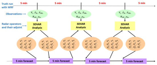
Figure 1.
Illustration of DA and forecast cycles used for the idealized case study. Observations represent the assimilated PRD including radar radial velocity, reflectivity, and all polarimetric variables simulated from the truth simulation output of the WRF run. The observations are assimilated by the 3DVAR system based on the background field of previous 5 min forecast result.
All OSSEs presented in this study are listed in Table 2. The control run assimilating Vr and ZH data, labeled as ExpVrZh, is considered as a reference for comparison purposes. Sensitivity experiments ExpVrZhZdr, ExpVrZhKdp, and ExpVrZhRhv are the same as the control run but with the additional assimilation of ZDR, KDP, and ρhv, respectively. ExpVrZhPol is a special run with all PRD assimilated. These sensitivity experiments are performed to help understand the impact of PRD on the analysis of hydrometer variables. Therein, the number concentrations of hydrometeors will not be updated during the DA cycles on account of the complexity introduced by their wide dynamic range (from 0 to above 1E12 m-3) and the problem of a significant increase of the degrees of freedom. The explanation of all abbreviations used in this paper can be found in Appendix A.
5. Results of 3DVAR Analysis
5.1. The Root Mean Square Error Analysis
The Root Mean Square Errors (RMSEs) are commonly used as a criterion for the accuracy judgment of DA [14,18,40,68,69]. To be consistent with the previous requirement of ZH assimilation, the RMSEs of analysis and forecast displayed in Figure 2 are only calculated over precipitation grids with ZH exceeding 10 dBZ.
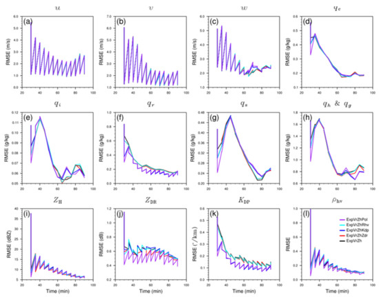
Figure 2.
The mean RMSEs of the forecasts and analyses throughout the 5 min 3DVAR DA cycles for ExpVrZh (black line), ExpVrZhZdr (red line), ExpVrZhKdp (blue line), ExpVrZhRhv (cyan line), and ExpVrZhPol (purple line), respectively, averaged over grid points where the observed (simulated) ZH is greater than 10 dBZ. (a) , (b) , (c) , mixing ratios of (d) cloud water , (e) cloud ice , (f) rain water , (g) snow , (h) hail , and graupel , and the same calculating procedure as truth simulations for polarimetric radar variables (i) ZH, (j) ZDR, (k) KDP, and (l) ρhv via Z21 forward operators.
At a first glance of Figure 2, for all model state variables and simulated radar observations, the RMSEs of analysis and forecast have a generally decreasing tendency over time for each OSSE. Since number concentrations are not updated with mixing ratios during the DA process, there may be a potential imbalance between them, leading to fluctuations in the early DA stages. Compared to ExpVrZh (black line), ExpVrZhZdr (red line) produces slightly better analyses and forecasts for most variables, where more pronounced improvements occur in the last few cycles, especially in ice hydrometeor species (Figure 2e), , and (Figure 2h). Since KDP is most sensitive to the presence of liquid water, the RMSE of (Figure 2f) of ExpVrZhKdp (blue line) has the most obvious difference. The better convergence through the whole DA cycle suggests that the satisfied rain water field much closer to the truth can be analyzed with additional KDP assimilation. In fact, as with ExpVrZhZdr, it also plays a positive role in obtaining a smaller RMSE in the last few cycles for , , and . For ExpVrZhRhv (cyan line), the relatively distinct variations only occur in the first or last few cycles, but as a whole, its RMSEs almost follow that of ExpVrZh with no significant discrepancies, indicating the limited effect of ρhv assimilation.
In terms of observed radar variables, the RMSEs of ExpVrZhZdr converge better and faster, indicating its simulated PRD is superior to that of ExpVrZh, especially for ZDR (Figure 2j) and ZH (Figure 2i). The above conclusions agree well with those of Jung et al. [40], except for benefits shown earlier in DA cycles here. This is largely the same as the result of Zhu et al. [18]. Apparently, ExpVrZhKdp produces consistently better KDP (Figure 2k) in both analysis and forecast cycles, as expected. Moreover, there are some subtle advancements of ZH in the last few cycles, but no contributions to the simulation of ZDR and ρhv (Figure 2l). As confirmed by the variation of the RMSEs, the assimilation of ρhv cannot bring benefits in observation space as well. Although both ZH and ρhv can converge reasonably, the influence of ρhv assimilation is too small to be noticed, which may be caused by the relatively small variation range of itself (on the order of 0.01). Noted that the reverse changing problem (the RMSE decreases in the forecast cycle, but increases in the corresponding analysis cycle) occurring in ZDR and KDP can be resolved by assimilating the corresponding PRD variable.
In the aspect of RMSEs, different abilities and effects in improving the accuracy of the model state variables and simulation of PRD have been presented for each polarimetric variable. Superior and more balanced results are expected to be achieved by jointly assimilating all PRD. As shown in purple line in Figure 2, although some fluctuations arise in (Figure 2c), (Figure 2g), and at certain cycles, the best convergent trends are obtained in ExpVrZhPol for almost all kinds of hydrometeors, especially in later DA cycles. For simulated PRD, ExpVrZhPol also acquires better RMSE convergence compared to other experiments, especially for ZDR and ρhv. Actually, with respect to most variables, the sharpest downward variation range occurring in the first cycle of ExpVrZhPol indirectly reveals the greatest potential capability of revising the model analysis field.
5.2. Evaluation of PRD Assimilation
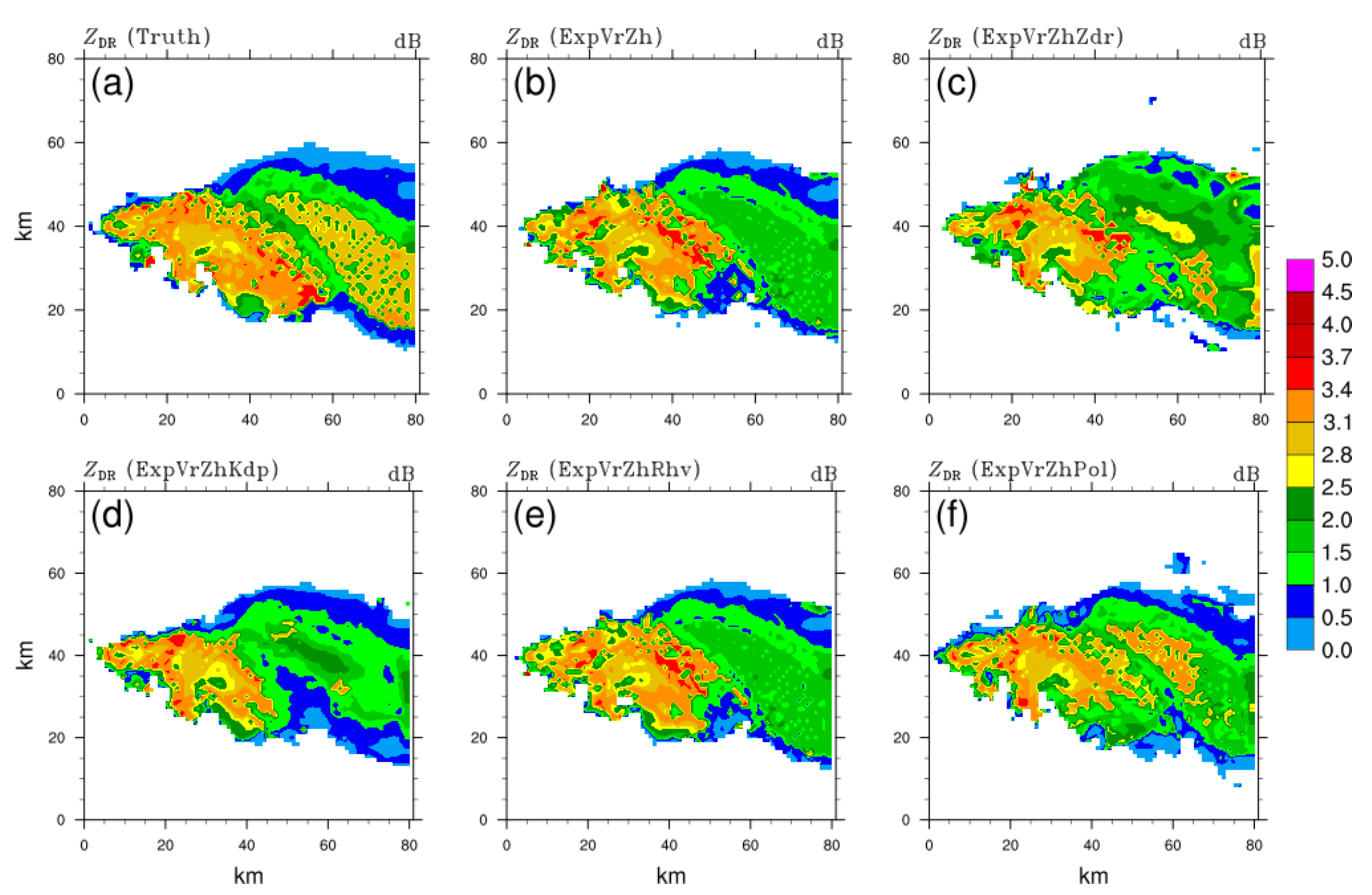
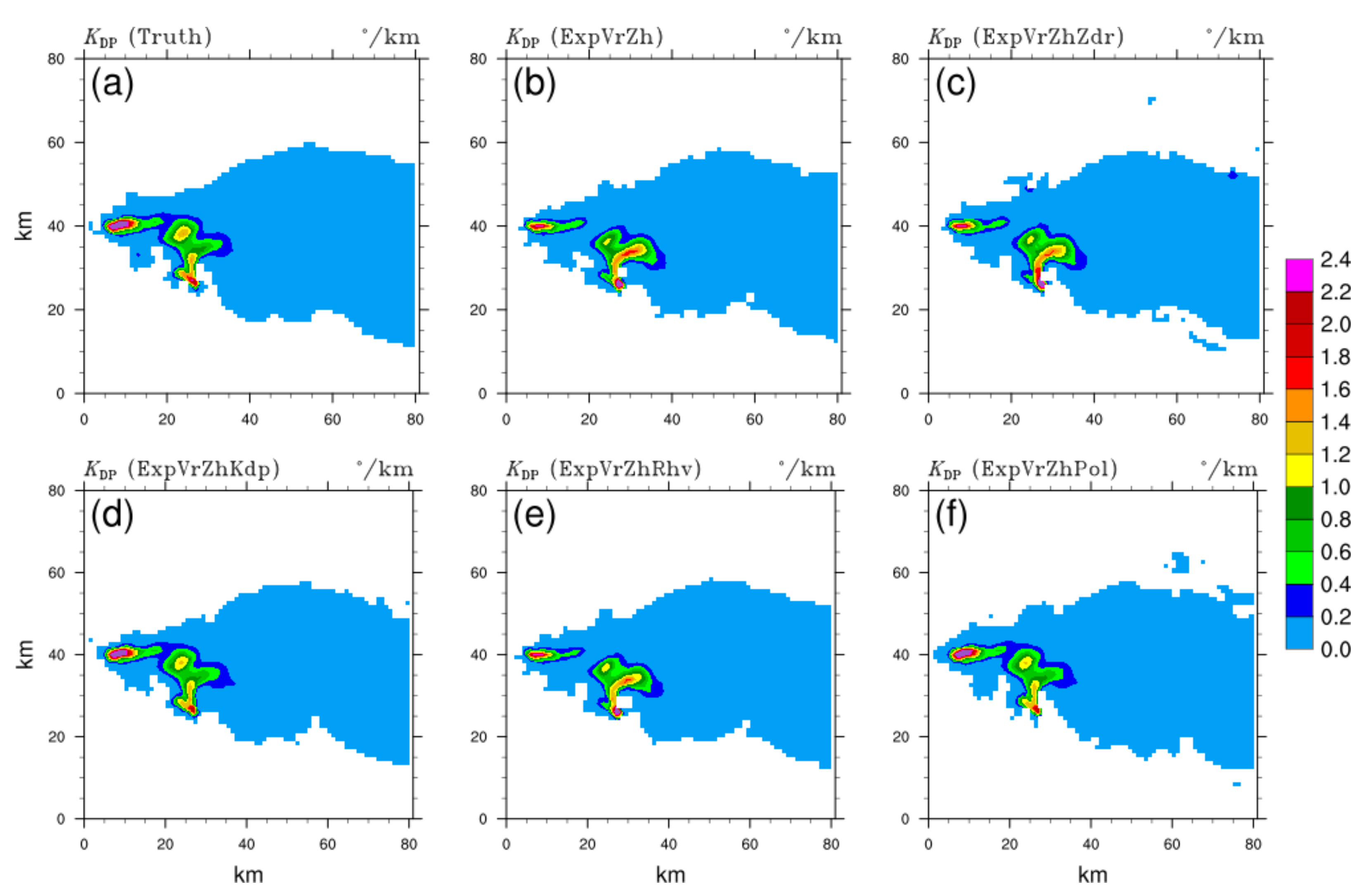
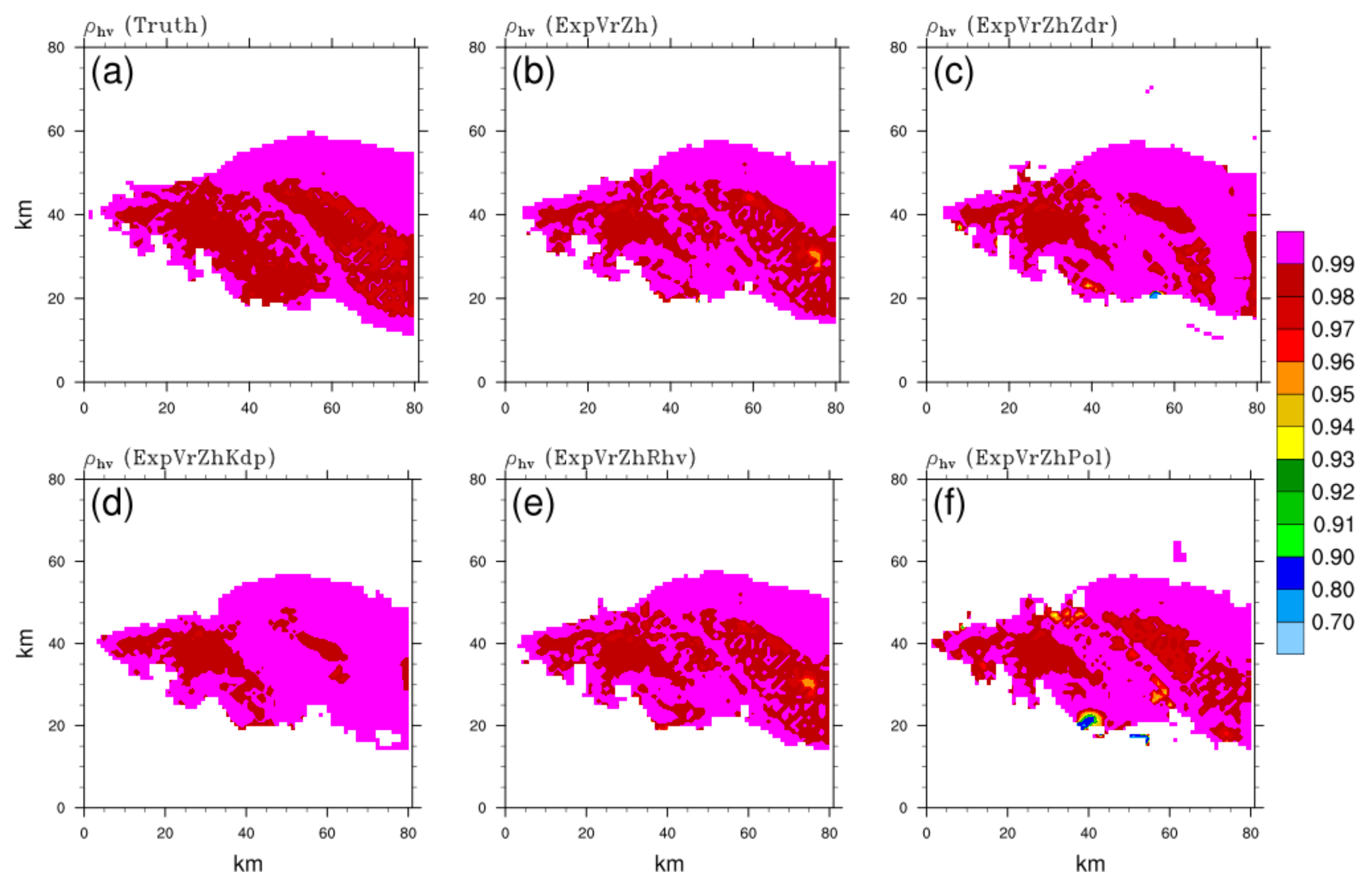
The impacts of PRD assimilation on the horizontal distribution of intensity and polarimetric characteristics of the simulated storm are further analyzed in Figure 3, Figure 4, Figure 5 and Figure 6. Compared with the true ZH (Figure 3a), all OSSEs represent the hook echo signature and the strong ZH core at the leading edge of the storm. Among them, ExpVrZh (Figure 3b) and ExpVrZhRhv (Figure 3e) have very similar results with obviously high ZH (greater than 15 dBZ overestimated) in the rear stratiform precipitation area (hereafter SPA). However, the ZH intensity described by ExpVrZhZdr (Figure 3c) is superior to them, both in the front convective precipitation area (CPA) and the rear SPA. However, the weak echo (<20 dBZ) on the northern edge is over-adjusted to deviate from the truth. On the contrary, although the weak echo is well analyzed, a much smaller ZH exists in the SPA of ExpVrZhKdp (Figure 3d). In terms of intensity and structure, the overall result of ExpVrZhPol (Figure 3f) is much closer to the truth, particularly in the echo edge and rear SPA, except for a certain overestimation in the CPA. There is a small ZDR patch (<1 dB) in the southeast corner of the main storm in ExpVrZh (Figure 4b), and also the same in ExpVrZhRhv (Figure 4e). Beyond that, the ZDR in the SPA is significantly smaller than the truth (Figure 4a), with the largest difference over 1.5 dB. ExpVrZhKdp (Figure 4d) has even worse simulation with much smaller ZDR. However, the intensity of ZDR in ExpVrZhZdr (Figure 4c) is much enhanced in the fore-mentioned two underestimated areas, particularly in the SPA. However, to some extent, overestimation persists in the weak echo at the edge of storm. ExpVrZhPol (Figure 4f) equally gives the best analysis among all OSSEs, except for the underestimation that occurred in the south-east of the storm. Although the dominant distribution of KDP is well exhibited in ExpVrZh (Figure 5b), ExpVrZhZdr (Figure 5c) and ExpVrZhRhv (Figure 5e) without KDP assimilation, the central strength of the leading edge and the hook echo are clearly weaker. The assimilation of KDP is beneficial that the simulated KDP shown in Figure 5d is perfectly matched with the truth (Figure 5a) in both intensity and structure. Undoubtedly, as a result of additional assimilation of KDP, ExpVrZhPol (Figure 5f) also has a similar good performance to ExpVrZhKdp. Based on the simulated result of ExpVrZh (Figure 6b) which is pretty close to the true ρhv (Figure 6a), ExpVrZhRhv (Figure 6e) mainly brings improvement in details, whereas ExpVrZhZdr (Figure 6c) and ExpVrZhKdp (Figure 6d) make further overestimation of ρhv in certain areas. Affected by ZDR and KDP, ExpVrZhPol (Figure 6f) does not exhibit better ρhv distribution, but instead has an underestimated area (<0.9).
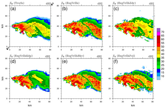
Figure 3.
The reflectivity ZH (unit: dBZ) at 1 km altitude at 80 min for (a) truth, and analysis fields of (b) ExpVrZh, (c) ExpVrZhZdr, (d) ExpVrZhKdp, (e) ExpVrZhRhv, and (f) ExpVrZhPol, respectively. The two assumed radars are located at the bottom-left and top-right corners as shown in Figure 3a.

Figure 4.
The same as Figure 3, but for the differential reflectivity ZDR (unit: dB) of (a) truth, and analysis fields of (b) ExpVrZh, (c) ExpVrZhZdr, (d) ExpVrZhKdp, (e) ExpVrZhRhv, and (f) ExpVrZhPol, respectively.

Figure 5.
The same as Figure 3, but for the specific differential phase KDP (unit: °/km) of (a) truth, and analysis fields of (b) ExpVrZh, (c) ExpVrZhZdr, (d) ExpVrZhKdp, (e) ExpVrZhRhv, and (f) ExpVrZhPol, respectively.

Figure 6.
The same as Figure 3, but for the cross-correlation coefficient ρhv (dimensionless) of (a) truth, and analysis fields of (b) ExpVrZh, (c) ExpVrZhZdr, (d) ExpVrZhKdp, (e) ExpVrZhRhv, and (f) ExpVrZhPol, respectively.
To further evaluate the simulation of the vertical structure of the storm in different DA schemes, the vertical slices of analyses through the intensity core and hook echo region (black dashed line in Figure 3a) are shown in Figure 7, Figure 8, Figure 9 and Figure 10. For ZH, the whole structure and extended height of the strong echo are both close to the truth (Figure 7a), with the exceptions of the ring-shape core (>55 dBZ) in ExpVrZh (Figure 7b), ExpVrZhZdr (Figure 7c), and ExpVrZhRhv (Figure 7e). Additionally, ZH in these OSSEs are overestimated markedly in the middle level of the forward flank (5 km horizontally, the same hereafter), which is reduced properly in ExpVrZhKdp (Figure 7d). Additionally, the overestimation in the low level of the rear SPA (30~40 km) has been alleviated by assimilating ZDR, such that the intensity is much closer to the truth and the echo goes from ungrounded to grounded. ExpVrZhRhv shows no enhancement compared with ExpVrZh, or even worse results (overestimation in some areas, Figure 7e vs. Figure 7a and Figure 7b). More than that, the ahead-developing convective cell (~6 km) and inner strong echo of the main storm are both better described in ExpVrZhKdp and ExpVrZhPol (Figure 7f). In comparison with the truth (Figure 8a), the signature of the ZDR column (~5 km) related to the updraft within the storm is more evidently discerned in ExpVrZdr (Figure 8c) and ExpVrKdp (Figure 8d), whereas the sagged high ZDR area (~25 km) attributed to the existence of a small number of large raindrops is well retained in ExpVrZh (Figure 8b), ExpVrZdr, and ExpVrRhv (Figure 8e). Modifications of amplitude and shape of ZDR can be noticed in the tail (~35 km) in ExpVrZhZdr and ExpVrZhKdp. With respect to above features, the best analysis result in terms of intensity and structure is given in ExpVrZhPol (Figure 8f). ExpVrZhKdp reveals an extremely high degree of similarity with the truth (Figure 9d vs. Figure 9a), including the KDP core associated with high liquid water content (LWC) within the storm, an overshooting structure linked to the strong updraft rushing through the melting layer, and even the small KDP area hanging ahead. The effect of KDP assimilation is maintained in ExpVrZhPol (Figure 9f), showing almost identical distribution characteristics to that of ExpVrZhKdp. Comparatively, other OSSEs (Figure 9b,c,e) nearly fail to reproduce these mentioned signatures. The melting layer associated with the melting hydrometeors is precisely described by a ρhv drop in these OSSEs, but with a wider melting band and a few underestimated areas above. Other than a small positive contribution from the ρhv assimilation (Figure 10e) in the low-value area located in the middle level of the forward edge (~5 km) of the storm, there are no notable improvements in the distribution of analyzed ρhv for different OSSEs.
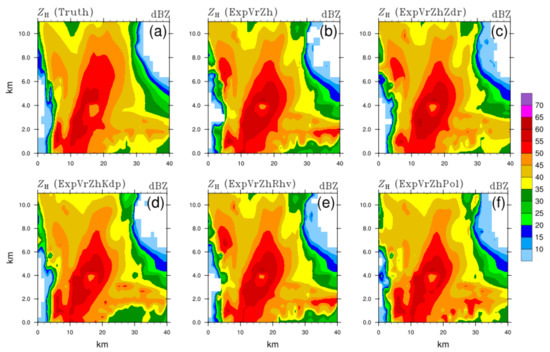
Figure 7.
Vertical cross-sections of reflectivity ZH along the black dashed line in Figure 3a for (a) truth, and analysis fields of (b) ExpVrZh, (c) ExpVrZhZdr, (d) ExpVrZhKdp, (e) ExpVrZhRhv, and (f) ExpVrZhPol, respectively.
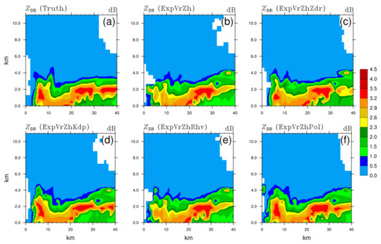
Figure 8.
The same as Figure 7, but for the differential reflectivity ZDR of (a) truth, and analysis fields of (b) ExpVrZh, (c) ExpVrZhZdr, (d) ExpVrZhKdp, (e) ExpVrZhRhv, and (f) ExpVrZhPol, respectively.
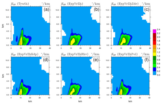
Figure 9.
The same as Figure 7, but for the specific differential phase KDP of (a) truth, and analysis fields of (b) ExpVrZh, (c) ExpVrZhZdr, (d) ExpVrZhKdp, (e) ExpVrZhRhv, and (f) ExpVrZhPol, respectively.
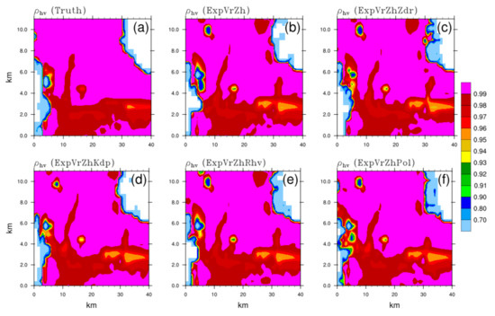
Figure 10.
The same as Figure 7, but for the cross-correlation coefficient ρhv of (a) truth, and analysis fields of (b) ExpVrZh, (c) ExpVrZhZdr, (d) ExpVrZhKdp, (e) ExpVrZhRhv, and (f) ExpVrZhPol, respectively.
5.3. Evaluation of Hydrometeor Analysis
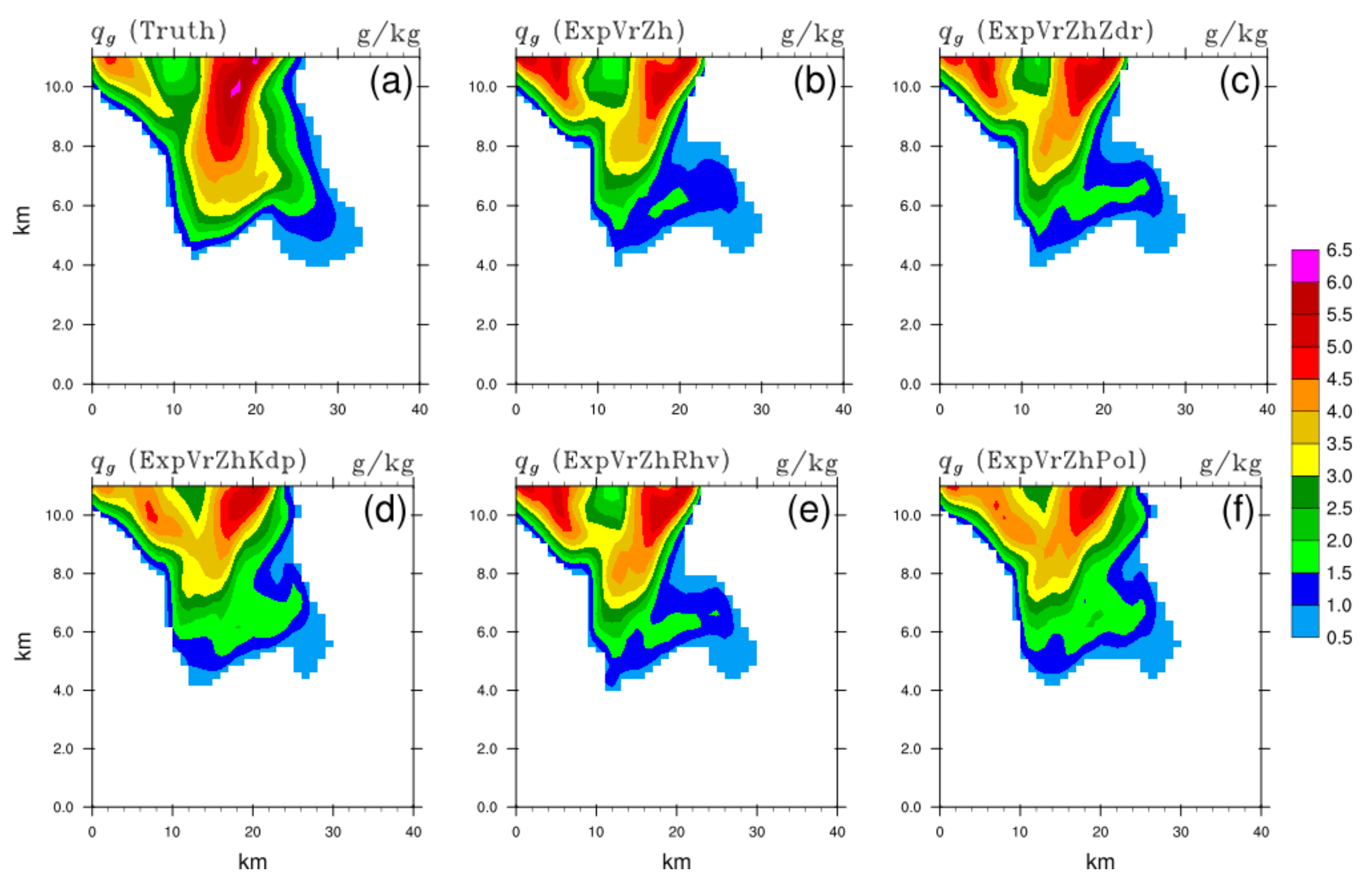
Figure 11, Figure 12, Figure 13 and Figure 14 show the mixing ratios of cloud ice , rain water , hail , and graupel in the truth and analysis fields of OSSEs, respectively, through identical vertical slices as in Figure 7. These OSSEs with PRD assimilation partially (mainly in the right part) and slightly (within 0.1 g/kg) strengthen more than that in ExpVrZh (Figure 11b), which is still much weaker compared to the truth (Figure 11a). Besides the basic distribution of , well depicted in OSSEs, the outstretched structure corresponding to the convection initiation ahead (~5 km) is better analyzed in ExpVrZhZdr (Figure 12c) and ExpVrZhKdp (Figure 12d). The latter better portrays the rear (>30 km) relatively small (0.1~0.2 g/kg), while the former is slightly over-adjusted (>0.2 g/kg). The overshooting pattern (~10 km) resulting from the strong updraft within the storm and suggesting the presence of super-cooled water is clearly displayed in ExpVrZhKdp as well, completely consistent with the truth (Figure 12a). However, the more obvious (Figure 13c) core (>1.8 g/kg) and enhanced (Figure 14c) in the middle- (>1.5 g/kg) and upper level (>4.0 g/kg) can be seen in ExpVrZhZdr. As expected, these mentioned benefits induced by ZDR or KDP assimilation are also retained in ExpVrZhPol. In addition, there are many other improvements such as the preferable descriptions of relatively small (<0.2 g/kg), (<0.6 g/kg), and (<4.5 g/kg) in the upper left corner f, Figure 13f and Figure 14f), the superior analysis much closer to the truth (Figure 12f vs. Figure 12a), and so on. However, apart from minor differences, all analyzed mixing ratios in ExpVrZhRhv are largely the same as the corresponding ones in ExpVrZh (Figure 11e, Figure 12e, Figure 13e and Figure 14e vs. Figure 11b, Figure 12b, Figure 13b and Figure 14b, respectively). Additionally, analyses of cloud water and snow yield similar results as other hydrometeor variables, that is, is similar to , and is similar to other ice species (, , and ), which are not detailed here.
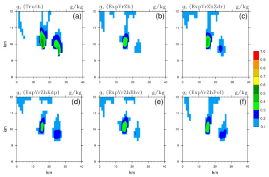
Figure 11.
The same as Figure 7, but for the mixing ratio of cloud ice (unit: g/kg) of (a) truth, and analysis fields of (b) ExpVrZh, (c) ExpVrZhZdr, (d) ExpVrZhKdp, (e) ExpVrZhRhv, and (f) ExpVrZhPol, respectively.
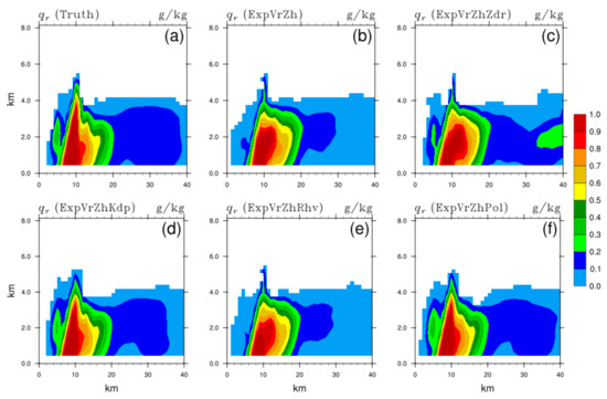
Figure 12.
The same as Figure 7, but for the mixing ratio of rain water (unit: g/kg) of (a) truth, and analysis fields of (b) ExpVrZh, (c) ExpVrZhZdr, (d) ExpVrZhKdp, (e) ExpVrZhRhv, and (f) ExpVrZhPol, respectively.
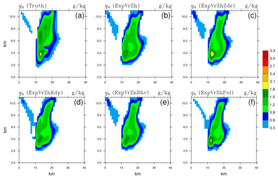
Figure 13.
The same as Figure 7, but for the mixing ratio of hail (unit: g/kg) of (a) truth, and analysis fields of (b) ExpVrZh, (c) ExpVrZhZdr, (d) ExpVrZhKdp, (e) ExpVrZhRhv, and (f) ExpVrZhPol, respectively.

Figure 14.
The same as Figure 7, but for the mixing ratio of graupel (unit: g/kg) of (a) truth, and analysis fields of (b) ExpVrZh, (c) ExpVrZhZdr, (d) ExpVrZhKdp, (e) ExpVrZhRhv, and (f) ExpVrZhPol, respectively.
In general, the above results further demonstrate the potential positive effects of ZDR assimilation on the analysis of solid hydrometeor particles, more benefits of KDP assimilation in improving the simulation of rain water rather than ice hydrometeors, and the limited usefulness of ρhv in terms of enhancing model hydrometeor analysis. Attributing to the combined positive impacts from PRD assimilations, more comprehensive hydrometeor analysis results in both intensity and pattern can be obtained. The conclusions are also in accordance with the findings of RMSE analysis.
Different PRD variables have different information contents and error effects corresponding to each hydrometeor. ZDR increases as the raindrop size increases or ice particles melt. Therefore, assimilation of ZDR yields improved analysis of all hydrometeors. KDP depends on both the raindrop size and the number concentration, hence, its assimilation improves the analysis of . Since ρhv reduction occurs only in the melting/mixing regions which have a very small percentage of the storm and it has a small dynamic range with relatively large errors, the improvement with assimilation of ρhv is minimal.
5.4. Evaluation of Forecast
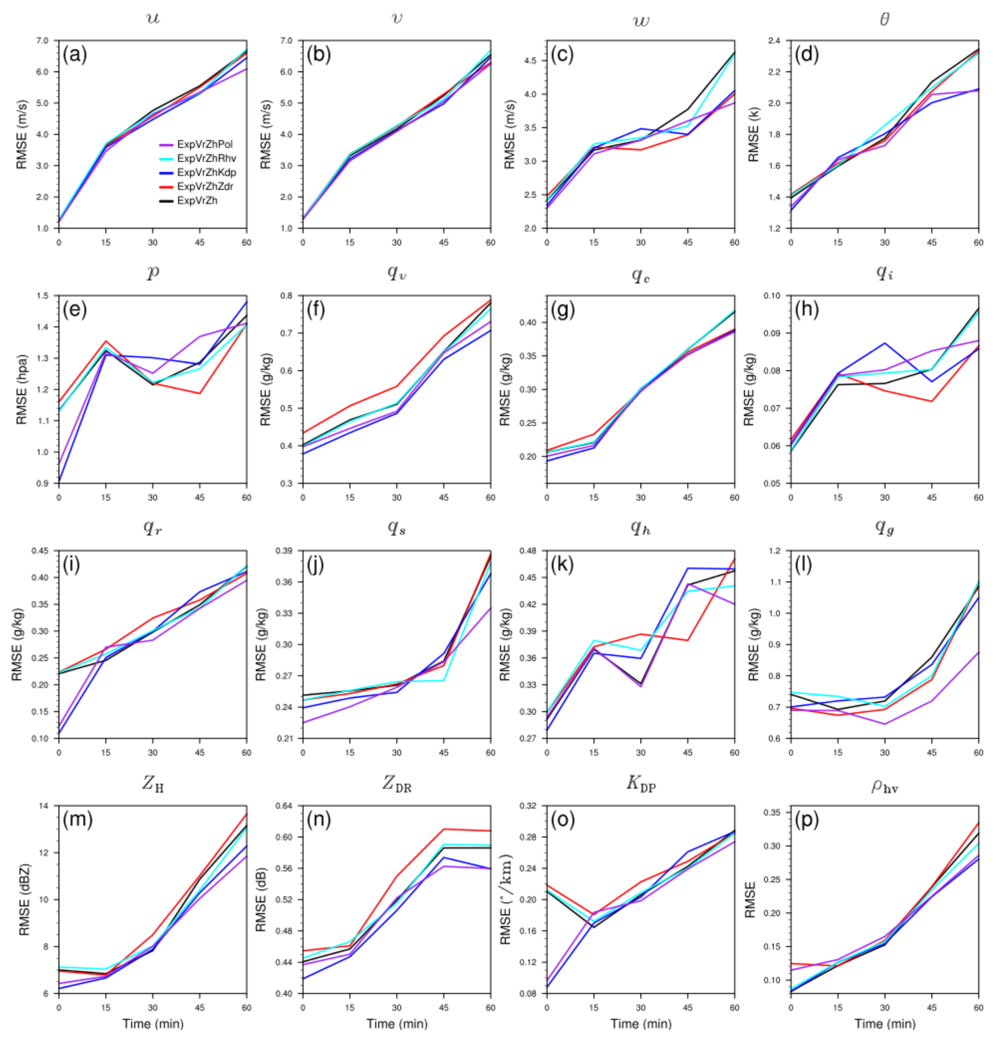
To investigate the improvement effect of modified initial conditions from different DA schemes on model predictions, the 1 h forecasts beginning at the 120 min of a storm are made at 15 min intervals for these OSSEs. In addition, the mean RMSEs of forecasts are calculated as seen in Figure 2 and displayed in Figure 15. Unsurprisingly, the increasing trend of RMSE with time is exhibited in all model state variables and simulated PRD, but the variation characteristics for different OSSEs are still existing diversely.
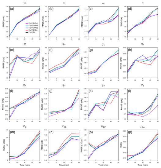
Figure 15.
The mean RMSEs of 1 h forecasts at a 15 min intervals initiated at 120 min for ExpVrZh (black line), ExpVrZhZdr (red line), ExpVrZhKdp (blue line), ExpVrZhRhv (cyan line), and ExpVrZhPol (purple line), respectively, averaged over grid points with observed (simulated) ZH exceeding 10 dBZ. (a) , (b) , (c) , (d) perturbation potential temperature , (e) perturbation pressure , mixing ratios of (f) water vapor , (g) cloud water , (h) cloud ice , (i) rain water , (j) snow , (k) hail , and (l) graupel , and simulated PRD in observation space: (m) ZH, (n) ZDR, (o) KDP, and (p) ρhv.
Taking all parameters into account, ExpVrZhPol (purple line) generally outperforms other OSSEs. Although the differences in the horizontal wind of and (Figure 15a,b) are almost indistinguishable, it can be seen upon careful inspection that ExpVrZhPol has a relatively low RMSE on the whole. Furthermore, except for the better performance of ExpVrZhZdr (red line) in the intermediate stage (30-45 min) of prediction, ExpVrZhPol also has the best overall prediction effect on vertical velocity (Figure 15c). An analogous situation appears in the perturbation potential temperature (Figure 15d) and perturbation pressure (Figure 15e) as well. For hydrometeors, the remarkable advancements resulting from combined assimilation of PRD can be found in cloud water (Figure 15g), rain water (Figure 15i), snow (Figure 15j), and graupel (Figure 15l) almost throughout the entire prediction period, and mainly in both ends of the period for cloud ice (Figure 15h) and hail (Figure 15k). While taken individually, with respect to RMSEs, ExpVrZhZdr has a good performance in ice hydrometeors (, , and ) forecasts, suggesting the potential advantages of ZDR assimilation in increasing the prediction accuracy of ice species. Further, due to the high sensitivity of KDP to liquid water, ExpVrZhKdp (blue line) illustrates more superiorities in the forecasting of water vapor (Figure 15f), , and . Comparatively speaking, ExpVrZhRhv (cyan line) has fully comparable behaviors with ExpVrZh (black line), demonstrating the limited benefits of ρhv assimilation.
In observation space, ExpVrZhPol also manifests superior overall performance, thoroughly in ZH (Figure 15m), and mainly in the late forecast stage (after 30 min) of ZDR (Figure 15n), KDP (Figure 15o) and ρhv (Figure 15p), which is of great significance for quantitative applications of PRD (precipitation estimation, hydrometeor classification, and so on). By contrast, ExpVrZhKdp is the second choice, having a suboptimal effect comprehensively. It is noteworthy that the RMSEs of ExpVrZhRhv nearly coincide with that of ExpVrZh for all PRD variables, further indicating the minor positive impact of ρhv assimilation on the forecasts.
6. Summary and Conclusions
In this paper, based on the new simplified and parameterized polarimetric radar observation operators developed by Z21, the corresponding TL/AD operators necessarily required by the variational DA procedure are constructed. The gradient check of the cost function in the minimization step of analysis cycles proves the operators work reasonably. In fact, as mentioned previously, the updating of number concentrations which affect the DA effect [18] is not considered here and is worthy of further research.
To evaluate the influences of assimilating the differential reflectivity ZDR, specific differential phase KDP, cross-correlation coefficient ρhv, as well as horizontal reflectivity ZH and radial velocity Vr, cycled 3DVAR DA and forecast schemes are performed. The truth is generated with a 3 h simulation of an idealized supercell storm using the WRF model. The PRD is constructed from the idealized truth simulations via Z21 forward operators. Then, these observations are assimilated into the WRF model at a 5 min interval with the initial DA beginning at 30 min of model integration.
Using the experiment of assimilating both ZH and Vr as the benchmark run, OSSEs with additional assimilation of ZDR, KDP, and ρhv, respectively, are performed to examine the impact of each polarimetric variable on DA results. Additionally, an extra OSSE which assimilates all PRD is conducted to see whether a more balanced result can be achieved. The results suggest that the ZDR assimilation adjusts all model state variables to varying degrees, and helps reduce RMSEs at almost each DA cycle. Moreover, the assimilation process makes some polarimetric signatures, such as hook echo, ZDR column and melting layer, more obvious, and improves the distributions of hydrometeors and observations much closer to the truth as well. High sensitivity to liquid water of KDP is believed to be responsible for the more improved analysis of rainwater, and the intensity and pattern of PRD are also enhanced with additional assimilation of KDP, especially for ZH and KDP itself. The small discrepancy between OSSEs with and without ρhv assimilation indicates its limited ability in adjusting model state variables and improving the analysis accuracy. In contrast, due to the accumulation of favorable DA effects of different polarimetric variables, assimilating all PRD obtains more balanced analysis results, as expected. The above polarimetric signatures are also well presented in observation space, and many other improvements have been made, including the optimization of rain water analysis which is perfectly matched with the reference truth, and better descriptions of some small value areas in mixing ratios of cloud water, snow, and graupel. These different assimilation results are attributed to the different information contents and error effects from PRD variables. It is noted that these characteristics of assimilation PRD can change depending on the type of storm and model microphysics as well as observation errors, which needs further study. A series of prediction experiments, which initiate at the 120 min of different OSSEs and run over a 1 h period at a 15 min interval, are conducted to further study the impact of improved initial conditions on ensuing forecasts. The RMSEs of forecasts are calculated and the results show that the ZDR assimilation can bring obvious benefits for forecasts of ice hydrometeor species including cloud ice, hail, and graupel and even for the vertical wind field and perturbation pressure in the late stage of prediction. Assimilating KDP is found to improve the prediction of water vapor, cloud water, and rainwater, which is consistent with its performance in the liquid water analysis. There is no visible promoting effect on the prediction of most variables, suggesting that ρhv assimilation is not very helpful for the improvement of NWP. Similar to analysis results, the OSSE assimilating all PRD shows a more comprehensive performance in terms of RMSEs, having the most accurate (smallest RMSE) results of horizontal wind field, perturbation potential temperature, cloud water, rain water, snow, hail, and graupel in the end of forecast period. In addition, the forecasts in observation space are also better, with higher accuracy in the second half of period.
Although these findings illustrate the potential usefulness of PRD assimilation in improving convective-scale NWP, additional important research questions remain. A subsequent study will apply the PRD assimilation to real data cases to assess its benefits to real-world forecasts. Furthermore, the feasibility and capability of this new parameterized polarimetric radar operators under different MP schemes require investigation as well.
Author Contributions
Conceptualization, M.D. and J.G.; methodology, J.G., G.Z. and Y.W.; validation, M.D., J.G. and G.Z.; formal analysis, M.D. and J.G.; investigation, M.D.; resources, J.G., P.L.H. and C.C.; data curation, M.D.; writing—original draft preparation, M.D.; writing—review and editing, J.G., G.Z. and P.L.H.; visualization, M.D.; supervision, J.G., P.L.H. and C.C.; project administration, J.G.; funding acquisition, M.D. and C.C. All authors have read and agreed to the published version of the manuscript.
Funding
This work was jointly supported by the Key Program for International S&T Cooperation Projects of China, grant number 2016YFE0109400; the National Natural Science Foundation of China (NNSFC), grant number 42005121; and the Science and Technology Development Foundation of Hubei Meteorological Bureau, grant number 2019Y03.
Data Availability Statement
Not available.
Conflicts of Interest
The authors declare no conflict of interest.
Appendix A
All abbreviations and acronyms used in this paper are summarized briefly in Table A1.

Table A1.
Explanation of abbreviations and acronyms used in the paper.
Table A1.
Explanation of abbreviations and acronyms used in the paper.
| Abbreviation/Acronym | Explanation |
|---|---|
| PRD | Polarimetric radar data |
| NWP | Numerical weather prediction |
| DA | Data assimilation |
| TL | Tangent linear model |
| AD | Adjoint model |
| 3DVAR | Three-dimensional variational system/method |
| 4DVAR | Four-dimensional variational system/method |
| EnKF | Ensemble Kalman filter |
| EnSRF | Ensemble square-root Kalman filter |
| Vr | Radial velocity |
| ZH | Horizontal reflectivity |
| ZDR | Differential reflectivity |
| ϕHV | Differential phase |
| KDP | Specific differential phase |
| ρhv | Cross-correlation coefficient |
| QPE | Quantitative precipitation estimation |
| HC | Hydrometeor classification |
| MP | Microphysical parameterization scheme of model |
| SM | Single-moment scheme |
| DM | Double-moment scheme |
| WRF | Weather research and forecasting model |
| WRF-ARW | Advanced research weather research and forecasting model |
| MCS(s) | Mesoscale convective system(s) |
| OSSE(s) | Observing system simulation experiment(s) |
| DSD | Drop size distribution |
| PSD | Particle size distribution |
| Mixing ratio | |
| Number concentration | |
| Water content | |
| Air density | |
| Water density | |
| Mass-weighted diameter | |
| Percentage of melting | |
| APRS | Advanced Regional Prediction System |
| CAPS | Center for Analysis and Prediction of Storms |
| NSSL | National Severe Storms Laboratory |
| J08 | Represents the article of Jung et al., (2008) |
| J10 | Represents the article of Jung et al., (2010) |
| Z21 | Represents the article of Zhang et al., (2021) |
| Background vector in the cost function | |
| Analysis vector in the cost function | |
| Observation vector in the cost function | |
| Background error covariance matrix of model | |
| Observation error covariance matrix of model | |
| Forward operator | |
| Constraints in the cost function | |
| RUC | Rapid Update Cycle |
| AGL | Above ground level |
| Horizontal wind in u-direction | |
| Horizontal wind in v-direction | |
| Vertical velocity | |
| Perturbation potential temperature | |
| Mixing ratio of cloud water | |
| Mixing ratio of cloud ice | |
| Mixing ratio of rain water | |
| Mixing ratio of snow | |
| Mixing ratio of hail | |
| Mixing ratio of graupel | |
| Number concentration of cloud water | |
| Number concentration of cloud ice | |
| Number concentration of rain water | |
| Number concentration of snow | |
| Number concentration of hail | |
| Number concentration of graupel | |
| VCP | Volume coverage pattern |
| WSR-88D | Weather surveillance radar—1988 Doppler |
| RMSE(s) | Root mean square error(s) |
| ExpVrZh | Experiment on assimilation of Vr and ZH |
| ExpVrZhZdr | Experiment on assimilation of Vr, ZH, and ZDR |
| ExpVrZhKdp | Experiment on assimilation of Vr, ZH, and KDP |
| ExpVrZhRhv | Experiment on assimilation of Vr, ZH, and ρhv |
| ExpVrZhPol | Experiment on assimilation of Vr, ZH, ZDR, KDP, and ρhv |
| CPA | Convective precipitation area |
| SPA | Stratiform precipitation area |
| LWC | Liquid water content |
References
- Sun, J.Z.; Xue, M.; Wilson, J.W.; Zawadzki, I.; Ballard, S.P.; Onvlee-Hooimeyer, J.; Joe, P.; Barker, D.M.; Li, P.-W.; Golding, B.; et al. Use of NWP for nowcasting convective precipitation: Recent progress and challenges. Bull. Am. Meteorol. Soc. 2014, 95, 409–426. [Google Scholar] [CrossRef]
- Gao, J.D.; Xue, M.; Shapiro, A.; Droegemeier K., K. A variational analysis for the retrieval of three-dimensional mesoscale wind fields from two Doppler radars. Mon. Weather Rev. 1999, 127, 2128–2142. [Google Scholar] [CrossRef]
- Gao, J.D.; Xue, M.; Brewster, K.; Droegemeier, K.K. A three-dimensional data analysis method with recursive filter for Doppler radars. J. Atmos. Ocean. Technol. 2004, 21, 457–469. [Google Scholar] [CrossRef]
- Gao, J.D.; Stensrud, D.J. Assimilation of reflectivity data in a convective-scale, cycled 3DVAR framework with hydrometeor classification. J. Atmos. Sci. 2012, 69, 1054–1065. [Google Scholar] [CrossRef]
- Hu, M.; Xue, M.; Brewster, K. 3DVAR and cloud analysis with WSR-88D level-II data for the prediction of Fort Worth tornadic thunderstorms. Part I: Cloud analysis and its impact. Mon. Weather Rev. 2006, 134, 675–698. [Google Scholar] [CrossRef]
- Xie, Y.; Koch, S.E.; McGinley, J.A.; Albers, S.; Bieringer, P.; Wolfson, M.; Chan, M. A space and time multiscale analysis system: A sequential variational analysis approach. Mon. Weather Rev. 2011, 139, 1224–1240. [Google Scholar] [CrossRef]
- Lai, A.W.; Gao, J.D.; Koch, S.E.; Wang, Y.H.; Pan, S.J.; Fierro, A.O.; Cui, C.G.; Min, J.Z. Assimilation of radar radial velocity, reflectivity, and pseudo–water vapor for convective-scale NWP in a variational framework. Mon. Weather Rev. 2019, 147, 2877–2900. [Google Scholar] [CrossRef]
- Sun, J.Z.; Crook, N.A. Dynamical and microphysical retrieval from Doppler radar observations using a cloud model and its adjoint. Part I: Model development and simulated data experiments. J. Atmos. Sci. 1997, 54, 1642–1661. [Google Scholar] [CrossRef]
- Sun, J.Z.; Crook, N.A. Dynamical and microphysical retrieval from Doppler radar observations using a cloud model and its adjoint. Part II: Retrieval experiments of an observed Florida convective storm. J. Atmos. Sci. 1998, 55, 835–852. [Google Scholar] [CrossRef]
- Sun, J.Z. Convective-scale assimilation of radar data: Progress and challenges. Q. J. R. Meteor. Soc. 2005, 131, 3439–3463. [Google Scholar] [CrossRef]
- Wang, H.L.; Sun, J.Z.; Zhang, X.; Huang, X.-Y.; Auligne, T. Radar data assimilation with WRF 4D-Var. Part I: System development and preliminary testing. Mon. Weather Rev. 2013, 141, 2224. [Google Scholar] [CrossRef]
- Sun, J.Z.; Wang, H.L. Radar data assimilation with WRF 4D-Var. Part II: Comparison with 3D-Var for a squall line over the U.S. Great Plains. Mon. Weather Rev. 2013, 141, 2245–2264. [Google Scholar] [CrossRef]
- Zhang, F.; Snyder, C.; Sun, J.Z. Impacts of initial estimate and observations on the convective-scale data assimilation with an ensemble Kalman filter. Mon. Weather Rev. 2004, 132, 1238–1253. [Google Scholar] [CrossRef]
- Tong, M.; Xue, M. Ensemble Kalman filter assimilation of Doppler radar data with a compressible nonhydrostatic model: OSS experiments. Mon. Weather Rev. 2005, 133, 1789–1807. [Google Scholar] [CrossRef]
- Thompson, T.E.; Wicker, L.; Wang, X.; Potvin, C. A comparison between the Local Ensemble Transform Kalman Filter and the Ensemble Square Root Filter for the assimilation of radar data in convective-scale models. Q. J. R. Meteor. Soc. 2014, 141, 1163–1176. [Google Scholar] [CrossRef]
- Putnam, B.J.; Xue, M.; Jung, Y.; Snook, N.; Zhang, G.F. Ensemble probabilistic prediction of a mesoscale convective system and associated polarimetric radar variables using single-moment and double-moment microphysics schemes and EnKF radar data assimilation. Mon. Weather Rev. 2017, 145, 2257–2279. [Google Scholar] [CrossRef]
- Putnam, B.J.; Xue, M.; Jung, Y.; Snook, N.; Zhang, G.F. Ensemble Kalman filter assimilation of polarimetric radar observations for the 20 May 2013 Oklahoma tornadic supercell case. Mon. Weather Rev. 2019, 147, 2511–2533. [Google Scholar] [CrossRef]
- Zhu, K.F.; Xue, M.; Ouyang, K.; Jung, Y. Assimilating polarimetric radar data with an ensemble Kalman filter: OSSEs with a tornadic supercell storm simulated with a double-moment microphysics scheme. Q. J. R. Meteor. Soc. 2020, 146, 1880–1900. [Google Scholar] [CrossRef]
- Kumjian, M.R. 2013: Principles and applications of dualpolarization weather radar. Part I: Description of the polarimetric radar variables. J. Oper. Meteor. 2013, 1, 226–242. [Google Scholar] [CrossRef]
- Zhao, K.; Huang, H.; Wang, M.J.; Lee, W.-C.; Chen, G.; Wen, L.; Wen, J.; Zhang, G.F.; Xue, M.; Yang, Z.W.; et al. Recent progress in dual-polarization radar research and applications in China. Adv. Atmos. Sci. 2019, 36, 961–974. [Google Scholar] [CrossRef]
- Sachidananda, M.; Zrnic, D.S. Rain rate estimates from differential polarimetric measurements. J. Atmos. Ocean. Technol. 1987, 4, 588–598. [Google Scholar] [CrossRef]
- Gorgucci, E.; Scarchilli, G.; Chandrasekar, V.; Bringi, V.N. Rainfall estimation from polarimetric radar measurements: Composite algorithms immune to variability in raindrop shape–size relation. J. Atmos. Ocean. Technol. 2001, 18, 1773–1786. [Google Scholar] [CrossRef]
- Ryzhkov, A.V.; Giangrande, S.E.; Schuur, T.J. Rainfall estimation with a polarimetric prototype of WSR-88D. J. Appl. Meteor. 2005, 44, 502–515. [Google Scholar] [CrossRef]
- Huang, H.; Zhao, K.; Zhang, G.F.; Lin, Q.; Wen, L.; Chen, G.; Yang, Z.W.; Wang, M.J.; Hu, D.M. Quantitative precipitation estimation with operational polarimetric radar measurements in southern China: A differential phase-based variational approach. J. Atmos. Ocean. Technol. 2018, 35, 1253–1271. [Google Scholar] [CrossRef]
- Straka, J.M.; Zrnic, D.S.; Ryzhkov, A.V. Bulk hydrometeor classification and quantification using polarimetric radar data: Synthesis of relations. J. Appl. Meteor. 2000, 39, 1341–1372. [Google Scholar] [CrossRef]
- Park, H.; Ryzhkov, A.V.; Zrnic, D.S.; Kim, K. The hydrometeor classification algorithm for the polarimetric WSR-88D: Description and application to an MCS. Weather Forecast. 2009, 24, 730–748. [Google Scholar] [CrossRef]
- Yang, J.; Zhao, K.; Zhang, G.F.; Chen, G.; Huang, H.; Chen, H.N. A Bayesian hydrometeor classification algorithm for C-band polarimetric radar. Remote Sens. 2019, 11, 1884. [Google Scholar] [CrossRef]
- Vivekanandan, J.; Ellis, S.M.; Oye, R.; Zrnic, D.S.; Ryzhkov, A.V.; Straka, J. Cloud microphysics retrieval using S-band dual-polarization radar measurements. Bull. Am. Meteor. Soc. 1999, 80, 381–388. [Google Scholar] [CrossRef]
- Brandes, E.A.; Zhang, G.F.; Vivekanandan, J. Comparison of polarimetric radar drop size distribution retrieval algorithms. J. Atmos. Ocean. Technol. 2004, 21, 584–598. [Google Scholar] [CrossRef]
- Zhang, G.F.; Vivekanandan, J.; Brandes, E.A. A method for estimating rain rate and drop size distribution from polarimetric radar measurements. IEEE Trans. Geosci. Remote Sens. 2001, 39, 830–841. [Google Scholar] [CrossRef]
- Cao, Q.; Zhang, G.F.; Xue, M. A variational approach for retrieving raindrop size distribution from polarimetric radar measurements in the presence of attenuation. J. Appl. Meteor. Climatol. 2013, 52, 169–185. [Google Scholar] [CrossRef]
- Kenney, P.C.; Detwiler, A.G. A case study of the origin of hail in a multicell thunderstorm using in situ aircraft and polarimetric radar data. J. Appl. Meteor. Climatol. 2003, 42, 1679–1690. [Google Scholar] [CrossRef][Green Version]
- Kumjian, M.R.; Ryzhkov, A.V. Polarimetric signatures in supercell thunderstorms. J. Appl. Meteor. Climatol. 2008, 47, 1940–1961. [Google Scholar] [CrossRef]
- Kumjian, M.R.; Ryzhkov, A.V.; Melnikov, V.M.; Schuur, T.J. Rapid-scan super-resolution observations of a cyclic supercell with a dual-polarimetric WSR-88D. Mon. Weather Rev. 2010, 138, 3762–3786. [Google Scholar] [CrossRef]
- Van Den Broeke, M.S. Polarimetric radar metrics related to tornado life cycles and intensity in supercell storms. Mon. Weather Rev. 2017, 145, 3671–3686. [Google Scholar] [CrossRef]
- Vivekanandan, J.; Bringi, V.N.; Hagen, M.; Meischner, P. Polarimetric radar studies of atmospheric ice particles. IEEE Trans. Geosci. Remote Sens. 1994, 32, 1–10. [Google Scholar] [CrossRef]
- Ryzhkov, A.V.; Zrnic, D.S.; Gordon, B.A. Polarimetric method for ice water content determination. J. Appl. Meteor. 1998, 37, 125–134. [Google Scholar] [CrossRef]
- Pfeifer, M.; Craig, G.C.; Hagen, M.; Keil, C. A polarimetric radar forward operator for model evaluation. J. Appl. Meteor. Climatol. 2008, 47, 3202–3220. [Google Scholar] [CrossRef]
- Jung, Y.; Zhang, G.F.; Xue, M. Assimilation of simulated polarimetric radar data for a convective storm using the ensemble Kalman filter. Part I: Observation operators for reflectivity and polarimetric variables. Mon. Weather Rev. 2008, 136, 2228–2245. [Google Scholar] [CrossRef]
- Jung, Y.; Xue, M.; Zhang, G.F.; Straka, J.M. Assimilation of simulated polarimetric radar data for convective storm using the ensemble Kalman filter. Part II: Impact of polarimetric data on storm analysis. Mon. Weather Rev. 2008, 136, 2246–2260. [Google Scholar] [CrossRef]
- Jung, Y.; Xue, M.; Zhang, G.F. Simultaneous estimation of microphysical parameters and the atmospheric state using simulated polarimetric radar data and an ensemble Kalman filter in the presence of an observation operator error. Mon. Weather Rev. 2010, 138, 539–562. [Google Scholar] [CrossRef]
- Jung, Y.; Xue, M.; Zhang, G.F. Simulations of polarimetric radar signatures of a supercell storm using a two-moment bulk microphysics scheme. J. Appl. Meteor. Climatol. 2010, 49, 146–163. [Google Scholar] [CrossRef]
- Li, X.L.; Mecikalski, J.R. Assimilation of the dual-polarization Doppler radar data for a convective storm with a warm-rain radar forward operator. J. Geophys. Res. Atmos. 2010, 115, D16208. [Google Scholar] [CrossRef]
- Li, X.L.; Mecikalski, J.R. Impact of the dual-polarization Doppler radar data on two convective storms with a warm-rain radar forward operator. Mon. Weather Rev. 2012, 140, 2147–2167. [Google Scholar] [CrossRef]
- Ulbrich, C.W.; Atlas, D. Assessment of the contribution of different polarization to improved rainfall measurements. Radio Sci. 1984, 19, 49–57. [Google Scholar] [CrossRef]
- Bringi, V.N.; Chandrasekar, V. Polarimetric Doppler Weather Radar: Principles and Applications; Cambridge University Press: Cambridge, UK, 2001; pp. 1–636. [Google Scholar]
- Li, X.L.; Mecikalski, J.R.; Posselt, D. An ice-phase microphysics forward model and preliminary results of polarimetric radar data assimilation. Mon. Weather Rev. 2017, 145, 683–708. [Google Scholar] [CrossRef]
- Wang, S.Z.; Liu, Z.Q. A radar reflectivity operator with ice-phase hydrometeors for variational data assimilation (RadZIceVar v1.0) and its evaluation with real radar data. Geosci. Model Dev. 2019, 12, 4031–4051. [Google Scholar] [CrossRef]
- Xue, M.; Droegemeier, K.K.; Wong, V.; Shapiro, A.; Brewster, K.; Carr, F.; Weber, D.; Liu, Y.; Wang, D. The Advanced Regional Prediction System (ARPS)—A multi-scale nonhydrostatic atmospheric simulation and prediction tool. Part II: Model physics and applications. Meteor. Atmos. Phys. 2001, 76, 143–165. [Google Scholar] [CrossRef]
- Xue, M.; Wang, D.H.; Gao, J.D.; Brewster, K.; Droegemeier, K.K. The Advanced Regional Prediction System (ARPS), storm-scale numerical weather prediction and data assimilation. Meteor. Atmos. Phys. 2003, 82, 139–170. [Google Scholar] [CrossRef]
- Carlin, J.T.; Gao, J.D.; Snyder, J.C.; Ryzhkov, A.V. Assimilation of ZDR columns for improving the spinup and forecast of convective storms in storm-scale models: Proof-of-concept experiments. Mon. Weather Rev. 2017, 145, 5033–5057. [Google Scholar] [CrossRef]
- Kumjian, M.R.; Khain, A.P.; Benmoshe, N.; Ilotoviz, E.; Ryzhkov, A.V.; Phillips, V.T. The anatomy and physics of ZDR columns: Investigating a polarimetric radar signature with a spectral bin microphysical model. J. Appl. Meteor. Climatol. 2014, 53, 1820–1843. [Google Scholar] [CrossRef]
- Zhang, G.F.; Gao, J.D.; Du, M.Y. Parameterized forward operators for simulation and assimilation of polarimetric radar data with numerical weather predictions. Adv. Atmos. Sci. 2021, 38, 737–754. [Google Scholar] [CrossRef]
- Lin, Y.L.; Farley, R.D.; Orville, H.D. Bulk parameterization of the snow field in a cloud model. J. Climate Appl. Meteor. 1983, 22, 1065–1092. [Google Scholar] [CrossRef]
- Milbrandt, J.A.; Yau, M.K. A multimoment bulk microphysics parameterization. Part I: Analysis of the role of the spectral shape parameter. J. Atmos. Sci. 2005, 62, 3051–3064. [Google Scholar] [CrossRef]
- Morrison, H.; Pinto, J.O. Mesoscale modeling of springtime arctic mixed-phase clouds using a new two-moment bulk microphysics scheme. J. Atmos. Sci. 2005, 62, 3683–3704. [Google Scholar] [CrossRef]
- Thompson, G.; Field, P.R.; Rasmussen, R.M.; Hall, W.R. Explicit forecasts of winter precipitation using an improved bulk microphysics scheme. Part II: Implementation of a new snow parameterization. Mon. Weather Rev. 2008, 136, 5095–5115. [Google Scholar] [CrossRef]
- Mansell, E.R.; Ziegler, C.L.; Bruning, E.C. Simulated electrification of a small thunderstorm with two–moment bulk microphysics. J. Atmos. Sci. 2010, 67, 171–194. [Google Scholar] [CrossRef]
- Doviak, R.J.; Zrnic, D.S. Doppler Radar and Weather Observations, 2nd ed.; Academic Press: New York, NY, USA, 1993; pp. 1–562. [Google Scholar]
- Zhang, G.F. Weather Radar Polarimetry; CRC Press: Boca Raton, FL, USA, 2016; pp. 1–304. [Google Scholar]
- Mahale, V.N.; Zhang, G.F.; Xue, M.; Gao, J.D.; Reeves, H.D. Variational retrieval of rain microphysics and related parameters from polarimetric radar data with a parameterized operator. J. Atmos. Ocean. Technol. 2019, 36, 2483–2500. [Google Scholar] [CrossRef]
- Benjamin, S.G.; Devenyi, D.; Weygandt, S.S.; Brundage, K.J.; Brown, J.M.; Grell, G.A.; Kim, D.; Schwartz, B.E.; Smirnova, T.G.; Smith, T.L. An hourly assimilation-forecast cycle: The RUC. Mon. Weather Rev. 2004, 132, 495–518. [Google Scholar] [CrossRef]
- Evensen, G. The ensemble Kalman filter: Theoretical formulation and practical implementation. Ocean. Technol. 2003, 53, 343–367. [Google Scholar] [CrossRef]
- Errico, R.M. What is an adjoint model? Bull. Am. Meteor. Soc. 1997, 78, 2577–2591. [Google Scholar] [CrossRef]
- Giering, R.; Kaminski, T. Recipes for adjoint code construction. ACM Trans. Math. Software 1998, 24, 437–474. [Google Scholar] [CrossRef]
- Kalnay, E. Atmospheric Modeling, Data Assimilation, and Predictability; Cambridge University Press: Cambridge, UK, 2003; pp. 1–341. [Google Scholar]
- Ge, G.Q.; Gao, J.D.; Xue, M. Impacts of assimilating measurements of different state variables with a simulated supercell storm and three-dimensional variational method. Mon. Weather Rev. 2013, 141, 2759–2777. [Google Scholar] [CrossRef]
- Gao, J.D.; Stensrud, D.J. Some observing system simulation experiments with a hybrid 3DEnVAR system for storm-scale radar data assimilation. Mon. Weather Rev. 2014, 142, 3326–3346. [Google Scholar] [CrossRef]
- Gao, J.D.; Fu, C.H.; Stensrud, D.J.; Kain, J.S. OSSEs for an ensemble 3DVAR data assimilation system with radar observations of convective storms. J. Atmos. Sci. 2016, 73, 2403–2426. [Google Scholar] [CrossRef]
Publisher’s Note: MDPI stays neutral with regard to jurisdictional claims in published maps and institutional affiliations. |
© 2021 by the authors. Licensee MDPI, Basel, Switzerland. This article is an open access article distributed under the terms and conditions of the Creative Commons Attribution (CC BY) license (https://creativecommons.org/licenses/by/4.0/).


