
Self-Organization Characteristics of Lunar Regolith Inferred by Yutu-2 Lunar Penetrating Radar

 , , ,
, , ,  ,
,
Abstract

1. Introduction
2. Modeling and Simulation
2.1. Self-Organization Model
2.2. The Model of Lunar Regolith
2.3. The Diameter and Stacking Density of Rocky Blocks
3. Results
4. Discussion
5. Conclusions
Author Contributions
Funding
Data Availability Statement
Acknowledgments
Conflicts of Interest
References
- Di, K.; Zhu, M.; Yue, Z.; Lin, Y.; Wan, W.; Liu, Z.; Gou, S.; Liu, B.; Peng, M.; Wang, Y.; et al. Topographic Evolution of von Kármán Crater Revealed by the Lunar Rover Yutu-2. Geophys. Res. Lett. 2019, 46, 12764–12770. [Google Scholar] [CrossRef]
- Lin, H.; Lin, Y.; Yang, W.; He, Z.; Hu, S.; Wei, Y.; Xu, R.; Zhang, J.; Liu, X.; Yang, J.; et al. New Insight into Lunar Regolith-Forming Processes by the Lunar Rover Yutu-2. Geophys. Res. Lett. 2020, 47, e2020GL087949. [Google Scholar] [CrossRef]
- Gou, S.; Yue, Z.; Di, K.; Wang, J.; Wan, W.; Liu, Z.; Liu, B.; Peng, M.; Wang, Y.; He, Z.; et al. Impact Melt Breccia and Surrounding Regolith Measured by Chang’e-4 Rover. Earth Planet. Sci. Lett. 2020, 544, 116378. [Google Scholar] [CrossRef]
- Fa, W. Simulation for Ground Penetrating Radar (GPR) Study of the Subsurface Structure of the Moon. J. Appl. Geophys. 2013, 99, 98–108. [Google Scholar] [CrossRef]
- Dai, S.; Su, Y.; Xiao, Y.; Feng, J.; Xing, S.; Ding, C. Echo Simulation of Lunar Penetrating Radar: Based on a Model of Inhomogeneous Multilayer Lunar Regolith Structure. Res. Astron. Astrophys. 2014, 14, 1642–1653. [Google Scholar] [CrossRef]
- Su, Y.; Fang, G.; Feng, J.; Xing, S.; Ji, Y.; Zhou, B.; Gao, Y.; Li, H.; Dai, S.; Xiao, Y.; et al. Data Processing and Initial Results of Chang’e-3 Lunar Penetrating Radar. Res. Astron. Astrophys. 2014, 14, 1623–1632. [Google Scholar] [CrossRef]
- Zhao, N.; Zhu, P.; Yuan, Y.; Zhang, B.; Deng, J. The Shallow Subsurface Structures of Chang’e-3 Landing Site Based on the Wavefield Characteristics of LPR Channel-2B Data. Adv. Space Res. 2018, 62, 884–889. [Google Scholar] [CrossRef]
- Zhang, L.; Li, J.; Zeng, Z.; Xu, Y.; Liu, C.; Chen, S. Stratigraphy of the Von Kármán Crater Based on Chang’e-4 Lunar Penetrating Radar Data. Geophys. Res. Lett. 2020, 47, e2020GL088680. [Google Scholar] [CrossRef]
- Hu, Y.; Zeng, Z.; Li, J.; Liu, F. Simulation and Processing of LPR Onboard the Rover of Chang’e-3 Mission: Based on Multilayer Lunar Regolith Structure Stochastic Media Model. In Proceedings of the International Conference on Ground Penetrating Radar, Hong Kong, China, 13–16 June 2016. [Google Scholar]
- Ding, C.; Su, Y.; Xing, S.; Dai, S.; Xiao, Y.; Feng, J.; Liu, D.; Li, C. Numerical Simulations of the Lunar Penetrating Radar and Investigations of the Geological Structures of the Lunar Regolith Layer at the Chang’e 3 Landing Site. Int. J. Antenn. Propag. 2017, 2017, 1–11. [Google Scholar] [CrossRef]
- Feng, J.; Su, Y.; Ding, C.; Xing, S.; Dai, S.; Zou, Y. Dielectric Properties Estimation of the Lunar Regolith at Ce-3 Landing Site Using Lunar Penetrating Radar Data. Icarus 2017, 284, 424–430. [Google Scholar] [CrossRef]
- Lai, J.L.; Xu, Y.; Zhang, X.; Tang, Z. Lunar Regolith Stratigraphy Analysis Based on the Simulation of Lunar Penetrating Radar Signals. Adv. Space Res. 2017, 60, 2099–2107. [Google Scholar] [CrossRef]
- Li, J.; Zeng, Z.; Liu, C.; Huai, N.; Wang, K. A Study on Lunar Regolith Quantitative Random Model and Lunar Penetrating Radar Parameter Inversion. IEEE. Geosci. Remote Sens. 2017, 14, 1953–1957. [Google Scholar] [CrossRef]
- Zhang, L.; Zeng, Z.; Li, J.; Huang, L.; Huo, Z.; Wang, K.; Zhang, J. Parameter Estimation of Lunar Regolith from Lunar Penetrating Radar Data. Sensors 2018, 18, 2907. [Google Scholar] [CrossRef]
- Zhang, L.; Zeng, Z.; Li, J.; Huang, L.; Huo, Z.; Zhang, J.; Huai, N. A Story of Regolith Told by Lunar Penetrating Radar. Icarus 2019, 321, 148–160. [Google Scholar] [CrossRef]
- Lv, W.; Li, C.; Song, H.; Zhang, J.; Lin, Y. Comparative Analysis of Reflection Characteristics of Lunar Penetrating Radar Data Using Numerical Simulations. Icarus 2020, 350, 113896. [Google Scholar] [CrossRef]
- Boisson, J.; Heggy, E.; Clifford, S.M.; Yoshikawa, K.; Anglade, A.; Lognonne, P. Radar Sounding of Temperate Permafrost in Alaska: Analogy to the Martian Midlatitude to High-Latitude Ice-Rich Terrains. J. Geophys. Res. Planets 2011, 116. [Google Scholar] [CrossRef]
- Yang, W.; Lin, Y. New Lunar Samples Returned by Chang’e-5: Opportunities for New Discoveries and International Collaboration. Innovation 2021, 2, 100070. [Google Scholar] [CrossRef]
- Fa, W.; Wieczorek, M.A. Regolith Thickness over the Lunar Nearside: Results from Earth-Based 70-CM Arecibo Radar Observations. Icarus 2012, 218, 771–787. [Google Scholar] [CrossRef]
- Lai, J.; Xu, Y.; Bugiolacchi, R.; Meng, X.; Xiao, L.; Xie, M.; Liu, B.; Di, K.; Zhang, X.; Zhou, B.; et al. First Look by the Yutu-2 Rover at the Deep Subsurface Structure at the Lunar Farside. Nat. Commun. 2020, 11, 3426. [Google Scholar] [CrossRef]
- Tian, H.; Zhang, T.; Jia, Y.; Peng, S.; Yan, C. Zhurong: Features and Mission of China’s First Mars Rover. Innovation 2021, 2, 100121. [Google Scholar] [CrossRef]
- Jia, Y.; Zou, Y.; Ping, J.; Xue, C.; Yan, J.; Ning, Y. The Scientific Objectives and Payloads of Chang’e-4 Mission. Planet. Space Sci. 2018, 162, 207–215. [Google Scholar] [CrossRef]
- Li, C.; Zuo, W.; Wen, W.; Zeng, X.; Gao, X.; Liu, Y.; Fu, Q.; Zhang, Z.; Su, Y.; Ren, X.; et al. Overview of the Chang’e-4 Mission: Opening the Frontier of Scientific Exploration of the Lunar Far Side. Space Sci. Rev. 2021, 217, 35. [Google Scholar] [CrossRef]
- Zhang, J.; Zhou, B.; Lin, Y.; Zhu, M.; Song, H.; Dong, Z.; Gao, Y.; Di, K.; Yang, W.; Lin, H.; et al. Lunar Regolith and Substructure at Chang’e-4 Landing Site in South Pole-Aitken Basin. Nat. Astron. 2021, 5, 25–30. [Google Scholar] [CrossRef]
- Li, C.; Su, Y.; Pettinelli, E.; Xing, S.; Ding, C.; Liu, J.; Ren, X.; Lauro, S.; Soldovieri, F.; Zeng, X.; et al. The Moon’s Farside Shallow Subsurface Structure Unveiled by Chang’E-4 Lunar Penetrating Radar. Sci. Adv. 2020, 6, eaay6898. [Google Scholar] [CrossRef] [PubMed]
- Zhang, L.; Xu, Y.; Bugiolacchi, R.; Hu, B.; Liu, C.; Lai, J.; Zeng, Z.; Huo, Z. Rock Abundance and Evolution of the Shallow Stratum on Chang’e-4 Landing Site Unveiled by Lunar Penetrating Radar Data. Earth Planet. Sci. Lett. 2021, 564, 116912. [Google Scholar] [CrossRef]
- Zhang, J.; Yang, W.; Hu, S.; Lin, Y.; Fang, G.; Li, C.; Peng, W.; Zhu, S.; He, Z.; Zhou, B.; et al. Volcanic History of the Imbrium Basin: A Close-up View from the Lunar Rover Yutu. Proc. Natl. Acad. Sci. USA 2015, 112, 5342–5347. [Google Scholar] [CrossRef] [PubMed]
- Chen, S.; Meng, Z.; Cui, T.; Lian, Y.; Wang, J.; Zhang, X. Geologic Investigation and Mapping of the Sinus Iridum Quadrangle from Clementine, Selene, and Chang’e-1 Data. Sci. China. Phys. Mech. 2010, 53, 2179–2187. [Google Scholar] [CrossRef]
- Song, H.; Li, C.; Zhang, J.; Wu, X.; Liu, Y.; Zou, Y. Rock Location and Property Analysis of Lunar Regolith at Chang’e-4 Landing Site Based on Local Correlation and Semblance Analysis. Remote Sens. 2020, 13, 48. [Google Scholar] [CrossRef]
- Li, C.; Zhang, J. Velocity Analysis Using Separated Diffractions for Lunar Penetrating Radar Obtained by Yutu-2 Rover. Remote Sens. 2021, 13, 1387. [Google Scholar] [CrossRef]
- Cai, Y.; Fa, W. Meter-scale Topographic Roughness of the Moon: The effect of Small Impact Craters. J. Geophys. Res. Planets 2020, 125, e2020JE006429. [Google Scholar] [CrossRef]
- Gou, S.; Yue, Z.; Di, K.; Cai, Z.; Liu, Z.; Niu, S. Absolute Model Age of Lunar Finsen Crater and Geologic Implications. Icarus 2021, 354, 114046. [Google Scholar] [CrossRef]
- Hu, B.; Wang, D.; Zhang, L.; Zeng, Z. Rock Location and Quantitative Analysis of Regolith at the Chang’e 3 Landing Site Based on Local Similarity Constraint. Remote Sens. 2019, 11, 530. [Google Scholar] [CrossRef]
- Fa, W.; Zhu, M.; Liu, T.; Plescia, J.B. Regolith Stratigraphy at the Chang’e-3 Landing Site as Seen by Lunar Penetrating Radar. Geophys. Res. Lett. 2015, 42, 10179–10187. [Google Scholar] [CrossRef]
- Onodera, K.; Kawamura, T.; Tanaka, S.; Ishihara, Y.; Maeda, T. Numerical Simulation of Lunar Seismic Wave Propagation: Investigation of Subsurface Scattering Properties near Apollo 12 Landing Site. J. Geophys. Res. Planets 2021, 126, e2020JE006406. [Google Scholar] [CrossRef]
- Sato, H.; Fehler, M.C.; Maeda, T. Seismic Wave Propagation and Scattering in the Heterogeneous Earth, 2nd ed.; Springer: Berlin/Heidelberg, Germany, 2012. [Google Scholar]
- Olhoeft, G.R.; Strangway, D.W. Dielectric Properties of the First 100m of the Moon. Earth Planet. Sci. Lett. 1975, 24, 394–404. [Google Scholar] [CrossRef]
- Heiken, G.; Vaniman, D.; French, B.M. Lunar Sourcebook, a User’s Guide to the Moon; CUP Archive: Cambridge, UK, 1991. [Google Scholar]
- Dong, Z.; Fang, G.; Zhao, D.; Zhou, B.; Gao, Y.; Ji, Y. Dielectric Properties of Lunar Subsurface Materials. Geophys. Res. Lett. 2020, 47, e2020GL089264. [Google Scholar] [CrossRef]
- Conyers, L.B.; Goodman, D. Ground-Penetrating Radar: An Introduction for Archaeologists; AltaMira Press: Walnut Creek, CA, USA, 1997. [Google Scholar]
- Yee, K.S. Numerical Solution of Initial Boundary Value Problems Involving Maxwell’s Equations in Isotropic Media. IEEE. Trans. Antenn. Propag. 1966, 14, 302–307. [Google Scholar] [CrossRef]
- Taflove, A.; Hagness, S. Computational Electrodynamics: The Finite-Difference Time-Domain Method; Artech House, Inc.: Norwood, MA, USA, 2005; pp. 629–670. [Google Scholar] [CrossRef]
- Feng, D.; Dai, Q.; Ji-Shan, H.; Gang, H. Finite Difference Time Domain Method of GPR Forward Simulation. Prog. Phys. Geog. 2006, 2, 630–636. [Google Scholar] [CrossRef]
- Irving, J.; Knight, R. Numerical Modeling of Ground-Penetrating Radar in 2-D Using Matlab. Comput. Geosci. 2006, 32, 1247–1258. [Google Scholar] [CrossRef]
- Levander, A.R.; Holliger, K. Small-Scale Heterogeneity and Large-Scale Velocity Structure of the Continental Crust. J. Geophys. Res. 1992, 97, 8797–8804. [Google Scholar] [CrossRef]
- Ikelle, L.T.; Yung, S.K.; Daube, F. 2-D Random Media with Ellipsoidal Autocorrelation Functions. Geophysics 1993, 58, 1359–1372. [Google Scholar] [CrossRef]
- Witte, O.; Roth, M.; Müller, G. Ray Tracing in Random Media. Geophys. J. Int. 1996, 124, 159–169. [Google Scholar] [CrossRef][Green Version]
- Frankel, A.; Clayton, R.W. Finite Difference Simulations of Seismic Scattering: Implications for the Propagation of Short-Period Seismic Waves in the Crust and Models of Crustal Heterogeneity. J. Geophys. Res. 1986, 91, 6465–6489. [Google Scholar] [CrossRef]
- Goff, J.A.; Jordan, T.H. Stochastic Modeling of Seafloor Morphology: Inversion of Sea Beam Data for Second-Order Statistics. J. Geophys. Res. 1988, 93, 13589–13608. [Google Scholar] [CrossRef]
- Holliger, K. Upper-Crustal Seismic Velocity Heterogeneity as Derived from a Variety of P-Wave Sonic Logs. Geophys. J. Int. 1996, 125, 813–829. [Google Scholar] [CrossRef]
- Wu, R.; Xu, Z.; Li, X. Heterogeneity Spectrum and Scale-Anisotropy in the Upper Crust Revealed by the German Continental Deep-Drilling (KTB) Holes. Geophys. Res. Lett. 1994, 21, 911–914. [Google Scholar] [CrossRef]
- Weber, R.C.; Knapmeyer, M.; Panning, M.; Schmerr, N.; Tong, V.C.H.; Garcia, R.A. Modeling Approaches in Planetary Seismology. In Extraterrestrial Seismology; Tong, V.C.H., Garcia, R.A., Eds.; Cambridge University Press: Cambridge, UK, 2015; pp. 140–156. [Google Scholar]
- Shearer, P.M.; Earle, P.S. Observing and Modeling Elastic Scattering in The Deep Earth. Adv. Geophys. 2008, 50, 167–193. [Google Scholar] [CrossRef]
- Mancinelli, N.J.; Shearer, P.M. Reconciling Discrepancies Among Estimates of Small-scale Mantle Heterogeneity from PKP Precursors. Geophys. J. Int. 2013, 195, 1721–1729. [Google Scholar] [CrossRef]
- Shearer, P.M.; Earle, P.S. The Global Short-period Wavefield Modelled with a Monte Carlo Seismic Phonon Method. Geophys. J. Int. 2004, 158, 1103–1117. [Google Scholar] [CrossRef]
- Fang, G.; Zhou, B.; Ji, Y.; Zhang, Q.; Shen, S.; Li, Y.; Guan, H.; Tang, C.; Gao, Y.; Lu, W.; et al. Lunar Penetrating Radar Onboard the Chang’e-3 Mission. Res. Astron. Astrophys. 2014, 14, 1607–1622. [Google Scholar] [CrossRef]
- Mcgetchin, T.R.; Settle, M.; Head, J.W. Radial Thickness Variation in Impact Crater Ejecta: Implications for Lunar Basin Deposits. Earth Planet. Sci. Lett. 1973, 20, 226–236. [Google Scholar] [CrossRef]
- Giannopoulos, A. Modelling Ground Penetrating Radar by gprMax. Constr. Build. Mater. 2005, 19, 755–762. [Google Scholar] [CrossRef]
- Jolliff, B.L.; Wieczorek, M.A.; Shearer, C.K.; Neal, C.R. New Views of the Moon; Mineralogical Society of America: Chantilly, VA, USA, 2006. [Google Scholar]
- Deng, X.J.; Zheng, Y.H.; Jin, S.Y.; Yao, M.; Zhao, Z.H.; Li, H.L.; Jiang, S.Q.; Wang, G.X. Design and Implementation of Sampling, Encapsulating, and Sealing System of Chang’e-5. Sci. Sin. Technol. 2021, 51, 753–762. [Google Scholar] [CrossRef]


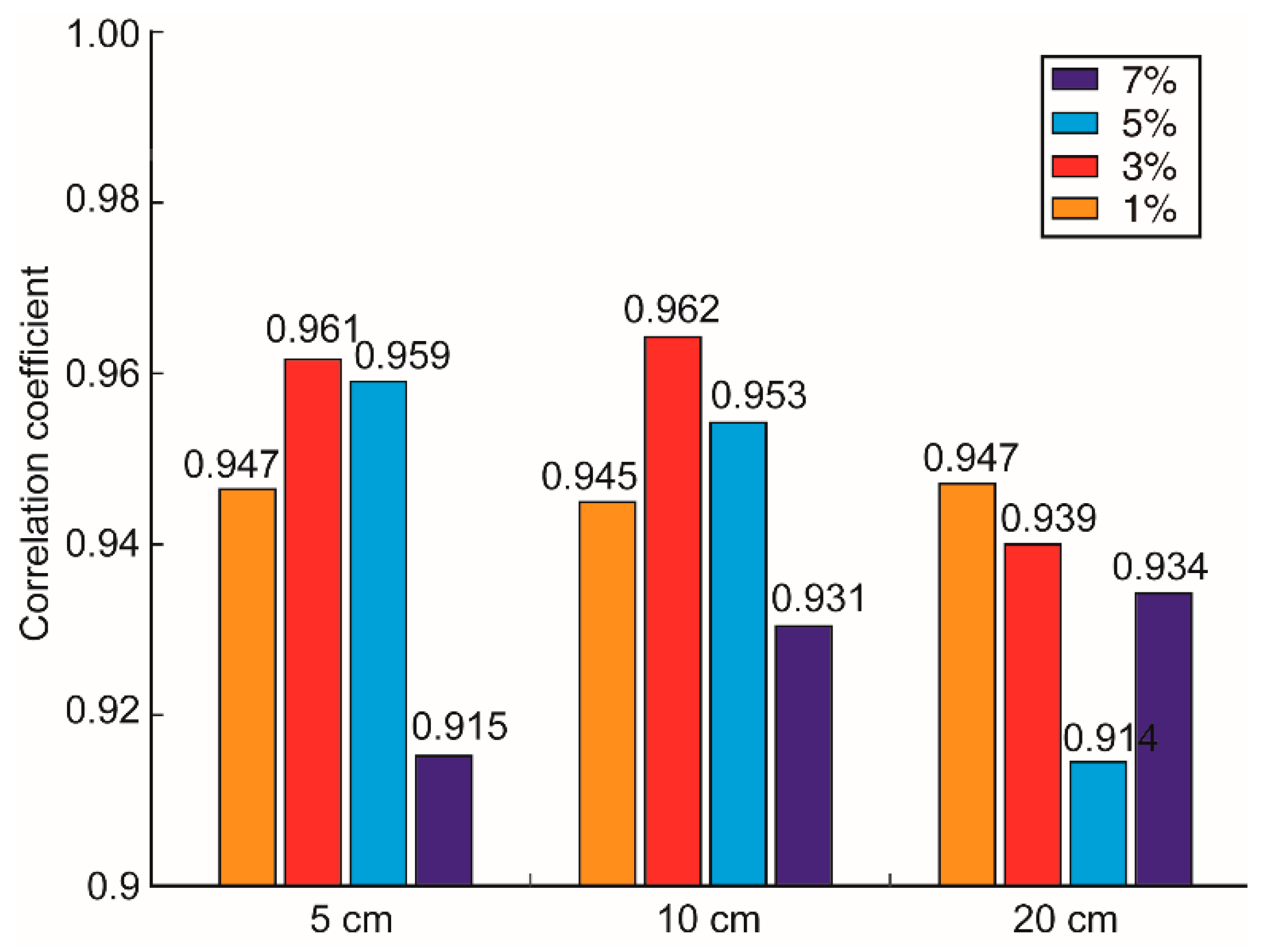
| Correlation Distance (cm) | RMS Perturbation (%) | |||
|---|---|---|---|---|
| 1 | 3 | 5 | 7 | |
| 5 | 0.9469 | 0.9609 | 0.9590 | 0.9147 |
| 10 | 0.9446 | 0.9617 | 0.9527 | 0.9309 |
| 20 | 0.9471 | 0.9394 | 0.9140 | 0.9336 |
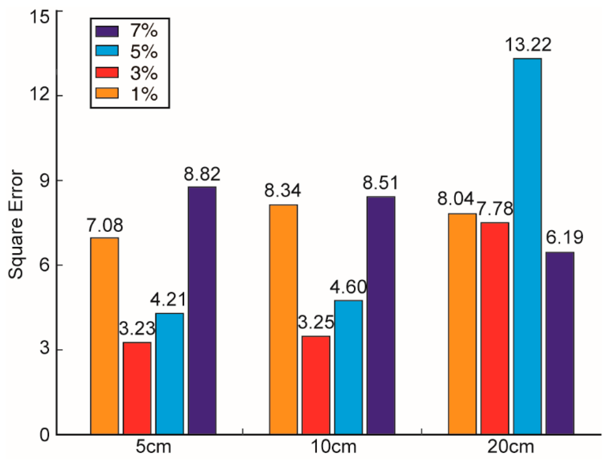
| Correlation Distance (cm) | RMS Perturbation (%) | |||
|---|---|---|---|---|
| 1 | 3 | 5 | 7 | |
| 5 | 7.08 | 3.23 | 4.21 | 8.82 |
| 10 | 8.34 | 3.25 | 4.60 | 8.51 |
| 20 | 8.04 | 7.78 | 13.22 | 6.19 |
Publisher’s Note: MDPI stays neutral with regard to jurisdictional claims in published maps and institutional affiliations. |
© 2021 by the authors. Licensee MDPI, Basel, Switzerland. This article is an open access article distributed under the terms and conditions of the Creative Commons Attribution (CC BY) license (https://creativecommons.org/licenses/by/4.0/).
Share and Cite
Zhang, X.; Lv, W.; Zhang, L.; Zhang, J.; Lin, Y.; Yao, Z. Self-Organization Characteristics of Lunar Regolith Inferred by Yutu-2 Lunar Penetrating Radar. Remote Sens. 2021, 13, 3017. https://doi.org/10.3390/rs13153017
Zhang X, Lv W, Zhang L, Zhang J, Lin Y, Yao Z. Self-Organization Characteristics of Lunar Regolith Inferred by Yutu-2 Lunar Penetrating Radar. Remote Sensing. 2021; 13(15):3017. https://doi.org/10.3390/rs13153017
Chicago/Turabian StyleZhang, Xiang, Wenmin Lv, Lei Zhang, Jinhai Zhang, Yangting Lin, and Zhenxing Yao. 2021. "Self-Organization Characteristics of Lunar Regolith Inferred by Yutu-2 Lunar Penetrating Radar" Remote Sensing 13, no. 15: 3017. https://doi.org/10.3390/rs13153017
APA StyleZhang, X., Lv, W., Zhang, L., Zhang, J., Lin, Y., & Yao, Z. (2021). Self-Organization Characteristics of Lunar Regolith Inferred by Yutu-2 Lunar Penetrating Radar. Remote Sensing, 13(15), 3017. https://doi.org/10.3390/rs13153017