
Neural Network-Based Urban Change Monitoring with Deep-Temporal Multispectral and SAR Remote Sensing Data

 , , , and
Abstract
:
1. Introduction
2. Related Work
3. Data Pre-Processing
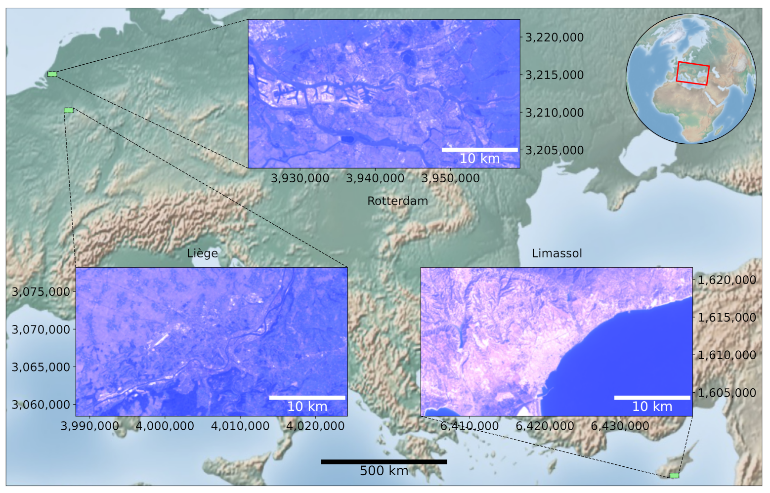
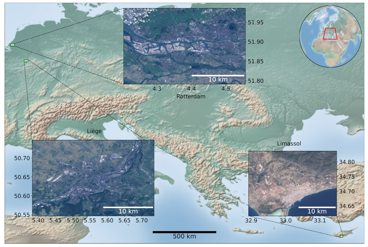
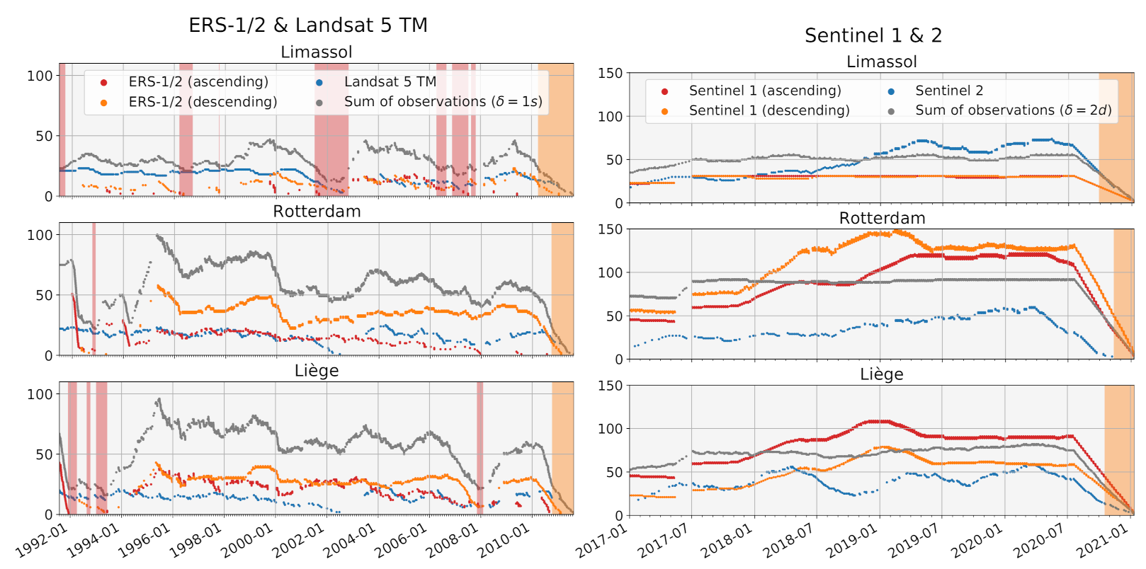
3.1. Selection of AoIs
3.2. Data Acquisition and Pre-Processing
3.2.1. ERS-1/2
3.2.2. Landsat 5 TM
3.2.3. Sentinel 1 and Sentinel 2
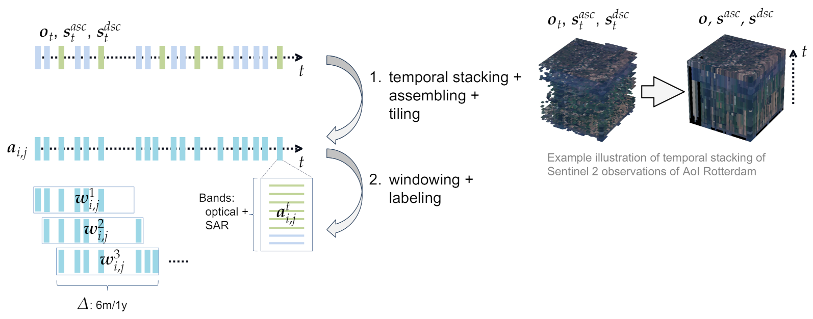
3.3. Time Series Preparation
3.3.1. Temporal Stacking, Assembling, and Tiling
3.3.2. Windowing and Labeling
Saturating the extreme pixel values [...] is unfortunate in our situation where the dominating changes detected are due precisely to those strongly reflecting human-made objects [...]. Pixels that are saturated at several timepoints may not be detected as change pixels, which is potentially wrong. The best way to handle this is to store the data as floats [...].
3.3.3. Expected Noise of Synthetic Labels
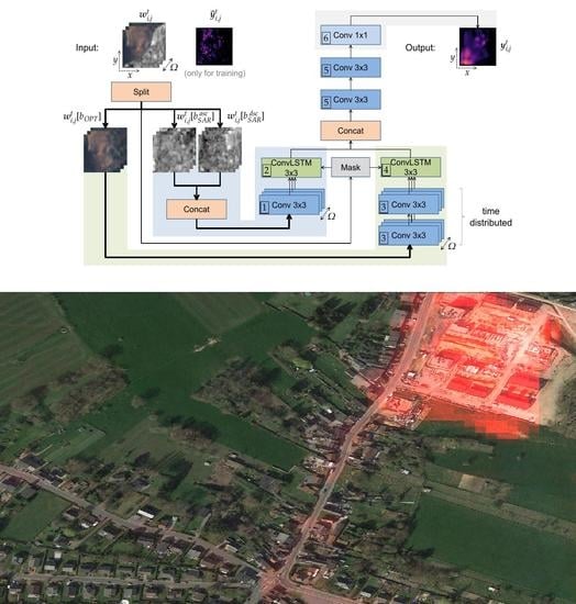
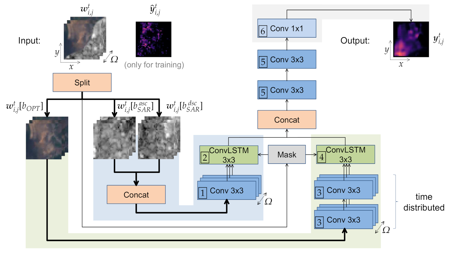
4. Proposed Neural Network
4.1. Architecture
4.2. Training and Validation Methodology
5. Results
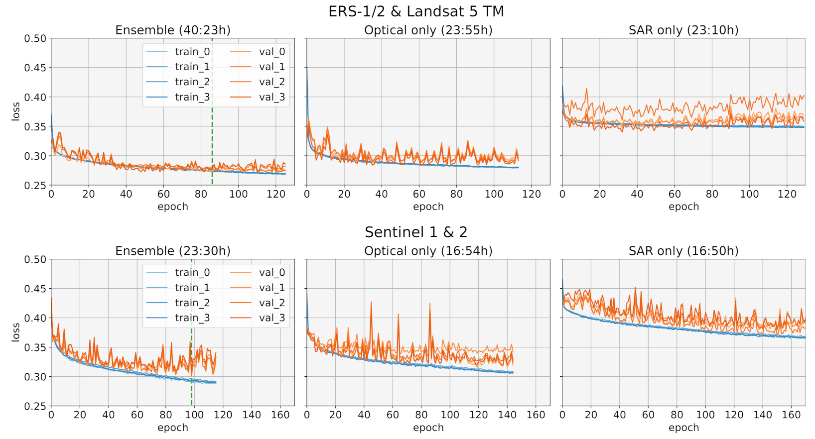
5.1. Training
5.2. Ablation Studies
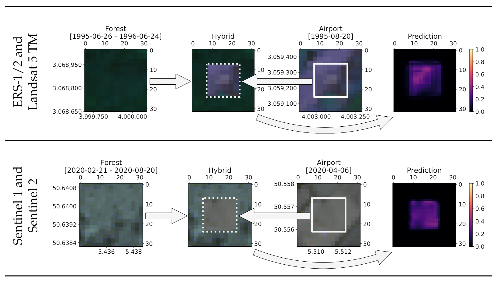
5.2.1. Urban Change Sensitivity
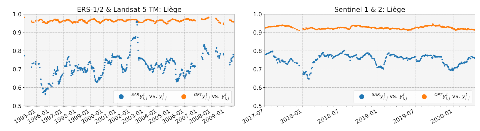
5.2.2. Correlations of SAR and Optical Predictions
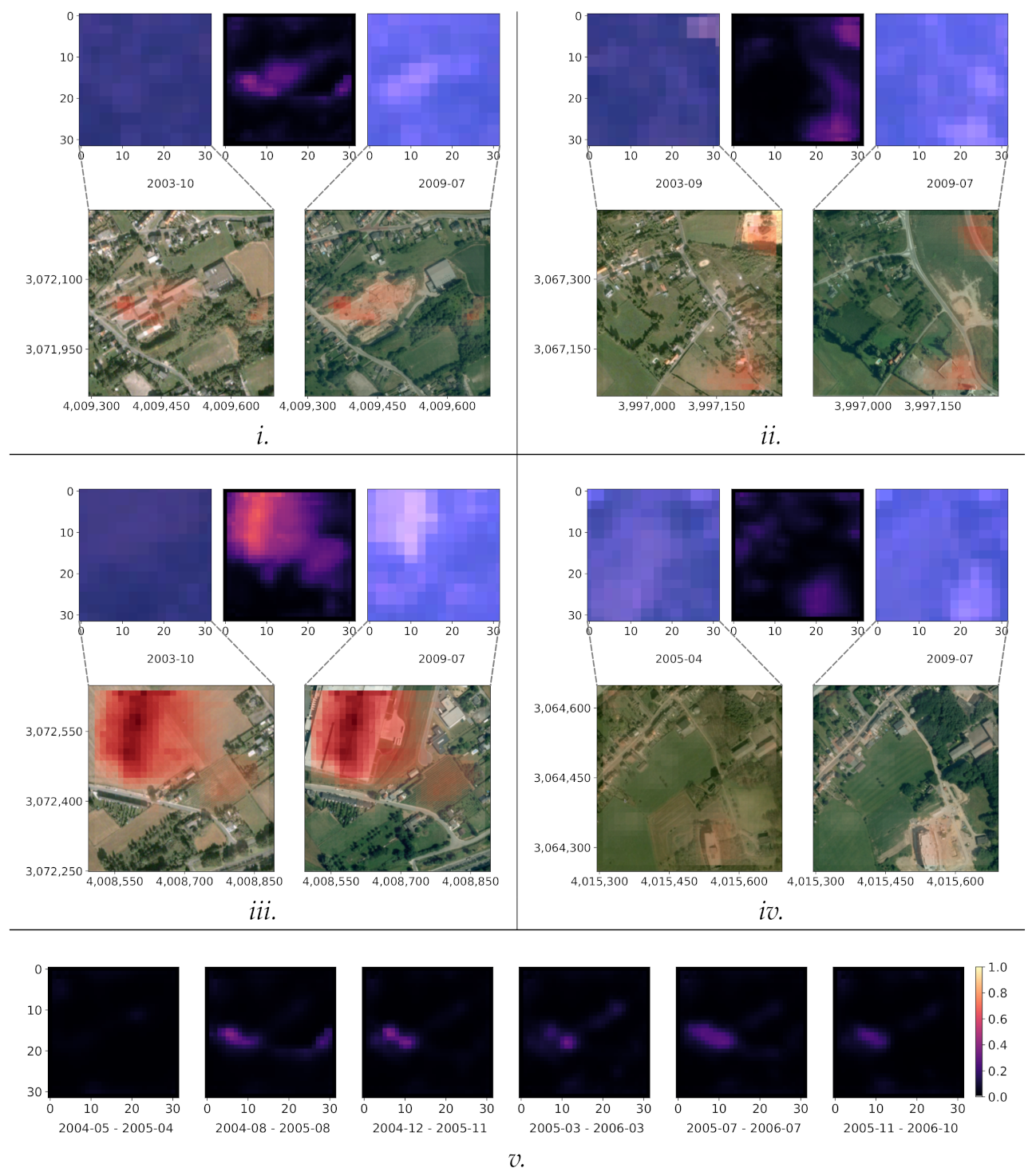
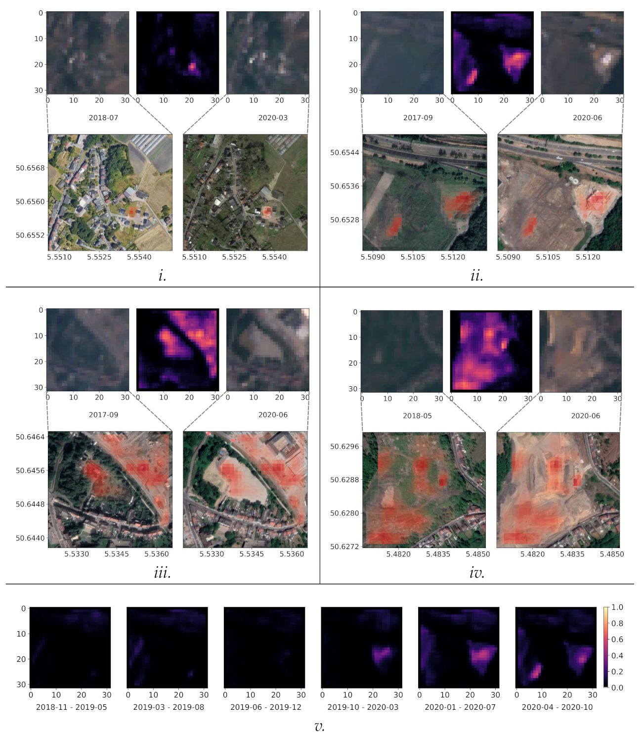
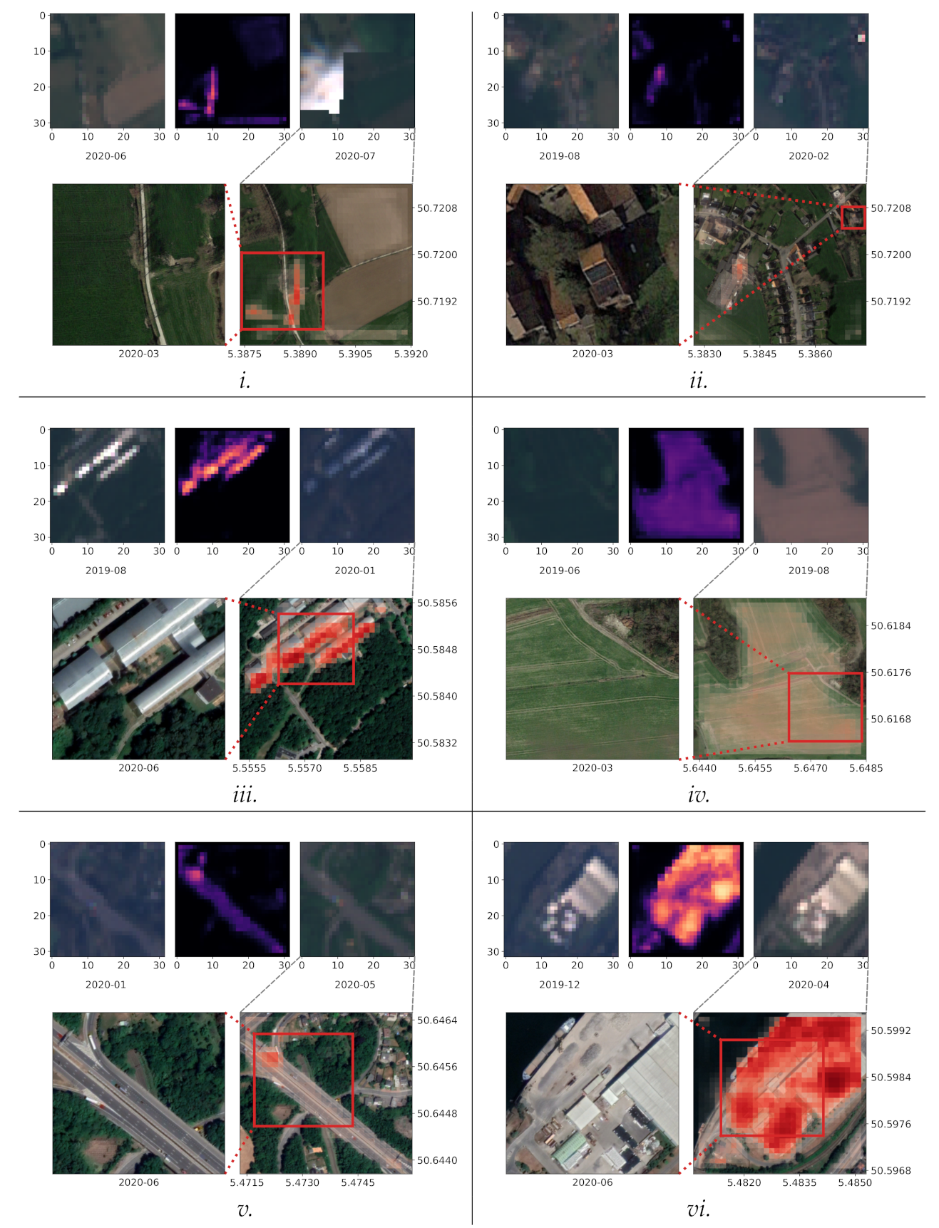
5.3. Qualitative Analysis
6. Discussion
6.1. Current Limitations
6.2. Further Improvements
Images are predicted with a sliding window approach, where the window size equals the patch size used during training. Adjacent predictions overlap by half the size of a patch. The accuracy of segmentation decreases towards the borders of the window. To suppress stitching artifacts and reduce the influence of positions close to the borders, a Gaussian importance weighting is applied, increasing the weight of the center voxels in the softmax aggregation. Test time augmentation by mirroring along all axes is applied.
7. Conclusions
Author Contributions
Funding
Data Availability Statement
Acknowledgments
Conflicts of Interest
Appendix A. Areas of Interest
References
- Singh, A. Review Article Digital change detection techniques using remotely-sensed data. Int. J. Remote Sens. 1989, 10, 989–1003. [Google Scholar] [CrossRef] [Green Version]
- Lehner, A.; Blaschke, T. A Generic Classification Scheme for Urban Structure Types. Remote Sens. 2019, 11, 173. [Google Scholar] [CrossRef] [Green Version]
- You, Y.; Cao, J.; Zhou, W. A Survey of Change Detection Methods Based on Remote Sensing Images for Multi-Source and Multi-Objective Scenarios. Remote Sens. 2020, 12, 2460. [Google Scholar] [CrossRef]
- Patra, S.; Ghosh, S.; Ghosh, A. Semi-supervised Learning with Multilayer Perceptron for Detecting Changes of Remote Sensing Images. In Pattern Recognition and Machine Intelligence; Ghosh, A., De, R.K., Pal, S.K., Eds.; Springer: Berlin/Heidelberg, Germany, 2007; pp. 161–168. [Google Scholar]
- Roy, M.; Routaray, D.; Ghosh, S.; Ghosh, A. Ensemble of Multilayer Perceptrons for Change Detection in Remotely Sensed Images. IEEE Geosci. Remote Sens. Lett. 2014, 11, 49–53. [Google Scholar] [CrossRef]
- Zhu, X.X.; Tuia, D.; Mou, L.; Xia, G.S.; Zhang, L.; Xu, F.; Fraundorfer, F. Deep Learning in Remote Sensing: A Comprehensive Review and List of Resources. IEEE Geosci. Remote Sens. Mag. 2017, 5, 8–36. [Google Scholar] [CrossRef] [Green Version]
- Deng, J.S.; Wang, K.; Deng, Y.H.; Qi, G.J. PCA-based land-use change detection and analysis using multitemporal and multisensor satellite data. Int. J. Remote Sens. 2008, 29, 4823–4838. [Google Scholar] [CrossRef]
- Qin, Y.; Xiao, X.; Dong, J.; Chen, B.; Liu, F.; Zhang, G.; Zhang, Y.; Wang, J.; Wu, X. Quantifying annual changes in built-up area in complex urban-rural landscapes from analyses of PALSAR and Landsat images. ISPRS J. Photogramm. Remote Sens. 2017, 124, 89–105. [Google Scholar] [CrossRef] [Green Version]
- Canty, M.J.; Nielsen, A.A. Automatic radiometric normalization of multitemporal satellite imagery with the iteratively re-weighted MAD transformation. Remote Sens. Environ. 2008, 112, 1025–1036. [Google Scholar] [CrossRef] [Green Version]
- Xiao, P.; Zhang, X.; Wang, D.; Yuan, M.; Feng, X.; Kelly, M. Change detection of built-up land: A framework of combining pixel-based detection and object-based recognition. ISPRS J. Photogramm. Remote Sens. 2016, 119, 402–414. [Google Scholar] [CrossRef]
- Jafari, M.; Majedi, H.; Monavari, S.M.; Alesheikh, A.A.; Zarkesh, M.K. Dynamic simulation of urban expansion through a CA-Markov model Case study: Hyrcanian region, Gilan, Iran. Eur. J. Remote Sens. 2016, 49, 513–529. [Google Scholar] [CrossRef] [Green Version]
- Conradsen, K.; Nielsen, A.A.; Skriver, H. Determining the Points of Change in Time Series of Polarimetric SAR Data. IEEE Trans. Geosci. Remote Sens. 2016, 54, 3007–3024. [Google Scholar] [CrossRef] [Green Version]
- Zhang, M.; Shi, W. A Feature Difference Convolutional Neural Network-Based Change Detection Method. IEEE Trans. Geosci. Remote Sens. 2020, 58, 7232–7246. [Google Scholar] [CrossRef]
- Chen, T.H.K.; Qiu, C.; Schmitt, M.; Zhu, X.X.; Sabel, C.E.; Prishchepov, A.V. Mapping horizontal and vertical urban densification in Denmark with Landsat time-series from 1985 to 2018: A semantic segmentation solution. Remote Sens. Environ. 2020, 251, 112096. [Google Scholar] [CrossRef]
- Yoo, C.; Han, D.; Im, J.; Bechtel, B. Comparison between convolutional neural networks and random forest for local climate zone classification in mega urban areas using Landsat images. ISPRS J. Photogramm. Remote Sens. 2019, 157, 155–170. [Google Scholar] [CrossRef]
- Krizhevsky, A.; Sutskever, I.; Hinton, G.E. ImageNet Classification with Deep Convolutional Neural Networks. In Advances in Neural Information Processing Systems; Pereira, F., Burges, C.J.C., Bottou, L., Weinberger, K.Q., Eds.; Curran Associates, Inc.: Red Hook, NY, USA, 2012; Volume 25. [Google Scholar]
- Deng, C.; Zhu, Z. Continuous subpixel monitoring of urban impervious surface using Landsat time series. Remote Sens. Environ. 2020, 238, 110929. [Google Scholar] [CrossRef]
- Jing, C.; Zhou, W.; Qian, Y.; Yu, W.; Zheng, Z. A novel approach for quantifying high-frequency urban land cover changes at the block level with scarce clear-sky Landsat observations. Remote Sens. Environ. 2021, 255, 112293. [Google Scholar] [CrossRef]
- Pandey, D.; Tiwari, K. Extraction of urban built-up surfaces and its subclasses using existing built-up indices with separability analysis of spectrally mixed classes in AVIRIS-NG imagery. Adv. Space Res. 2020, 66, 1829–1845. [Google Scholar] [CrossRef]
- Estoque, R.C.; Murayama, Y. Classification and change detection of built-up lands from Landsat-7 ETM+ and Landsat-8 OLI/TIRS imageries: A comparative assessment of various spectral indices. Ecol. Indic. 2015, 56, 205–217. [Google Scholar] [CrossRef]
- Chen, J.; Chen, S.; Yang, C.; He, L.; Hou, M.; Shi, T. A comparative study of impervious surface extraction using Sentinel-2 imagery. Eur. J. Remote Sens. 2020, 53, 274–292. [Google Scholar] [CrossRef]
- Guha, S.; Govil, H.; Gill, N.; Dey, A. A long-term seasonal analysis on the relationship between LST and NDBI using Landsat data. Quat. Int. 2021, 575–576, 249–258. [Google Scholar] [CrossRef]
- Xu, H. Analysis of Impervious Surface and its Impact on Urban Heat Environment using the Normalized Difference Impervious Surface Index (NDISI). Photogramm. Eng. Remote Sens. 2010, 76, 557–565. [Google Scholar] [CrossRef]
- Mitra, D.; Banerji, S. Urbanisation and changing waterscapes: A case study of New Town, Kolkata, West Bengal, India. Appl. Geogr. 2018, 97, 109–118. [Google Scholar] [CrossRef]
- Zhang, S.; Yang, K.; Li, M.; Ma, Y.; Sun, M. Combinational Biophysical Composition Index (CBCI) for Effective Mapping Biophysical Composition in Urban Areas. IEEE Access 2018, 6, 41224–41237. [Google Scholar] [CrossRef]
- Zhong, J.; Li, Z.; Sun, Z.; Tian, Y.; Yang, F. The spatial equilibrium analysis of urban green space and human activity in Chengdu, China. J. Clean. Prod. 2020, 259, 120754. [Google Scholar] [CrossRef]
- Gomez-Chova, L.; Fernández-Prieto, D.; Calpe, J.; Soria, E.; Vila, J.; Camps-Valls, G. Urban monitoring using multi-temporal SAR and multi-spectral data. Pattern Recognit. Lett. 2006, 27, 234–243. [Google Scholar] [CrossRef]
- Sinha, S.; Santra, A.; Mitra, S.S. Semi-automated impervious feature extraction using built-up indices developed from space-borne optical and SAR remotely sensed sensors. Adv. Space Res. 2020, 66, 1372–1385. [Google Scholar] [CrossRef]
- Moreira, A.; Prats-Iraola, P.; Younis, M.; Krieger, G.; Hajnsek, I.; Papathanassiou, K.P. A tutorial on synthetic aperture radar. IEEE Geosci. Remote Sens. Mag. 2013, 1, 6–43. [Google Scholar] [CrossRef] [Green Version]
- Zhang, H.; Lin, H.; Li, Y.; Zhang, Y.; Fang, C. Mapping urban impervious surface with dual-polarimetric SAR data: An improved method. Landsc. Urban Plan. 2016, 151, 55–63. [Google Scholar] [CrossRef]
- Benedetti, A.; Picchiani, M.; Del Frate, F. Sentinel-1 and Sentinel-2 Data Fusion for Urban Change Detection. In Proceedings of the IGARSS 2018-2018 IEEE International Geoscience and Remote Sensing Symposium, Valencia, Spain, 22–27 July 2018; pp. 1962–1965. [Google Scholar] [CrossRef]
- Muro, J.; Canty, M.; Conradsen, K.; Hüttich, C.; Nielsen, A.A.; Skriver, H.; Remy, F.; Strauch, A.; Thonfeld, F.; Menz, G. Short-Term Change Detection in Wetlands Using Sentinel-1 Time Series. Remote Sens. 2016, 8, 795. [Google Scholar] [CrossRef] [Green Version]
- Ansari, R.A.; Buddhiraju, K.M.; Malhotra, R. Urban change detection analysis utilizing multiresolution texture features from polarimetric SAR images. Remote Sens. Appl. Soc. Environ. 2020, 20, 100418. [Google Scholar] [CrossRef]
- Manzoni, M.; Monti-Guarnieri, A.; Molinari, M.E. Joint exploitation of spaceborne SAR images and GIS techniques for urban coherent change detection. Remote Sens. Environ. 2021, 253, 112152. [Google Scholar] [CrossRef]
- Susaki, J.; Kajimoto, M.; Kishimoto, M. Urban density mapping of global megacities from polarimetric SAR images. Remote Sens. Environ. 2014, 155, 334–348. [Google Scholar] [CrossRef] [Green Version]
- Jiang, M.; Hooper, A.; Tian, X.; Xu, J.; Chen, S.N.; Ma, Z.F.; Cheng, X. Delineation of built-up land change from SAR stack by analysing the coefficient of variation. ISPRS J. Photogramm. Remote Sens. 2020, 169, 93–108. [Google Scholar] [CrossRef]
- Caye Daudt, R.; Le Saux, B.; Boulch, A.; Gousseau, Y. Urban Change Detection for Multispectral Earth Observation Using Convolutional Neural Networks. In Proceedings of the IEEE International Geoscience and Remote Sensing Symposium (IGARSS), Valencia, Spain, 22–27 July 2018. [Google Scholar]
- Caye Daudt, R.; Le Saux, B.; Boulch, A. Fully Convolutional Siamese Networks for Change Detection. In Proceedings of the 2018 25th IEEE International Conference on Image Processing (ICIP), Athens, Greece, 7–10 October 2018; pp. 4063–4067. [Google Scholar] [CrossRef] [Green Version]
- Benedek, C.; Sziranyi, T. Change Detection in Optical Aerial Images by a Multilayer Conditional Mixed Markov Model. IEEE Trans. Geosci. Remote Sens. 2009, 47, 3416–3430. [Google Scholar] [CrossRef] [Green Version]
- Kundu, K.; Halder, P.; Mandal, J.K. Urban Change Detection Analysis during 1978–2017 at Kolkata, India, using Multi-temporal Satellite Data. J. Indian Soc. Remote Sens. 2020, 48, 1535–1554. [Google Scholar] [CrossRef]
- Lu, D.; Moran, E.; Hetrick, S. Detection of impervious surface change with multitemporal Landsat images in an urban–rural frontier. ISPRS J. Photogramm. Remote Sens. 2011, 66, 298–306. [Google Scholar] [CrossRef] [PubMed] [Green Version]
- Ban, Y.; Yousif, O.A. Multitemporal Spaceborne SAR Data for Urban Change Detection in China. IEEE J. Sel. Top. Appl. Earth Obs. Remote Sens. 2012, 5, 1087–1094. [Google Scholar] [CrossRef]
- Wania, A.; Kemper, T.; Tiede, D.; Zeil, P. Mapping recent built-up area changes in the city of Harare with high resolution satellite imagery. Appl. Geogr. 2014, 46, 35–44. [Google Scholar] [CrossRef]
- Demir, I.; Koperski, K.; Lindenbaum, D.; Pang, G.; Huang, J.; Basu, S.; Hughes, F.; Tuia, D.; Raskar, R. DeepGlobe 2018: A Challenge to Parse the Earth through Satellite Images. In Proceedings of the 2018 IEEE/CVF Conference on Computer Vision and Pattern Recognition Workshops (CVPRW), Salt Lake City, UT, USA, 18–22 June 2018; pp. 172–181. [Google Scholar] [CrossRef] [Green Version]
- Esch, T.; Asamer, H.; Bachofer, F.; Balhar, J.; Boettcher, M.; Boissier, E.; d’ Angelo, P.; Gevaert, C.M.; Hirner, A.; Jupova, K.; et al. Digital world meets urban planet–new prospects for evidence-based urban studies arising from joint exploitation of big earth data, information technology and shared knowledge. Int. J. Digit. Earth 2020, 13, 136–157. [Google Scholar] [CrossRef]
- Marconcini, M.; Metz-Marconcini, A.; Üreyen, S.; Palacios-Lopez, D.; Hanke, W.; Bachofer, F.; Zeidler, J.; Esch, T.; Gorelick, N.; Kakarla, A.; et al. Outlining where humans live, the World Settlement Footprint 2015. Sci. Data 2020, 7, 242. [Google Scholar] [CrossRef] [PubMed]
- Esch, T.; Heldens, W.; Hirner, A.; Keil, M.; Marconcini, M.; Roth, A.; Zeidler, J.; Dech, S.; Strano, E. Breaking new ground in mapping human settlements from space–The Global Urban Footprint. ISPRS J. Photogramm. Remote Sens. 2017, 134, 30–42. [Google Scholar] [CrossRef] [Green Version]
- King, M.D.; Platnick, S.; Menzel, W.P.; Ackerman, S.A.; Hubanks, P.A. Spatial and Temporal Distribution of Clouds Observed by MODIS Onboard the Terra and Aqua Satellites. IEEE Trans. Geosci. Remote Sens. 2013, 51, 3826–3852. [Google Scholar] [CrossRef]
- Nielsen, A.A.; Canty, M.J.; Skriver, H.; Conradsen, K. Change detection in multi-temporal dual polarization Sentinel-1 data. In Proceedings of the 2017 IEEE International Geoscience and Remote Sensing Symposium (IGARSS), Fort Worth, TX, USA, 23–28 July 2017; pp. 3901–3904. [Google Scholar] [CrossRef]
- Chen, J.; Yang, K.; Chen, S.; Yang, C.; Zhang, S.; He, L. Enhanced normalized difference index for impervious surface area estimation at the plateau basin scale. J. Appl. Remote Sens. 2019, 13, 016502. [Google Scholar] [CrossRef] [Green Version]
- Xu, H. Modification of normalised difference water index (NDWI) to enhance open water features in remotely sensed imagery. Int. J. Remote Sens. 2006, 27, 3025–3033. [Google Scholar] [CrossRef]
- Faridatul, M.I.; Wu, B. Automatic Classification of Major Urban Land Covers Based on Novel Spectral Indices. ISPRS Int. J. Geo-Inf. 2018, 7, 453. [Google Scholar] [CrossRef] [Green Version]
- Diakogiannis, F.; Waldner, F.; Caccetta, P.; Wu, C. ResUNet-a: A deep learning framework for semantic segmentation of remotely sensed data. ISPRS J. Photogramm. Remote Sens. 2020, 162, 94–114. [Google Scholar] [CrossRef] [Green Version]
- Shahroudnejad, A. A Survey on Understanding, Visualizations, and Explanation of Deep Neural Networks. arXiv 2021, arXiv:2102.01792. [Google Scholar]
- LeCun, Y.; Boser, B.; Denker, J.S.; Henderson, D.; Howard, R.E.; Hubbard, W.; Jackel, L.D. Backpropagation Applied to Handwritten Zip Code Recognition. Neural Comput. 1989, 1, 541–551. [Google Scholar] [CrossRef]
- Shi, X.; Chen, Z.; Wang, H.; Yeung, D.Y.; Wong, W.k.; Woo, W.c. Convolutional LSTM Network: A Machine Learning Approach for Precipitation Nowcasting. In Proceedings of the 28th International Conference on Neural Information Processing Systems-Volume 1, Montreal, QC, Canada, 7–12 December 2015; MIT Press: Cambridge, MA, USA, 2015; pp. 802–810. [Google Scholar]
- Hochreiter, S.; Schmidhuber, J. Long Short-Term Memory. Neural Comput. 1997, 9, 1735–1780. [Google Scholar] [CrossRef] [PubMed]
- Nguyen, L.D.; Gao, R.; Lin, D.; Lin, Z. Biomedical image classification based on a feature concatenation and ensemble of deep CNNs. J. Ambient. Intell. Humaniz. Comput. 2019, 1–13. [Google Scholar] [CrossRef]
- Ju, C.; Bibaut, A.; van der Laan, M. The relative performance of ensemble methods with deep convolutional neural networks for image classification. J. Appl. Stat. 2018, 45, 2800–2818. [Google Scholar] [CrossRef]
- Glorot, X.; Bordes, A.; Bengio, Y. Deep Sparse Rectifier Neural Networks. In Proceedings of the Fourteenth International Conference on Artificial Intelligence and Statistics, Fort Lauderdale, FL, USA, 11–13 April 2011; Gordon, G., Dunson, D., Dudík, M., Eds.; PMLR: Cambridge, MA, USA, 2011; Volume 15, pp. 315–323. [Google Scholar]
- Gal, Y.; Ghahramani, Z. A Theoretically Grounded Application of Dropout in Recurrent Neural Networks. In Proceedings of the 30th International Conference on Neural Information Processing Systems, Barcelona, Spain, 5 December 2016; Curran Associates Inc.: Red Hook, NY, USA, 2016; pp. 1027–1035. [Google Scholar]
- Ma, J.; Chen, J.; Ng, M.; Huang, R.; Li, Y.; Li, C.; Yang, X.; Martel, A.L. Loss Odyssey in Medical Image Segmentation. Med Image Anal. 2021, 71, 102035. [Google Scholar] [CrossRef] [PubMed]
- Reina, G.A.; Panchumarthy, R.; Thakur, S.P.; Bastidas, A.; Bakas, S. Systematic Evaluation of Image Tiling Adverse Effects on Deep Learning Semantic Segmentation. Front. Neurosci. 2020, 14, 65. [Google Scholar] [CrossRef]
- Huang, B.; Reichman, D.; Collins, L.M.; Bradbury, K.; Malof, J.M. Dense labeling of large remote sensing imagery with convolutional neural networks: A simple and faster alternative to stitching output label maps. arXiv 2018, arXiv:1805.12219. [Google Scholar]
- Huang, B.; Reichman, D.; Collins, L.M.; Bradbury, K.; Malof, J.M. Tiling and Stitching Segmentation Output for Remote Sensing: Basic Challenges and Recommendations. arXiv 2019, arXiv:1805.12219. [Google Scholar]
- Isensee, F.; Jaeger, P.F.; Kohl, S.A.A.; Petersen, J.; Maier-Hein, K.H. nnU-Net: A self-configuring method for deep learning-based biomedical image segmentation. Nat. Methods 2021, 18, 203–211. [Google Scholar] [CrossRef]
- Sergeev, A.; Balso, M.D. Horovod: Fast and easy distributed deep learning in TensorFlow. arXiv 2018, arXiv:1802.05799. [Google Scholar]
- Zinkevich, M.; Weimer, M.; Li, L.; Smola, A. Parallelized Stochastic Gradient Descent. In Advances in Neural Information Processing Systems; Lafferty, J., Williams, C., Shawe-Taylor, J., Zemel, R., Culotta, A., Eds.; Curran Associates, Inc.: Red Hook, NY, USA, 2010; Volume 23. [Google Scholar]
- Chen, J.; Monga, R.; Bengio, S.; Jozefowicz, R. Revisiting Distributed Synchronous SGD. In Proceedings of the Workshop Track of the International Conference on Learning Representations, ICLR, San Juan, Puerto Rico, 2–4 May 2016. [Google Scholar]
- Roth, H.R.; Oda, H.; Zhou, X.; Shimizu, N.; Yang, Y.; Hayashi, Y.; Oda, M.; Fujiwara, M.; Misawa, K.; Mori, K. An application of cascaded 3D fully convolutional networks for medical image segmentation. Comput. Med Imaging Graph. 2018, 66, 90–99. [Google Scholar] [CrossRef] [PubMed] [Green Version]
- Kendall, M.G. A new measure of rank correlation. Biometrika 1938, 30, 81–93. [Google Scholar] [CrossRef]
- Fisher, P. The pixel: A snare and a delusion. Int. J. Remote Sens. 1997, 18, 679–685. [Google Scholar] [CrossRef]
- Song, H.; Kim, M.; Park, D.; Lee, J. Learning from Noisy Labels with Deep Neural Networks: A Survey. arXiv 2020, arXiv:2007.08199. [Google Scholar]
- Nguyen, T.; Mummadi, C.K.; Ngo, T.P.N.; Nguyen, T.H.P.; Beggel, L.; Brox, T. SELF: Learning to filter noisy labels with self-ensembling. In Proceedings of the International Conference on Learning Representations (ICLR), Addis Ababa, Ethiopia, 26–30 April 2020. [Google Scholar]
- Valentin, B.; Gale, L.; Boulahya, H.; Charalampopoulou, B.; Christos, K.C.; Poursanidis, D.; Chrysoulakis, N.; Svatoň, V.; Zitzlsberger, G.; Podhoranyi, M.; et al. Blended-using blockchain and deep learning for space data processing. In Proceedings of the 2021 Conference on Big Data from Space, Virtual Event, 18–20 May 2021; Soille, P., Loekken, S., Albani, S., Eds.; Publications Office of the European Union: Luxembourg, 2021; pp. 97–100. [Google Scholar] [CrossRef]


| Change Detection Method | Missions | Number of Observations | Resolution (m/pixel) | Area () | Authors/Reference |
|---|---|---|---|---|---|
| Fully Convolutional Siamese | OSCD [37] (Sentinel 2), | 24 pairs (2015–2018), | down to 10, | 864.0 (OSCD) | Daudt et al. [38] |
| Networks (FCNN) | AC [39] (Aerial, RGB only) | 12 pairs (2000–2007) | 1.5 | 16.3 (AC) | |
| Multiple- Coherent Change | Sentinel 1 | 17 (2015–2016) | 10 | 120.0 | Manzoni et al. [34] |
| Detection (M-CCD) | |||||
| Pulse Coupled Neural Network | Sentinel 1 and 2 | 6 pairs (2015–2017) | 10 | 1.75 | Benedetti et al. [31] |
| Curvelet, Contourlet, and | UAVSAR | 2 pairs (2009 and 2015) | 3.2 | N/A (small) | Ansari et al. [33] |
| Wavelet Transforms | |||||
| Maximum Likelihood | Landsat 2, 5, 7, and 8 | 5 (1978–2017) | 30, 60 for Landsat 2 | 1129.4 | Kundu et al. [40] |
| TSFLC: Temporal Segmentation and | Landsat TM/ETM+, OLI | 68 (1986–2017) | N/A (ca. 30) | 1997 | Jing et al. [18] |
| Trajectory Classification | |||||
| Omnibus and Change Vector | Sentinel 1 and | 12+11 (2014–2016) | both 30 | 490 and 3500 | Muro et al. [32] |
| Analysis (CVA) | Landsat 7,8 | 8+6 (2015) | |||
| Decision Trees | ALOS PALSAR and | 174 (eff. 55) and | 30 | 17,076 | Qin et al. [8] |
| Landsat TM/ETM+ | 20 (2006–2011) | ||||
| Regression Model | Landsat MSS/TM/ETM+ and | 10 (1977–2008) and | 30 and | 3660 | Lu et al. [41] |
| QuickBird | 2 (calibration only) | 0.6 | |||
| Modified Ratio Operator + | ENVISAT ASAR and | 2 pairs (1998/99–2008) | 30 | N/A (small) | Ban et al. [42] |
| Kittler-Illingworth | ERS-2 | ||||
| Topologically Enabled | Spot 2 and 5 | 3 (2004–2010) | 10 and 5/2.5 | 940 | Wania et al. [43] |
| Hierarchical Framework | |||||
| Spectral and Textural | IKONOS, GF-1, and | total of 6 (1, 2, and 3) | 0.5–2 | 1.4, 0.4–0.45, and | Xiao et al. [10] |
| Differences | Aerial | pairs for 2000–2016 | 0.24–1.1 | ||
| ERCNN-DRS | ERS-1/2 and Landsat 5 TM, | 1121 and 638 (1991–2011), | 30, | see Table 2 | our study |
| Sentinel 1 and 2 | 2067 and 640 (2017–2021) | 10 |
| Site | AoI Bounding Box | Reference | Area | |
|---|---|---|---|---|
| (Long, Lat)/(East, North) | System | (km2) | ||
| ERS-1/2 and Landsat 5 TM | Rotterdam | (3,923,101, 3,202,549), (3,959,241, 3,222,337) | EPSG:3035 | 712.9 |
| Liège | (3,988,121, 3,058,430), (4,024,261, 3,078,219) | EPSG:3035 | 713.3 | |
| Limassol | (6,403,482, 1,601,833), (6,439,623, 1,621,621) | EPSG:3035 | 718.6 | |
| Resolution | SAR: 12.5 m/pixel | |||
| Optical: 30 m/pixel (interpolated to 12.5 m/pixel) | ||||
| Sentinel 1 and Sentinel 2 | Rotterdam | (4.2033, 51.7913), (4.5566, 51.9854) | EPSG:4326 | 523.6 |
| Liège | (5.3827, 50.5474), (5.7280, 50.7350) | EPSG:4326 | 508.4 | |
| Limassol | (32.8925, 34.6159), (33.1482, 34.8365) | EPSG:4326 | 576.2 | |
| Resolution | SAR/Optical: 10 m/pixel | |||
| Site | SAR Observations (Ascending and Descending) | Optical Multispectral Observations | |
|---|---|---|---|
| ERS-1/2 and Landsat 5 TM | Rotterdam | 974 (−118) | 753 (−434) |
| Liège | 934 (−89) | 888 (−620) | |
| Limassol | 291 (−27) | 380 (−61) | |
| Source/Product | ESA/SAR_IMP_1P | USGS/L4-5 TM C1 L1 | |
| Sentinel 1 and Sentinel 2 | Rotterdam | 1603 (−4) | 278 (−10) |
| Liège | 1040 (−0) | 332 (−35) | |
| Limassol | 468 (−0) | 407 (−35) | |
| Source/Product | Sentinel Hub/ | Sentinel Hub/L1C | |
| SENTINEL1_IW_[ASC|DSC] |
| Parameter | Mnemonic | ERS-1/2 and Landsat 5 TM | Sentinel 1 and 2 | ||
|---|---|---|---|---|---|
| Rotterdam and Liège | Limassol | Rotterdam and Liège | Limassol | ||
| SAR bands | 1 (VV) | 1 (VV) | 2 (VV + VH) | 2 (VV + VH) | |
| optical bands | 7 | 7 | 13 | 13 | |
| shift | 0.25 | 0.5 | 0.25 | 0.5 | |
| scale | 30.0 | 30.0 | 10.0 | 10.0 | |
| significance | 0.1 | 0.1 | 0.001 | 0.001 | |
| ENL | 3 | 3 | 4 | 4 | |
| step | |||||
| min. window size | 25 | 25 | 35 | 35 | |
| max. window size | 110 | 110 | 92 | 92 | |
| Symbol | Landsat 5 TM | Sentinel 2 | ||||
|---|---|---|---|---|---|---|
| Band | Spectral | Resolution | Band | Spectral | Resolution | |
| Range (nm) | (m/pixel) | Range (nm) | (m/pixel) | |||
| TM1 | 450–520 | 30 | B2 | 459–525 | 10 | |
| TM2 | 520–600 | 30 | B3 | 541–578 | 10 | |
| TM3 | 630–690 | 30 | B4 | 649–680 | 10 | |
| TM4 | 760–900 | 30 | B8 | 780–886 | 10 | |
| TM5 | 1550–1750 | 30 | B11 | 1565–1659 | 20 | |
| TM7 | 2080–2350 | 30 | B12 | 2098–2290 | 20 | |
| Hyper- Parameters | Configurations | ||||||
|---|---|---|---|---|---|---|---|
| ERS-1/2 and Landsat 5 TM | Filters | 4 | 4 | 20 | 20 | 8 | 1 |
| Kernel | |||||||
| Stride | |||||||
| Activation(s) | ReLU | tanh, hard | ReLU | tanh, hard | ReLU | sigmoid | |
| sigmoid | sigmoid | ||||||
| Dropout | 0.4 | 0.4 | |||||
| Sentinel 1 and Sentinel 2 | Filters | 10 | 10 | 26 | 26 | 8 | 1 |
| Kernel | |||||||
| Stride | |||||||
| Activation(s) | ReLU | tanh, hard | ReLU | tanh, hard | ReLU | sigmoid | |
| sigmoid | sigmoid | ||||||
| Dropout | 0.4 | 0.4 | |||||
Publisher’s Note: MDPI stays neutral with regard to jurisdictional claims in published maps and institutional affiliations. |
© 2021 by the authors. Licensee MDPI, Basel, Switzerland. This article is an open access article distributed under the terms and conditions of the Creative Commons Attribution (CC BY) license (https://creativecommons.org/licenses/by/4.0/).
Share and Cite
Zitzlsberger, G.; Podhorányi, M.; Svatoň, V.; Lazecký, M.; Martinovič, J. Neural Network-Based Urban Change Monitoring with Deep-Temporal Multispectral and SAR Remote Sensing Data. Remote Sens. 2021, 13, 3000. https://doi.org/10.3390/rs13153000
Zitzlsberger G, Podhorányi M, Svatoň V, Lazecký M, Martinovič J. Neural Network-Based Urban Change Monitoring with Deep-Temporal Multispectral and SAR Remote Sensing Data. Remote Sensing. 2021; 13(15):3000. https://doi.org/10.3390/rs13153000
Chicago/Turabian StyleZitzlsberger, Georg, Michal Podhorányi, Václav Svatoň, Milan Lazecký, and Jan Martinovič. 2021. "Neural Network-Based Urban Change Monitoring with Deep-Temporal Multispectral and SAR Remote Sensing Data" Remote Sensing 13, no. 15: 3000. https://doi.org/10.3390/rs13153000
APA StyleZitzlsberger, G., Podhorányi, M., Svatoň, V., Lazecký, M., & Martinovič, J. (2021). Neural Network-Based Urban Change Monitoring with Deep-Temporal Multispectral and SAR Remote Sensing Data. Remote Sensing, 13(15), 3000. https://doi.org/10.3390/rs13153000