Abstract
Hyperspectral remote sensing can obtain both spatial and spectral information of ground objects. It is an important prerequisite for a hyperspectral remote sensing application to make good use of spectral and image features. Therefore, we improved the Convolutional Neural Network (CNN) model by extracting interior-edge-adjacency features of building roof and proposed a new CNN model with a flexible structure: Building Roof Identification CNN (BRI-CNN). Our experimental results demonstrated that the BRI-CNN can not only extract interior-edge-adjacency features of building roof, but also change the weight of these different features during the training process, according to selected samples. Our approach was tested using the Indian Pines (IP) data set and our comparative study indicates that the BRI-CNN model achieves at least 0.2% higher overall accuracy than that of the capsule network model, and more than 2% than that of CNN models.
1. Introduction
Compared to traditional remote sensing, hyperspectral remote sensing can not only obtain spatial information, but also acquire digital spectral images of materials on the earth surface using many narrow contiguous spectral bands. With massive spectrums of information, it shows a strong superiority in object detection and material identification [1]. Additionally, until now hyperspectral images (HSI) have been used in several applications, ranging from agriculture and forestry to global environmental change research [2,3,4,5]. However, due to the high dimensionality of hyperspectral data, problems regarding overfitting can always occur. To avoid this problem, methods such as Principal Component Analysis (PCA), Linear Discriminant Analysis (LDA), and Independent Component Analysis (ICA) [6,7,8] were applied. After that, traditional machine learning algorithms, such as Support Vector Machine (SVM) [9] and Neural Network (NN) [10] have been used for classification. Not coincidentally, it is difficult to perform recognition and classification tasks using these conventional machine learning algorithms because of high redundancy and nonlinear of HSI [11,12,13,14,15,16,17]. But deep learning technology solves these problems to some extent.
Deep learning (DL), a part of a broader family of machine learning methods, is widely used in computer vision, and information retrieval. In recent years, Convolutional Neural Network (CNN) models [18], Dense Networks [19], Capsule Networks [20], and the Deep Belief Network (DBN) are proposed to the imagery identification tasks in remote sensing. Cao et al. [21,22,23,24,25,26,27,28] studied the application of CNN or DBN to the hyperspectral remote sensing domain. Zhong et al. [29] introduced an end-to-end spectral-spatial residual network (SSRN). For HSI classification, a special state-of-the-art CNN model, ResNet, was used [30]. Gao, Lim, and Jia [31] used a CNN model with multiple features. Li, Xie, and Li [32] introduced a CNN model with a new spatial feature-based strategy for band selection. Chen et al. [33] introduced a conventional CNN model. Paoletti et al. [34] proposed a CNN model based on capsule network, a new model that is broadly used in computer vision field nowadays. CNN combines the spatial and spectral features via multichannel convolutional kernels that can integrate the information in the spatial and spectral dimensions into one and the same feature map. In convolution, because spatial and spectral information are mixed and become inseparable, the proportion of the two different features is stationary and unalterable. In other words, in these models, the weight of the two features in different areas with the same type of land-cover cannot be adjusted.
To strengthen spectral and spatial features, we propose a Building Roof Identification Convolutional Neural Network (BRI-CNN) based on interior-edge-adjacency features, which has a more flexible structure. We applied three different scales of convolutional kernels directly to the input image, including a set of 1 × 1 kernels aimed at the interior features of building roof (also named as spectral features), a set of 3 × 3 kernels to extract edge features, and a set of 5 × 5 kernels for adjacency features. To classify a pixel, we acquired its 9 × 9 neighbours. If the pixel is located near the boundary of different types of land-cover, the spatial features of the input image are more useful. When the central pixel is located in the interior of one with the same type of land-cover, the spatial features lose their effectiveness, and the spectral features are dominant. BRI-CNN was designed and tuned using our own HSI data. To evaluate BRI-CNN more objectively, some public data sets were also used.
The rest of the paper is organized as follows. Section 2 briefly introduced the data and methods we used and provided the hyper-parameters of our model. Section 3 presented the experimental results during the determination of hyper-parameters and compared the performance of BRI-CNN and other models. This is followed in Section 4 by a conclusion of our research.
2. Data and Methods
2.1. Data
A hyperspectral image, containing 64 bands in the range of 0.462 to 10.25 µm, was obtained in Beijing in 2001, using a push-broom hyperspectral imager (PHI) sensor. With a spatial resolution of 1 m, we labelled some pixels to represent different kinds of rooftop materials as samples on GIS software, shown in Figure 1. The selected samples had nine classes painted in different colours, corresponding to different rooftop materials. The samples were split into two sets: a training set with 50% samples used to train the network and a testing set used with another 50% samples to test the trained network. Detailed information is shown in Table 1.
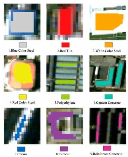
Figure 1.
Nine classes of selected samples in remote sensing image.

Table 1.
Reference classes and sizes of training and testing set of our data.
Indian Pines (IP) data set consists of 145 × 145 pixels with 224 bands ranging from 0.4 to 2.5 micrometers. In IP data set, labelled samples are split into the training, test, and validation set with the ratio of 1.5:1.5:7.
2.2. Input of BRI-CNN
The input images are created with every single pixel and its eight neighbourhoods, and a set of 9 × 9 images is formed. With a pixel and its neighbourhoods, we classify the pixel using the texture information between the pixel and its neighbours. However, there are 64 bands in our HSI data that ordinarily would be correlated [35]. So instead taking the original image as input, we decomposed these bands into a set of linearly uncorrelated principal components using PCA. By decreasing the dimension of the whole image, we can reduce the time complexity and accelerate the convergence of our algorithm. Assuming that the spectral features of any two land-cover types differ from each other more than 1%, we retained 99% of the variance. Finally, 5 principal components in our data set and 24 in IP data set were retained; thus, the input data is an aggregation of 9 × 9 × 5 images for our data set and 9 × 9 × 24 for IP data set. Note that if the network is applying to another different hyperspectral image, the input should be adjusted according to the result of PCA.
2.3. Main Structure of a Conventional CNN
Each input image is fed into a layer of convolutional kernels, which is actually a set of matrices. They convolve with the input image according to Equation (1), and the result z is then activated by an activation function as Equation (2):
where W is the kernel matrix; a is the input image, and b is called the bias term. Rectified Linear Units (ReLU), a nonlinear activation function, is chosen in our study. This function allows a network to easily obtain sparse representations, which increases with sparsity-including regularization [36]. Besides, the ReLU function avoids the vanishing gradient [37] and exploding gradient problems.
After the activation, local primary features are extracted and mapped into a set of intermediate patches (known as feature maps), which can be regarded as the input images of the next convolutional layer. A convolution and an activation operation as a basic process, repeating for certain times, stops until the whole feature map can be covered by the convolutional kernel. It is believed that features in all depths can be extracted after that.
Outcomes of the last convolutional layer are flattened to a column of neurons and each neuron contains a value that represents a feature of the original input image. To calculate the similarity between these values and the label of their original input image, neurons are connected to Fully Connected (FC) layers, in which neuron features are correlated and finally we can get another set of neurons according to their correlations. The Normalized Exponential Function, also known as the Softmax Function [38], is a generalization of the logistic function to a multiclass classification problem. The possibility q that one input image belongs to each selected class is calculated using Equation (3):
where represents one value from the neurons of the output layer; i represents the number of one class; K is the total number of classes.
Obviously, because the values of kernels and neurons are initialized manually, the predicted label may be far from the correct. Therefore, a Cross Entropy loss function is utilized to express the discrepancies between calculated and true labels in most cases. Taking p as the true label distribution, the cross entropy over a given set is defined as follows (Equation (4)):
The loss will propagate backward to adjust the weights of kernels and neurons. Once we diminish the loss, i.e., discrepancy between calculated and true label, the capability of the network increases.
From the first convolutional operation to the tuning of weights, the whole procedure constitutes the training process in CNN. Adequate number of manual labelled input images helps the model to learn sufficient features of different land-cover types. After the training process ceases, a predicted process is followed, during which all weights in the model are invariant and the type of unknown input images can be predicted.
2.4. Structure of BRI-CNN
Rather than one specific size of a convolutional kernel, we used three different scale kernels (1 × 1, 3 × 3, and 5 × 5) simultaneously to extract different kinds of features in the input images. 3 × 3 kernels are for edge spatial features, the 5 × 5 are for adjacency spatial features, and the 1 × 1 aim to extract interior spectral features, making it possible to adjust feature proportions later on.
After the convolution processes, we stacked different outcomes and flattened them into one-dimension, regarded as the input of the sub-sequential fully connected layer. The last part of our CNN is a classifier, which classifies a pixel while predicting and performing back-propagation while training. The detailed structure of the tuned model is shown in Figure 2 and Table 2.
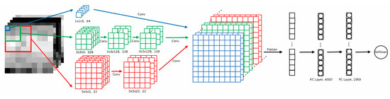
Figure 2.
Diagram of the proposed CNN structure.
Table 2.
Detailed structure of the proposed model.
All hyper-parameters in our model, including the size of kernels, the number of kernels in convolutional layers, etc., were determined after near one hundred times of tests. We used 64 1 × 1 × 5 kernels on input image to get the first set of feature maps, 128 3 × 3 × 5 kernels followed by two layers with 128 3 × 3 × 128 kernels to get the second set of feature maps, and 22 5 × 5 × 5 kernels followed by one layer with 22 5 × 5 × 22 kernels to get the third set of feature maps. Same padding ensured that three sets of feature maps had the same size in spatial dimension; thus, we stacked them in a spectral dimension. Two fully connected layers have 4000 and 1000 neurons, respectively. The number of neurons in the output layer is determined by the number of labelled classes in the training data set. When applied in our data set, the output layers have ten neurons with a softmax activation function.
2.5. Optimization Function
In our experiment, we use Adadelta to minimize the loss. Adadelta is an adaptive gradient descent optimization algorithm, which uses first order methods to simulate second order derivatives in Newton’s method [38]. The weight of the neurons is updated as follows (Equations (5)–(8)):
where E is the expected value; g is the gradient of the loss function; is a constant momentum factor; RMS means root mean square; represents the updated value. Compared with other optimizers, Adadelta relies slightly on hyper-parameters and causes the loss function to converge very rapidly at the beginning of the training. At the end of the training process, the loss fluctuates slightly over the minimum value.
As mentioned above, we calculate the partial derivative of the loss function, while optimizing the weight, as follows (Equation (9)):
Clearly, the partial derivative of Equation (4) is easy to compute when applying Softmax Function (Equation (3)). Thus, the time complexity is reduced.
2.6. Evaluation Method
Evaluation methods for deep learning always describe the global condition, such as accuracy and loss. They are good indicators over the whole image, but global accuracy cannot represent the true accuracy within a selected area. To be more precise, we compared the predicted outcome with the result of manual interpretation in the same selected area and then calculated the Prediction Accuracy (PA), which is the most accurate criterion within a specific area. In addition, we divided the error into False Negative Rate (FNR) and False Positive Rate (FPR), which are convenient for reducing the error and improving the network in two different ways.
Given FN and FP as the number of unrecognized pixels and wrongly recognized pixels, PA, FNR and FPR are computed as follows:
where M and N are the width and height of the selected area, respectively.
3. Results and Discussion
To better extract the interior-edge-adjacency features and classify the building roof, we tuned different hyper-parameters independently, and obtained the most effective structure for the network. In our experiment, four typical areas where the PA is relatively low are selected to analyse in detail.
3.1. Size of Convolutional Kernels
The discussion of the size of convolutional kernels is divided into two parts: the convolutional kernels associated with spatial information and the convolutional kernels related to spectral features. Taking into consideration the high resolution of this image and the usual simple shape of the constructions, we chose small scale kernels to extract textural features. Other spatial features, for example, semantic features, were extracted by larger kernels (e.g., 7 × 7). However, because 7 × 7 kernels are so large it is difficult for the network to converge. By segmenting large kernels into smaller ones, the computational cost can be reduced [39]. In the edges of building rooftops, smaller scale kernels perform much better than the larger ones. Thus, to integrally recognize buildings we tried 2 × 2 kernels, 3 × 3 kernels and 5 × 5 kernels separately, using the network of BRI-CNN, instead of using three different size kernels simultaneously.
As shown in Figure 3, our proposed network, although performing better near the edges, cannot separate elongated building rooftops only using 3 × 3 kernels (Figure 3c) and performs even worse using 2 × 2 kernels (Figure 3d), which means that, as the size of the convolutional kernels becomes smaller, the network is even worse in separating the edge features of building rooftops. But moderate quantities of large-scale kernels (e.g., 5 × 5) help to separate adjacent buildings (Figure 3b), indicating 5 × 5 kernels can highlight the adjacency spatial features. As seen from the curves (Figure 3e–g), the loss functions have already converged within 150 epochs. Thus, we ceased the training processes after 150 epochs and acquired well trained models. Training accuracies of the three kernels (5 × 5, 3 × 3, and 2 × 2) are about 99.49%, 99.31% and 99.42%, respectively. By using the Adadelta Optimizer, accuracies fluctuate around the global minimum values. Additionally, to evaluate these three kernels more precisely, we also calculate Prediction Accuracy, False Negative Rate, and False Positive Rate. As shown in Table 3, for FPR and PA, the kernel size of 5 × 5 shows much higher than that of the 3 × 3 kernels and 2 × 2 kernels. But with the 3 × 3 kernels, there is a much lower cost in the false negative rate. So to combine the advantage of 3 × 3 and 5 × 5 kernels, we used both in parallel.
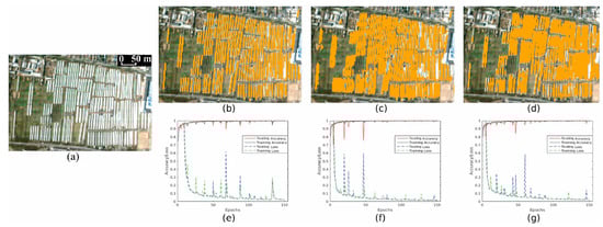
Figure 3.
The proposed network outcomes using three different scale kernels separately. (a): a part of original image with building rooftops made by White Colour Steel. (b): the predicted output that only using 5 × 5 kernels, while (c) using 3 × 3 kernels and (d) using 2 × 2 kernels. (e–g): accuracies and loss curves of training and testing of (b–d).
Table 3.
Seven different criteria on the network using three different scale kernels.
After determining the size of convolutional kernels about spatial information, we added to the model 1 × 1 kernels, the key part of BRI-CNN, which have a strong response to interior spectral features of building roof. As shown in Figure 4, it is much more difficult for a model without 1 × 1 kernels to recognize pixels located in the interior of a building. Figure 4d is a perfect match with the ground truth, whereas Figure 4c, obviously, is unqualified. Possible reasons are the input images formed by inner pixels and their neighbours have no texture features, and normal convolutional kernels are mainly used to extract texture features whereas inter-channel features are weakened. The use of 1 × 1 convolutional kernels can strengthen inter-channel features or interior features, so three scale convolutional kernels are employed simultaneously.
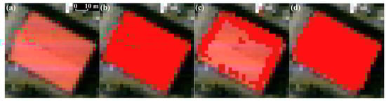
Figure 4.
Different outcomes of structures with and without 1 × 1 kernels. (a) a part of original image that having Red Tile land-cover type. (b) the Ground Truth (GT) of this building, (c) the prediction outcome of the model without 1 × 1 convolutional kernel. (d) the outcome generated by the network with 1 × 1 convolutional kernels.
3.2. Number of Convolutional Kernels
There are three different kernel sizes: 1 × 1, 3 × 3 and 5 × 5. As mentioned above, 1 × 1 kernels are used to extract the spectral features within channels. Because of its limited field of view, this kernel size does not contribute to the extraction of spatial features. Larger scale kernels are used to extract spatial features, including edge and adjacency features. However, the larger the scale of kernel, the more difficult the network is to converge. So we cut down the number of 5 × 5 kernels and increased the number of 3 × 3 kernels, but still maintained moderate quantities of 5 × 5 kernels to split small adjacent buildings. The minimum number of 5 × 5 convolutional kernels is 22; fewer than this number will influence the performance of extracting small buildings. After a series of tests, we chose 64 1 × 1 kernels, 128 3 × 3 kernels and 22 5 × 5 kernels.
As shown in Figure 5, the edges of building rooftops are not recognized in Figure 5c, but the building rooftops are almost completely extracted in Figure 5d. As shown in Table 4, the model with 128 3 × 3 kernels performs much better at the edge of the building roof than that with 32 3 × 3 kernels. More precisely, the FNR of the former is seven times lower than the latter.
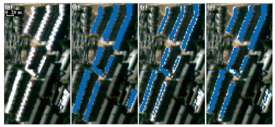
Figure 5.
Results of networks using different 3 × 3 kernel number. (a) a part of original image where the building roofs are made of Ceram. (b) the reference building roofs. (c) the output of the network using 32 3 × 3 convolutional kernels and 22 5 × 5 convolutional kernels, (d) the output using 128 3 × 3 kernels and 22 5 × 5 convolutional kernels.
Table 4.
Seven criteria on two network structures with different 3 × 3 kernel numbers.
In addition, we also investigated the outputs of models with different 1 × 1 kernel numbers. For the 1 × 1 kernel, with 16 kernels, 32 kernels, 48 kernels, and 64 kernels, we obtained PA of 87.42%, 89.71%, 94.33%, and 98.84%, respectively. Beyond the threshold of 64–80 kernels, the PA tends to be steady. The relation between the number of 1 × 1 kernels and accuracy is shown in Figure 6.
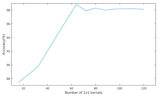
Figure 6.
Accuracies of models with different numbers of 1 × 1 convolutional kernels in a selected area.
3.3. Number of Convolutional Layers
The deeper the convolutional layers, the more sophisticated the extracted features. Lin, Chen, and Yan [40] called 1 × 1 kernel network in network; one layer of 1 × 1 kernels sufficient to extract all the features within the channels. Additional 1 × 1 convolutional layers will result in wasted computation. According to [39], one layer of large kernels can be separated into several layers of smaller kernels. For example, three consecutive layers of 3 × 3 kernels extract the same quantity of features as one layer of 7 × 7 kernels; two layers of 5 × 5 kernels extract features in a like manner. That is why we replaced one layer of large size kernels with more than one layers of small size kernels. Finally, the proposed model was constructed with one 1 × 1 convolutional layer, three 3 × 3 convolutional layers, and two 5 × 5 convolutional layers.
3.4. Number of Fully Connected Layers and Neurons
Convolutional layers are used to map raw data in feature space, indicating that CNNs learn different kinds of building features by convolutional layers. After extracting features, we combined different features. Different combinations of features represent different kinds of buildings. Fully connected layers integrate features and map different feature combinations into label space. Since the same padding is applied after every convolution operation, and the strides of convolutional kernels are 1, we obtain 64, 128, and 22 7 × 7 feature maps in 1 × 1, 3 × 3, and 5 × 5 branches after convolving, respectively. We stacked them in the channel dimension and attained a 214 × 7 × 7 feature map, which, when flattened, resulting in a one-dimensional vector as the input layer for sub-sequential fully connected layers. The number of input neurons for fully connected layers is 10,486. Thus, we tried different quantities of fully connected layers and neurons. Finally, we determined a two-FC-layer structure, with 4000 neurons in one layer and 1000 neurons in the other layer.
In Figure 7, multiple different architectural materials are shown. Although in Figure 7b all buildings are recognized, some other pixels are mistakenly regarded as architectural materials. As indicated in Table 5, the FPR corresponding to Figure 7b is high, which subsequently leads to a low PA. Thus, we simplified the structure of the FC layers as shown in Figure 7c–e and attained the lowest FPR and highest PA in Figure 7e. Meanwhile, this structure maintained a low FNR.
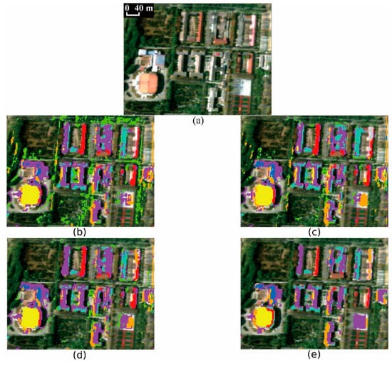
Figure 7.
Different outcomes of four different fully connected structures. (a) a part of original image. (b–e) outputs of structures with different amounts of FC layers or neurons in each FC layer. (b) with three FC layers and 8000, 4000, 1000 neurons in each layer, (c) with three layers and 4000, 1000, 200 neurons in each layer, (d) with two layers and 6000, 2000 neurons in each layer, (e) with two layers and 4000, 1000 neurons in each layer.
Table 5.
PA, FNR, FPR of four different fully connected structures.
3.5. Performance on Public Data Sets
We briefly discussed the above processes using the IP data set, especially the size of convolutional kernels in Section 3.1, the number of kernels in Section 3.2, and the number of FC layers in Section 3.4. Six models with different sizes of kernels in convolutional layers were trained on the IP data set to research the dependency of recognition results on the kernel size. Prediction accuracies, together with the Cohen’s kappa coefficients () [41] of the results of these models were listed in Table 6. It shows a general increase in AA (Average Accuracy), OA (Overall Accuracy) and , with the increasing size of kernels, partly because of the extending field of view.
Table 6.
Classification results of Indian pines data set using different kernel sizes.
Besides, seven different models were applied on the IP data set, which were identical to those mentioned in Section 2.4, except for the number of 1 × 1 or 3 × 3 kernels. The Classification results can be seen in Table 7. What we can learn from these results is that the capability of BRI-CNN will be strengthened by adding the numbers of 1 × 1 and 3 × 3 kernels to some extent.
Table 7.
Classification results of Indian pines data set using different kernel numbers.
To highlight the importance of the 1 × 1 kernels, we implemented an experiment without them while keeping all other hyper-parameters unchanged. The experimental results show that, with 64 1 × 1 kernels, CNN can get nearly 2% higher OA and 0.01 higher during predicting. All models above were trained with the training, test, and validation ratio of 1.5:1.5:7.
3.6. Comparisons with Other Models
As we applied our model into IP data set, a validation data set for most DL models in the HSI domain, we can compare our model with other previous works. As seen in Table 8, a comparison of six outputs of different models shows that BRI-CNN generally performs better than the other four state-of-the-art models. Compared with the best model [34], our proposed network attains an OA that is 0.24% higher.
Table 8.
Classification results of Indian pines data sets using different models.
Figure 8a–c show the outcomes of ground-truth labels, SSRN [29] and BRI-CNN. Figure 8d–f show a representative area in the left of original figures. In Figure 8e, boundary pixels between the mainland-cover types are irregular, whereas in Figure 8f, the boundaries of large pieces are in alignment, which is more similar to Figure 8d.
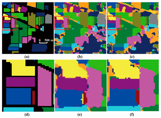
Figure 8.
Comparisons of true labels and two different outputs. (a) Ground-truth labels. (b) Result of SSRN from [29]. (c) Result of BRI-CNN. (d,e,f) Segments of outputs in ground-truth, SSRN (from [29]), and BRI-CNN, respectively.
4. Conclusions
In this paper, we presented a new approach to combine interior, edge, and adjacency features using multi-scale kernels in parallel. The key structure of BRI-CNN is a set of 1 × 1 convolutional kernels, which is proved to be a great improvement in recognizing types of land-cover, including building roof, due to the interior spectral features. It was found that 3 × 3 kernels work well at the edge of building roof and 5 × 5 kernels are efficient to separate adjacent buildings. Using these three different scale kernels, the proposed network can perform robust both near the boundary and in the interior of building roof. The experimental results indicate that the BRI-CNN model achieves nearly 0.2% higher overall accuracy and average accuracy than that of SSRN model, and at least 1% higher than most models, including conventional CNN and DBN models. Besides all the hyper-parameters discussed above, we found input size is also a factor that affects the subsequent structure. As the input size increases, more features are included in one input picture, making it much more difficult to train the networks with little improvement. In addition, when building roofs are smaller than the size of the convolutional kernel, we should pay attention to the extracting result, because it may be terrible.
Author Contributions
Conceptualization, C.Y.; Methodology, C.Y., H.L. and X.L.; Formal Analysis, C.Y., C.L. and X.L.; Writing—Original Draft Preparation, H.L., C.L. and X.L.; Writing—Review & Editing, C.Y., Y.L., J.L., W.N.G. and J.M.J.; All authors have read and agreed to the published version of the manuscript.
Funding
This research was funded by the National Natural Science Foundation of China, grant number 42071411 and the Second Tibetan Plateau Scientific Expedition and Research Program (STEP), grant number 2019QZKK0902.
Institutional Review Board Statement
Not applicable.
Informed Consent Statement
Not applicable.
Data Availability Statement
The data are not publicly available due to privacy issues.
Conflicts of Interest
The authors declare no conflict of interest.
References
- Wang, R.; Nie, F.; Yu, W. Fast Spectral Clustering with Anchor Graph for Large Hyperspectral Images. IEEE Geosci. Remote Sens. Lett. 2017, 14, 2003–2007. [Google Scholar] [CrossRef]
- Wentz, E.A.; Anderson, S.; Fragkias, M.; Netzband, M.; Mesev, V.; Myint, S.W.; Quattrochi, D.; Rahman, A.; Seto, K.C. Supporting Global Environmental Change Research: A Review of Trends and Knowledge Gaps in Urban Remote Sensing. Remote Sens. 2014, 6, 3879–3905. [Google Scholar] [CrossRef] [Green Version]
- Ye, C.M.; Cui, P.; Pirasteh, S.; Li, J.; Li, Y. Experimental approach for identifying building surface materials based on hyperspectral remote sensing imagery. J. Zhejiang Univ. Sci. A 2017, 18, 984–990. [Google Scholar] [CrossRef]
- Lu, B.; Dao, P.D.; Liu, J.; He, Y.; Shang, J. Recent advances of hyperspectral imaging technology and applications in agriculture. Remote Sens. 2020, 12, 2659. [Google Scholar] [CrossRef]
- Pontius, J.; Martin, M.; Plourde, L.; Hallett, R. Ash decline assessment in emerald ash borer-infested regions: A test of tree-level, hyperspectral technologies. Remote Sens. Environ. 2008, 112, 2665–2676. [Google Scholar] [CrossRef]
- Prasad, S.; Bruce, L.M. Limitations of Principal Components Analysis for Hyperspectral Target Recognition. IEEE Geosci. Remote Sens. Lett. 2008, 5, 625–629. [Google Scholar] [CrossRef]
- Li, J.; Bioucas-Dias, J.M.; Plaza, A. Hyperspectral Image Segmentation Using a New Bayesian Approach With Active Learning. IEEE Trans. Geosci. Remote Sens. 2011, 49, 3947–3960. [Google Scholar] [CrossRef] [Green Version]
- Li, W.; Prasad, S.; Fowler, J.E.; Bruce, L.M. Locality-Preserving Dimensionality Reduction and Classification for Hyperspectral Image Analysis. IEEE Trans. Geosci. Remote Sens. 2012, 50, 1185–1198. [Google Scholar] [CrossRef] [Green Version]
- Melgani, F.; Bruzzone, L. Classification of hyperspectral remote sensing images with support vector machines. IEEE Trans. Geosci. Remote Sens. 2004, 42, 1778–1790. [Google Scholar] [CrossRef] [Green Version]
- Merenyi, E.; Farrand, W.H.; Taranik, J.V.; Minor, T.B. Classification of hyperspectral imagery with neural networks: Comparison to conventional tools. Eurasip. J. Adv. Signal Process. 2014, 2014, 71. [Google Scholar] [CrossRef] [Green Version]
- Bioucas-Dias, J.M.; Plaza, A.; Dobigeon, N.; Parente, M.; Du, Q.; Gader, P.; Chanussot, J. Hyperspectral Unmixing Overview: Geometrical, Statistical, and Sparse Regression-Based Approaches. IEEE J. Sel. Top. Appl. Earth Obs. Remote Sens. 2012, 5, 354–379. [Google Scholar] [CrossRef] [Green Version]
- Bo, D.; Zhang, L. A Discriminative Metric Learning Based Anomaly Detection Method. IEEE Trans. Geosci. Remote Sens. 2014, 52, 6844–6857. [Google Scholar]
- Gu, Y.; Chanussot, J.; Jia, X.; Benediktsson, J.A. Multiple Kernel Learning for Hyperspectral Image Classification: A Review. IEEE Trans. Geosci. Remote Sens. 2017, 55, 6547–6565. [Google Scholar] [CrossRef]
- Sigurdsson, J.; Úlfarsson, M.Ö.; Sveinsson, J.R. Semi-Supervised Hyperspectral Unmixing. In Proceedings of the 2014 IEEE International Geoscience and Remote Sensing Symposium, Quebec, QC, Canada, 13–18 July 2014. [Google Scholar]
- Wang, T.; Zhang, H.; Hui, L.; Jia, X. A Sparse Representation Method for a Priori Target Signature Optimization in Hyperspectral Target Detection. IEEE Access 2017, 6, 3408–3424. [Google Scholar] [CrossRef]
- Fan, Z.; Bo, D.; Zhang, L.; Zhang, L. Hierarchical feature learning with dropout k -means for hyperspectral image classification. Neurocomputing 2016, 187, 75–82. [Google Scholar]
- Haut, J.M.; Paoletti, M.; Plaza, J.; Plaza, A. Cloud implementation of the K-means algorithm for hyperspectral image analysis. J. Supercomput. 2017, 73, 1–16. [Google Scholar] [CrossRef]
- Lv, X.; Ming, D.; Chen, Y.Y.; Wang, M. Very high resolution remote sensing image classification with SEEDS-CNN and scale effect analysis for superpixel CNN classification. Int. J. Remote Sens. 2019, 40, 506–531. [Google Scholar] [CrossRef]
- Huang, G.; Liu, Z.; Weinberger, K. Densely Connected Convolutional Networks. In Proceedings of the IEEE Conference on Computer Vision and Pattern Recognition, Las Vegas, NV, USA, 27–30 June 2016. [Google Scholar]
- Sabour, S.; Frosst, N.; Hinton, G. Dynamic Routing Between Capsules. arXiv 2017, arXiv:1710.09829. [Google Scholar]
- Cao, J.; Zhao, C.; Wang, B. Deep Convolutional networks with superpixel segmentation for hyperspectral image classification. In Proceedings of the 2016 IEEE International Geoscience and Remote Sensing Symposium (IGARSS), Beijing, China, 10–15 July 2016. [Google Scholar]
- Yu, S.; Jia, S.; Xu, C. Convolutional neural networks for hyperspectral image classification. Neurocomputing 2016, 219, 88–98. [Google Scholar] [CrossRef]
- Zhao, W.; Du, S. Learning multiscale and deep representations for classifying remotely sensed imagery. ISPRS Photogra. Remote Sens. 2016, 113, 155–165. [Google Scholar] [CrossRef]
- Shi, C.; Pun, C.M. Superpixel-based 3D Deep Neural Networks for Hyperspectral Image Classification. Pattern Recogn. 2017, 74, S0031320317303515. [Google Scholar] [CrossRef]
- Nogueira, K.; Penatti, O.A.B.; Santos, J.A. Dos Towards Better Exploiting Convolutional Neural Networks for Remote Sensing Scene Classification. Pattern Recogn. 2016, 61, 539–556. [Google Scholar] [CrossRef] [Green Version]
- Chen, Y.; Zhao, X.; Jia, X. Spectral–Spatial Classification of Hyperspectral Data Based on Deep Belief Network. IEEE J. Sel. Top. Appl. Earth Obs. Remote Sens. 2015, 8, 2381–2392. [Google Scholar] [CrossRef]
- Paoletti, M.; Haut, J.; Plaza, J.; Plaza, A. Deep\&Dense Convolutional Neural Network for Hyperspectral Image Classification. Remote Sens. 2018, 10, 1454. [Google Scholar] [CrossRef] [Green Version]
- Chen, X.; Xiang, S.; Liu, C.-L.; Pan, C.-H. Vehicle Detection in Satellite Images by Hybrid Deep Convolutional Neural Networks. Geosci. Remote Sens. Lett. IEEE 2014, 11, 1797–1801. [Google Scholar] [CrossRef]
- Zhong, Z.; Li, J.; Luo, Z.; Chapman, M. Spectral-Spatial Residual Network for Hyperspectral Image Classification: A 3-D Deep Learning Framework. IEEE Trans. Geosci. Remote Sens. 2018, 56, 847–858. [Google Scholar] [CrossRef]
- He, K.; Zhang, X.; Ren, S.; Sun, J. Deep Residual Learning for Image Recognition. In Proceedings of the 2016 IEEE Conference on Computer Vision and Pattern Recognition (CVPR), Las Vegas, NV, USA, 27–30 June 2016; IEEE Computer Society: Los Alamitos, CA, USA, 2016; pp. 770–778. [Google Scholar]
- Gao, Q.; Lim, S.; Jia, X. Hyperspectral Image Classification Using Convolutional Neural Networks and Multiple Feature Learning. Remote Sens. 2018, 10, 299. [Google Scholar] [CrossRef] [Green Version]
- Li, Y.; Xie, W.; Li, H. Hyperspectral image reconstruction by deep convolutional neural network for classification. Pattern Recogn. 2017, 63, 371–383. [Google Scholar] [CrossRef]
- Chen, Y.; Jiang, H.; Li, C.; Jia, X.; Ghamisi, P. Deep Feature Extraction and Classification of Hyperspectral Images Based on Convolutional Neural Networks. IEEE Trans. Geosci. Remote Sens. 2016, 54, 6232–6251. [Google Scholar] [CrossRef] [Green Version]
- Paoletti, M.E.; Haut, J.M.; Fernandez-Beltran, R.; Plaza, J.; Plaza, A.; Li, J.; Pla, F. Capsule Networks for Hyperspectral Image Classification. IEEE Trans. Geosci. Remote Sens. 2018, 57, 2145–2160. [Google Scholar] [CrossRef]
- Hotelling, H. Analysis of a complex of statistical variables into principal components. J. Educ. Psychol. 1933, 24, 417–441, 498–520. [Google Scholar] [CrossRef]
- Glorot, X.; Bordes, A.; Bengio, Y. Deep Sparse Rectifier Neural Networks. In Proceedings of the 14th International Conference on Artificial Intelligence and Statistics, Fort Lauderdale, FL, USA, 11–13 April 2011; Volume 15, pp. 315–323. [Google Scholar]
- Kolen, J.F.; Kremer, S.C. Gradient Flow in Recurrent Nets: The Difficulty of Learning LongTerm Dependencies. In A Field Guide to Dynamical Recurrent Networks; IEEE; Wiley-IEEE Press: Piscataqay, NJ, USA, 2001; ISBN 9780470544037. [Google Scholar]
- Bishop, C.M. Pattern Recognition and Machine Learning (Information Science and Statistics); Springer: Berlin/Heidelberg, Germany, 2006. [Google Scholar]
- Szegedy, C.; Vanhoucke, V.; Ioffe, S.; Shlens, J.; Wojna, Z. Rethinking the Inception Architecture for Computer Vision. In Proceedings of the CVPR, Las Vegas, NV, USA, 27–30 June 2016. [Google Scholar]
- Lin, M.; Chen, Q.; Yan, S. Network In Network. arXiv 2013, arXiv:1312.4400. [Google Scholar]
- Cohen, J. A Coefficient of Agreement for Nominal Scales. Educ. Psychol. Meas. 1960, 20, 37–46. [Google Scholar] [CrossRef]
Publisher’s Note: MDPI stays neutral with regard to jurisdictional claims in published maps and institutional affiliations. |
© 2021 by the authors. Licensee MDPI, Basel, Switzerland. This article is an open access article distributed under the terms and conditions of the Creative Commons Attribution (CC BY) license (https://creativecommons.org/licenses/by/4.0/).