Article

A Spatio-Temporal Brightness Temperature Prediction Method for Forest Fire Detection with MODIS Data: A Case Study in San Diego

1
State Key Laboratory of Remote Sensing Science, Beijing Normal University, Beijing 100875, China
2
Beijing Key Laboratory of Environmental Remote Sensing and Digital City, Beijing Normal University, Beijing 100875, China
3
Faculty of Geographical Science, Beijing Normal University, Beijing 100875, China
4
State Key Laboratory of Resources and Environment Information System, Institute of Geographic Sciences and Natural Resources Research, Chinese Academy of Sciences, Beijing 100101, China
5
University of Chinese Academy of Sciences, Beijing 100049, China
*
Author to whom correspondence should be addressed.
Remote Sens. 2021, 13(15), 2900; https://doi.org/10.3390/rs13152900
Submission received: 19 June 2021 / Revised: 20 July 2021 / Accepted: 21 July 2021 / Published: 23 July 2021

Abstract

:
Early detection of forest fire is helpful for monitoring the spread of fire promptly, minimizing the loss of forests, wild animals, human life, and economy. The performance of brightness temperature (BT) prediction determines the accuracy of fire detection. Great efforts have been made on BT prediction model building, but there still remains some uncertainty. Based on the widely used contextual BT prediction model (CM) and temporal-contextual BT prediction model (TCM), we proposed a spatio-temporal contextual BT prediction model (STCM), which involves historical images to contrast the BT correlation matrix between the pixel to be predicted and its background pixels within a dynamic window, and the spatial distance factor was introduced to modify the BT correlation matrix. We applied the STCM to a fire-prone area in San Diego, California, US, and compared it with CM and TCM. We found that the average RMSE of STCM was 12.54% and 9.12% lower than that of CM and TCM, and the standard deviation of RMSE calculated by STCM was reduced by 12.04% and 15.57% compared with CM and TCM, respectively. In addition, the bias of STCM was concentrated around zero and the range of bias of STCM was 88.7% and 15.3% lower than that of CM and TCM, respectively. The results demonstrated that the STCM can be used to obtain the highest BT prediction accuracy and most robust performance, followed by TCM, and CM performed worst. Our research on the BT prediction of potential fire pixels is helpful for improving the fire detection accuracy and is potentially useful for the prediction of other environmental variables with high spatial and temporal autocorrelation. However, the requirement of high-quality continuous data will limit the application of STCM in cloudy and rainy areas.

Graphical Abstract

1. Introduction

Forest fires destroy millions of hectares of the worldwide forests every year [1], causing environmental, social, and economic damages and loss of life [2,3,4]. In the last few decades, wildfire activities increased significantly in many areas of the world because of the rise in temperatures and human activities [5,6,7]. Satellite remote sensing is efficient for fire detection [3], which can monitor and map the spatial and temporal distribution of forest fires accurately and timely [8], thus providing valuable information at a global scale and generally at low costs [3], such as NOAA/AVHRR, EOS/MODIS, MSG/SEVIRI, HJ-1B/IRS, Landsat TM/ETM+, ASTER, Sentinel, etc. However, the fire detection algorithm and fire data are still on the way. Thermal landscape heterogeneity caused by forest fires shows high spatial variability and high temporal variability, while existing sensors have limitations in providing TIR data of global land with both high spatial and temporal resolution [9]. Terra/Aqua-moderate resolution imaging spectroradiometer (MODIS) data have been widely used for forest fire monitoring because of their high radiometric resolution, the trade-off between spatial and temporal resolution modes, and a high saturation level. Abundant fire detection products derived from MODIS, including global daily active fire product version 4 (MOD14) with fewer saturated pixels at 1-km resolution [10], monthly burned area product (MCD45) at 500-m resolution [11], and biomass burning emission product [12], have become an important source of information for fire science and management [13,14,15,16].
A contextual fire detection algorithm used in the MOD14 products identifies a pixel as a “potential fire pixel” with a series of thresholds for reflection and radiance and detects the “relative fire pixel” with a threshold of the difference between the observed brightness temperature (BT) and the prediction BT of the potential fire pixel. Finally, false alarms are rejected by using a series of thresholds for the view and solar zenith angles, the number of neighboring pixels excluded as water or background fires, etc., [9]. The predicted BT value of the potential fire pixel represents the trend of the BT of the pixel under the steady thermal landscape without a forest fire, land cover change, or human activities. If the true BT of the pixel is greater than the predicted BT and the difference between two values exceeds the predetermined threshold, this pixel is considered a “relative fire pixel” or “real fire pixel”. Therefore, the BT prediction of the potential fire pixel is a crucial step in fire monitoring and the prediction accuracy of the BT of the potential fire pixel determines the detection accuracy of the relative fire pixel.
At present, the BT prediction techniques could be summarized in three main categories: contextual model (CM), multi-temporal model (TM), and spatio-temporal model (STM). CM predicts the BT (in channels centered at 4.0 and 11.0 μm) of potential fire pixels by averaging its non-fire background BTs within a window [17,18], and the maturity of the CM is evidenced by the large number of citations and data applications found in the literature [19,20,21]. However, the CM does not take advantage of multi-temporal information, which exhibits huge potential in prediction of thermal landscapes [22]. TM predicts the BT of the potential fire pixel according to its historical BT time series. For example, Laneve et al. modelled the natural variation of the surface temperature to detect change using diurnal and nocturnal SEVIRI images [23]. Roberts et al. proposed a diurnal temperature cycle model (DTC) to predict the BT of the fire pixel based on historical multi-temporal infrared images, which allowed the fire pixel to be detected [24]. Su predicted the BT of the fire pixel by using a temporal fitting model (BFAST) based on time series data, which allowed the fire pixels to be identified [25]. The result demonstrated that the detection accuracy of fire pixels has a significant increase with time series data involved. Mazzeo et al. proposed an index called Absolute Local Index of Change of the Environment (ALICE) to detect anomaly value of the BT in the MIR band by comparing observed value with the predicted value, which computed by averaging the long-term satellite records [3]. Although these TMs can detect fire pixels at an early period, missing pixel values will affect the BT prediction accuracy. Moreover, TM ignores the strong correlation between the potential fire pixel and its surrounding pixels. STM predicts the BT of the fire pixel according to the historical BT of the fire pixel and its surrounding pixels, which involves both the multi-temporal information and spatial neighborhood information in the prediction. For example, Pavlidou et al. constructed a normalized BT prediction model of the central pixels by dividing the average value of their neighboring pixels, and then the anomaly pixels were identified by moving a temporal window within a specific period. The algorithm can highlight short-term, localized, non-periodic fluctuations [26]. Lei Lin et al. proposed a temporal-contextual model (TCM) that used the strong correlation between the central pixel and its neighborhood, calculated using time series data to predict the BT of the fire pixel, which can obtain a higher fire detection accuracy than the contextual algorithm [27]. However, the same weights assigned to all neighborhood pixels in TCM may cause prediction errors because the neighborhoods within a given window have differentiated contributions to the BT prediction of the central pixel. Additionally, a large, fixed window is used in TCM to obtain enough valid background pixels for data with different quality; however, the fixed window leads to redundant neighborhood information for high-quality data, which makes TCM inefficient.
To address the above issues, this work proposed a spatio-temporal contextual BT prediction model (STCM) for fire detection that corrected the contribution of different background pixels to the prediction of the pixel to be determined in TCM by adding a distance factor to the BT correlation matrix, which describes the relationship between the central pixel with its background pixels. Additionally, a dynamic window that used to select valid background pixel was employed in STCM to improve the efficiency of the method. We tested it in a study area of San Diego in Southern California, America. The predicted BT was evaluated by comparing with the contextual algorithm (CM) and the temporal–contextual algorithm (TCM).

2. Materials

2.1. Study Area

San Diego is on the coast of the Pacific Ocean in Southern California with an area of approximately 963 km2, approximately 190 km south of Los Angeles, and immediately adjacent to the border with Mexico. Characterized by the semi-arid climate [28,29] or a Mediterranean climate [30,31], the study area has warm, dry summers and mild winters with an average of 201 days above 21 °C and low rainfall (230–330 mm annually [32]). The climate in San Diego often varies significantly over short geographical distances, resulting in microclimates. San Diego is a forest fire disaster-prone area. According to the EM-DAT (The International Disasters Database, http://www.emdat.be/about, accessed on 19 June 2021), recorded from 1900 to 2016, there were a total of 78 forest fires in America, of which, California had a total of 41 and San Diego had a total of 8, causing total deaths of 17, total affected area of 650,000 km2, and economic losses of $3.7 billion. As a fire-prone area, it is necessary to perform the accurate BT prediction to improve the accuracy of early fire detection. San Diego suffered the most serious forest fires on 21 October 2007 (Figure 1).

2.2. Data and Data Preprocessing

Daily MODIS Level 1B product with spatial resolution of 1 km from 22 August 2007 to 22 October 2007 (MOD02 and MOD03 geolocation data with a total of 62 groups) and the MODIS global land cover product (MOD12Q1) were used in this study. MOD02 data sets use the Swath data type to record two calibrated data products: the reflectance and radiance of 36 bands. These data can be downloaded from the Level-1 and Atmosphere Archive & Distribution System (LAABS) Distributed Active Archive Center (DAAC) (http://ladsweb.modaps.eosdis.nasa.gov/search/order/1/MODIS:Terra,MODIS:Aqua, accessed on 19 June 2021). Table 1 shows the band features and its application of MOD02 data.
The preprocessing procedure for MODIS data includes the following processes: geometric calibration, cutting out the study area, quality checking, reflectance calculation, BT inversion, and the input data extraction of STCM model. The MODIS Reprojection Tool Swath (MRT Swath), combined with MOD03 data, was used to convert the map projection from Integerized Sinusoidal to Albers, transfer the data type from .hdf to .tif, and remove “bowtie effect” of the MOD02 data [33]. Additionally, the time series data of the study area were extracted based on land cover product using model builder in Arcgis. Considering the strong diurnal variability in temperature [34], we selected time-synchronous MODIS data at approximately the same time of one day and removed invalid data based on the quality control attributes. Finally, we calculated the reflectance of bands 1, 2 and 7 and the radiance of bands 22, 31, and 33 by radiation calibration, and the parameters were obtained from the header file from MOD02 data. The Planck function was used to inverse BT of bands 22, 31, and 33 [35].

3. Methods

3.1. Overview of the Existing Algorithms

3.1.1. Contextual Model (CM)

The contextual algorithm uses fixed threshold tests to identify potential fire pixels and predicts the BT of the potential fire pixel by averaging the BT of its valid background pixels. The valid background pixels are defined as those that (1) contain usable observations, (2) are located on land, (3) are not cloud-contaminated, and (4) are not background fire pixels. Additionally, the window increases from a 3 × 3-pixel square ring to 21 × 21-pixel square ring around the potential fire pixel, until at least 25% of the valid pixels are within the window [10].
b t ^ t k o = BT t k b g N ,
where b t ^ t k o is the predicted BT of the potential fire pixel (o) at time t k , BT t k b g is the BT matrix of the valid background pixels, and N is the number of valid background pixels.

3.1.2. Temporal-Contextual Model (TCM)

The strong correlation between the central pixels and their background pixels cannot be ignored because of the spatial heterogeneity of temperature in forest lands [36]. TCM builds the time series BT ratio matrix to predict the BT of the central pixel. The BT of the central pixel (o) at time t k can be computed by
b t ^ t k o = F t k o : BT t k b g N
where b t ^ t k o is the predicted BT of the central pixel (o) at time t k , which is calculated by the BT matrix of the valid background pixels BT t k b g and the BT ratio matrix F t k o . k = 1 , 2 , , K , and K is the number of images used in the BT prediction algorithm. The BT ratio matrix is updated using [27]
F t k o = ρ × f t k 1 o + 1 ρ × F t k 1 o
F t 1 o = 1 1 1 F t k + 1 o = F t k + 1 1 F t k + 1 n F t k + 1 N
Additionally, the Equation (3) can be expanded as
F t k + 1 o = ρ × f t k o + ρ · 1 ρ × f t k 1 o + ρ · 1 ρ 2 × f t k 2 o + + ρ · 1 ρ k 1 × f t 2 o + 1 ρ k × F t 1 o  
where ρ is the time-weighted parameter that controls the weights of the image at different times ( t k ) and ρ = 0.25 in TCM. The BT ratio matrix of each image f t k o can be calculate by the Equation (6).
f t k o = f t k 1 f t k n f t k N
where f t k n (Equation (7)) is the BT ratio between the central pixel B T t k o and a background pixel B T t k n at time t k ; n = 1 , 2 , , N ; N is the number of valid background pixels; and these pixels are identified by the method used in the contextual algorithm.
f t k n = B T t k o B T t k n

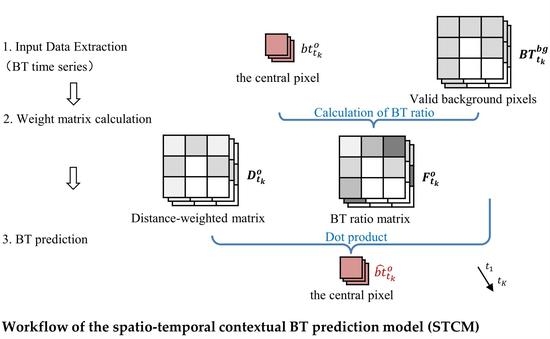
3.2. Spatio-Temporal Contextual Model (STCM)

The STCM proposed in this paper includes three steps: input data extraction, weight matrix calculation, and BT prediction. The accuracy of STCM was evaluated by comparing the predicted value with observed value. STCM workflow is illustrated in Figure 2.

3.2.1. Input Data Extraction

The input data of the BT prediction model in STCM includes the BT time series data of the central pixels and their background pixels. We defined the times series pixels at the location of potential fire pixels on the fire date, 22 October 2007, as the central pixels. First, cloud detection was performed using a method based on that used in the production of the International Geosphere Biosphere Program (IGBP) AVHRR-derived Global Fire Product. Daytime cloud pixels were masked by the combination of the fixed threshold of the reflectance in bands 1 and 2 and the BT in band 32 [33]. Water pixels were then identified using the 1-km land/sea mask contained in the MOD03 data. The daytime potential fire pixels were identified by the fixed threshold of the reflectance in band 2 and the BT in bands 22 and band 31, and the absolute threshold test in band 22 was used to exclude absolute fire pixels. Valid neighboring pixels were identified by the method of that used in the contextual algorithm. Then, time series BT of central pixels and their background pixels were extracted [10].

3.2.2. Weight Matrix Calculation

A potential fire pixel was randomly selected to study the distribution of correlation coefficients between it and its background pixels of time series data. In Figure 3 and Figure 4, 441 group data in a window (21 × 21) with a length of 61 images from 22 August to 21 October 2009, were used to perform correlation analysis. The proportion of pixels with correlation coefficients ranging from 0.7 to 1 was 99.27% (p < 0.05), which indicated that it is necessary to take the relationship between the central pixels and their background pixels into account to predict the BT of the central pixels. Additionally, the closer the distance between the background pixel and the central pixel, the higher the correlation coefficient was, which indicated that the distance between the background pixel and the central pixel needs to be considered as the window grows to obtain a more accurate BT prediction result. Therefore, BT ratio matrix and distance-weighted matrix need to be calculated to quantify the contribution of the background pixel to the BT prediction of the potential fire pixel (i.e., the central pixel).

BT Ratio Matrix Construction

The fixed background window size (21 × 21) used in TCM may lead to data redundancy. In this paper, we used a dynamic window to construct the BT ratio matrix, and the window size of the background pixels increased from 3 × 3 to 21 × 21 until at least 25% of the valid background pixels were within the window. The BT ratio between the central pixel (o) and its valid background pixels n at time t k will be replaced by the value of the previous moment ( t k 1 ) if the background pixels n at time t k are defined as non-valid background pixels. In other words, the correlation between the central pixel and one of its background pixels is abandoned if the background pixel has invalid value. In addition, the determination of optimal weighted parameter ( ρ ) and the number of images (k) in BT ratio matrix is discussed in Section 5.2. We chose 𝜌 = 0.25 and k = 28 in this paper.
F t k n = F t k 1 n

Distance-Weighted Matrix Construction

Different background pixels are assigned different weights based on the distance weighted interpolation (IDW) method [34,35] to improve the accuracy of the BT prediction model. Weighted function is shown in Equation (9):
w i = h i p i = 1 N h i p
where w i is the distance weight of the background pixel I and p is a positive real number, which used to control the impact of known pixels on the unknown pixels. The p value between [0.5, 3] can obtain reasonable results, and the default value is 2. The h i is the distance between the background pixel i and the central pixel, respectively. The distance between the central pixel and its background pixels was determined by the following rules (Table 2).

3.2.3. BT Prediction

The BT of central pixel (o) at time t k can be predicted by Equation (10):
b t ^ t k 0 = D t k o :   F t k o : BT t k b g
where b t ^ t k 0 is the predicted BT of the central pixel o at time t k and calculated by inner-product computation from distance weighted matrix D t k o , BT ratio matrix F t k , o and the BT matrix of the valid background pixels BT t k b g .

3.3. Statistical Analysis

This paper used two metrics to measure the similarity of two time series data and two indicators to evaluate the performance of the BT prediction model, including:

Pearson Correlation Coefficient (PCC)

PCC, also referred to as Pearson’s r, is a measure of the linear correlation between the time series data of the BT of central pixels and their background pixels. It has a value between [−1, 1], where 1 is total positive linear correlation, 0 is no linear correlation, and −1 is total negative linear correlation. The r with absolute value between (0.8, 1.0] is extremely related, (0.6, 0.8] is strongly related, (0.4, 0.6] is moderately related, (0.2, 0.4] is weakly related, and (0.0, 0.2] is very weak or has no correlation.
a.
Kendall’s Coefficient (τ) of Rank Correlation
The τ was used to quantify the agreement between the BT of two images at different times, which varied from −1 to 1. The τ = 1 indicates that the two images exhibit a preponderance of concordant pairs and a strong positive relationship; τ = −1 indicates that the two images show a strong negative relationship. The τ can be calculated as follows:
τ = C D n n 1 / 2
where C is the number of concordant pairs with the same sign (positive or negative), D is the number of discordant pairs, and n is the number of the shared valid pixels of two images [36].
b.
Root–Mean–Square Error (RMSE)
RMSE measures the differences between the predicted BT value and the observed BT value of the central pixels [37].
R M S E = i = 1 N b t i o b t ^ i o 2 N
where b t i o , b t ^ i o are the observed BT value and predicted BT value of the central pixel i, respectively. N is the number of the potential fire pixels. The smaller the RMSE, the higher the accuracy of the model is.
c.
Bias
We calculated the bias between the observed BT and predicted BT of the central pixels. The smaller the absolute value, the smaller the difference between the two values is.

4. Results

Figure 5 shows the potential fire pixels extracted from the image on 22 October 2007: A total of 224 potential fire pixels were identified. The potential fire pixels were mainly distributed in the left-middle part and the left-lower part of the study area.
The BT threshold of bands 22 and 31 and the difference of BT between the two bands were used to identify relative fire pixels in the contextual algorithm. Therefore, we predicted the daily BT of 224 central pixels from August 22 to 21 October 2007 with a total of 61 frames, including the BT of bands 22 and 31 and the difference between the two bands. The root-mean-square error (RMSE) and bias were used to measure the accuracy of the different BT prediction model.

4.1. RMSE of the Predicted BT

We first compared the RMSEs of predicted BT calculated by the three methods for all potential fire pixels (Figure 6). The result showed that the RMSE of STCM was smaller than that of TCM and CM for three physical quantities. Although the minimum RMSE of CM was the smallest, STCM obtained the smallest maximum, quartile, median, and the range of RMSE among the three methods. The lower quartile, median, and the range of RMSE evidenced the superiority of TCM over CM in band 22; however, this superiority was not obvious in band 31 or the difference of the two bands. Overall, STCM significantly improved the BT prediction accuracy and exhibited a more robust result compared with CM and TCM, and the accuracy of TCM in some bands was lower than that of CM.
In order to quantify the superiority of STCM over TCM and CM, Table 3 shows the mean, maximum, minimum, and standard deviation of the RMSE for the three physical quantities calculated by STCM, TCM, and CM, respectively. It can be seen that the average RMSE of STCM was 1.43 of band 22, 1.49 of band 31, and 0.94 of the difference between the two bands, and was 12.54% lower than that of CM and 9.12% lower than that of TCM. The maximum RMSE of STCM was 12.90% and 10.52% lower than that of CM and TCM, respectively. The minimum value was 25.61% higher and 6.07% lower than that of CM and TCM, respectively. The standard deviation was 12.04% and 15.57% lower, respectively. The CM can obtain the smallest minimum RMSE, while other statistical values of RMSE of CM were relatively larger than STCM. The statistics of RMSE of STCM were both smaller than that of TCM, and the standard deviation of TCM was higher than that of CM, which shows that the STCM can get highest accuracy, followed by TCM and CM, while the accuracy of the TCM fluctuated greatly.

4.2. Bias Analysis

Figure 7 displays the normal distribution fitting results of the bias between the observed and predicted values of 224 potential fire pixels. It can be seen that the bias of three physical quantities in different models had similar laws: The range of bias for band 22 was the largest, followed by band 31 and the two-band difference. The bias of the three physical quantities in CM was obviously right deviation (μ = 0.231 for band 22, 0.132 for band 31, and 0.099 for the difference of the two bands), indicating that the prediction value of the CM model was overestimated, while the mean biases of TCM and STCM were closer to 0 and the STCM exhibited better results. The standard deviation of the bias of STCM was the smallest (0.101 for band 22, 0.091 for band 31, and 0.052 for the difference of the two bands) and the fitted curve was the steepest among the three methods, indicating that the distribution of bias of STCM was most concentrated in the vicinity of the mean, followed by TCM, while the distribution of CM was dispersed. In addition, the range of bias of STCM was smallest (−0.36~0.25 of band 22, −0.33~0.20 of band 31, and −0.14~0.14 of the difference of the two bands) and was 15.3% and 88.7% lower than that of TCM and CM, respectively. These differences indicated the superiority of TCM over CM and the superiority of STCM over both TCM and CM.

5. Discussion

5.1. The Influence of Parameter Selection on the Accuracy of STCM

The time-weighted parameter ( ρ ) and the number of images (k) are the two most important parameters in STCM. The spatial variability of thermal landscapes was assumed to be stable in a short period; therefore, the relationship of BT between the central pixel and its surrounding pixels will not change within this period. However, this relationship may vary from one period to another period because the BT within a certain spatial range exhibits differentiated seasonality among different land covers or under complex environmental conditions [38]. Therefore, it is necessary to understand the dynamics of thermal landscapes and to identify the proper period for predicting BT. In this paper, we used a set of weighted parameters ( ρ ), ranging from 0.05 to 1.00 with a step of 0.05, and different number of images (k), ranging from 5 to 60 with a step of 5, to explore the effect of the ρ and k on the accuracy of STCM. The change in RMSE of STCM with different ρ and k (Figure 8) demonstrated that (1) as the number of imageries increased, the RMSE of STCM had a significant decrease. More historical images can result in stable and higher accuracy. It implied that the correlation between the central pixel and its background pixels calculated by long-term data is more robust than that calculated by instantaneous data. (2) The smaller the value of ρ , the more images were required for RMSE to reach a steady state. For example, the RMSE of STCM with ρ = 0.05 was still showing a downward trend in the use of 60 images, while the RMSE of STCM with ρ > 0.75 was stable with the increase of the images. (3) The accuracy of three physical quantities (i.e., BT of bands 22 and 31 and the BT difference of the two bands) had similar performance. The RMSE of the difference between the two bands exhibited a characteristic of first rise and then drop with the increase of the images. Overall, it is necessary to include more historical images to achieve higher prediction accuracy.

5.2. Application of STCM

Although STCM was designed for BT prediction, it can also be applied to the prediction of other environmental variables with high spatial and temporal autocorrelation, such as surface temperature, vegetation index, evapotranspiration, etc. The most important process of STCM is the determination of parameters. The determination of the time-weighted parameter (ρ) and the number of images (k) for BT prediction was elaborated as follows to provide guidelines for the prediction of other environmental variables.
When performing BT prediction, we employed two indicators to determine the optimal parameters in STCM. Bechtel proved that historical information is meaningful for predicting the mean and amplitude of the annual cycles in surface temperature: 35 historical images included in the prediction resulted in an accuracy of approximately 1 k [39]. To determine the optimal number of historical images (k), we first explored the change in BT agreement between two images with different time intervals (from one day to 60 days) by using Kendall’s coefficient of rank correlation τ (Figure 9). Of the images with time interval less than 30 days, 44.83% had τ values greater than 0.7, while only 6.67% of the images with time interval greater than 30 days had τ values greater than 0.7. The two images with time intervals of less than 30 days displayed a strong and stable agreement. It demonstrated that the thermal landscape heterogeneity will not change over about 30 days.
Secondly, we ignored the contribution of the image with weight coefficient ( ρ · 1 ρ k ) of less than 1 × 10 5 . The minimum number of images required for STCM can then be calculated by setting the time-weighted parameter (ρ). As illustrated in Figure 10, the smaller the value of ρ , the smaller the minimum number of images required. In order to provide sufficient historical images while preventing substantial changes in climate or surface conditions [22], we chose ρ = 0.25 and k = 28 to ensemble long-term images to predict BT.

5.3. Advantages and Limitations

The thermal infrared landscape is affected by environmental factors, such as topography, latitude, vegetation types, etc., [38,40,41]. The BT relation matrix (i.e., BT ratio of the central pixel and its surrounding pixels) used in STCM enables it to describe the heterogeneity of BT caused by these environmental factors. Moreover, the participation of historical images makes the BT relation matrix more stable, which makes the STCM robust and less affected by disturbing factors such as cloud and wind. Additionally, STCM has the potential to improve fire detection accuracy. After obtaining the predicted BT of the potential pixels, the predicted BT and the true BT were compared to identify the fire pixel in CM and TCM. If the difference between the predicted value and true value exceeded the given threshold, this potential pixel was considered as the fire point. Therefore, the accuracy of the BT prediction is crucial for improving fire detection accuracy. Compared with CM and TCM, STCM gave the best performance for BT prediction for potential fire pixels, and the BT of the potential pixels calculated by STCM using stable time series data is more likely to characterize the situation where no fire occurred when a fire occurs.
However, it should be noted that the STCM also contains a few limitations. The model has higher requirements for data quality and continuity. In this paper, the number of images were set as 28 and the time-weighted parameter was set as 0.25 to get higher prediction accuracy of BT. However, due to the effects of clouds, snow, pixel saturation issues, etc., the proportion of valid background pixels within a given window that were used to predict the BT of central pixels was often less than 25% [42], which will significantly reduce the number of usable images. Therefore, STCM is not applicable in high cloud or snow-covered areas. Additionally, the same problem will be found in the later period of the fire. As the fire spreads, the number of background pixels around the potential fire point that can be used to predict BT under normal situation will decrease significantly. If this number is less than 25% of all neighborhood pixels, the STCM will achieve poor prediction performance. So, the STCM is limited to the early period of the fire or small fires. Additionally, the accompanying data inspection and processing are time consuming. Despite these limitations of STCM, it is acceptable and feasible in actual operation.
It is worth noting that further studies should use the BT prediction results to detect fire pixels and the influence of the error in BT prediction on the accuracy of fire detection. Additionally, although STCM exhibited robust performance in BT prediction in San Diego, its generality is still unclear in terms of the study area. It is necessary to apply the STCM to more regions in different climatic zones or with different land characteristics in further study.

6. Conclusions

To improve the accuracy of the BT prediction, this paper proposed a spatio-temporal BT prediction model (STCM), which introduced a distance-weighted matrix to correct the BT correlation between the central pixel and its surrounding pixels in the time-weighted spatial context BT prediction model (TCM). Additionally, a dynamic window that used to calculate the BT correlation matrix was employed to improve the efficiency of the prediction process. The proposed method was applied to BT prediction of 224 central pixels (i.e., potential fire pixels) on 21 October 2007 in San Diego based on historical MODIS BT time series and was compared with the CM and TCM. The result demonstrated that STCM can effectively improve the accuracy of BT prediction of the central pixels. The mean RMSE of STCM was 12.54% lower than that of CM and 9.12% lower than that of TCM. The bias of STCM was closer to zero and the range of bias was 88.7% and 15.3% lower than that of CM and TCM, respectively. In addition, the method of determining the optimal parameters (e.g., time-weighted parameter and the number of historical images) was given to provide a reference for the application of STCM and other environmental variables.

Author Contributions

J.L. had the original idea for the study and wrote the original manuscript. A.G. supervised the research and edited the manuscript. Y.C. aided with the discussion and the manuscript revision. All authors have read and agreed to the published version of the manuscript.

Funding

This research was jointly supported by the National Key Research and Development Program of China (Grant No. 2017YFB0504102, No. 2017YFC1502402, and Nos. 2019YFE01277002 and 2017YFC1502704-01) and the National Natural Science Foundation of China (41671412).

Institutional Review Board Statement

Not applicable.

Informed Consent Statement

Not applicable.

Data Availability Statement

Not applicable.

Conflicts of Interest

The authors declare no conflict of interest.

References

  1. Wright, R.; Flynn, L.; Garbeil, H.; Harris, A.; Pilger, E. Automated volcanic eruption detection using MODIS. Remote Sens. Environ. 2002, 82, 135–155. [Google Scholar] [CrossRef] [Green Version]
  2. Ardakani, A.S.; Zoej, M.J.V.; Mohammadzadeh, A.; Mansourian, A. Spatial and temporal analysis of fires detected by MODIS data in northern Iran from 2001 to 2008. IEEE J. Sel. Topics Appl. Earth Observ. Remote Sens. 2010, 4, 216–225. [Google Scholar] [CrossRef]
  3. Mazzeo, G.; Marchese, F.; Filizzola, C.; Pergola, N.; Tramutoli, V. A Multi-temporal Robust Satellite Technique (RST) for forest fire detection. In Proceedings of the 2007 International Workshop on the Analysis of Multi-temporal Remote Sensing Images, Leuven, Belgium, 18–20 July 2007; pp. 1–6. [Google Scholar]
  4. Ya’acob, N.; Najib, M.S.M.; Tajudin, N.; Yusof, A.L.; Kassim, M. Image processing based forest fire detection using infrared camera. J. Phys. Conf. Ser. 2021, 1768, 012014. [Google Scholar] [CrossRef]
  5. Piñol, J.; Terradas, J.; Lloret, F. Climate warming, wildfire hazard, and wildfire occurrence in coastal eastern Spain. Clim. Chang. 1998, 38, 345–357. [Google Scholar] [CrossRef]
  6. Pierce, J.; Meyer, G. Long-term fire history from alluvial fan sediments: The role of drought and climate variability, and implications for management of Rocky Mountain forests. Int. J. Wildland Fire 2008, 17, 84–95. [Google Scholar] [CrossRef] [Green Version]
  7. Running, S.W. Is global warming causing more, larger wildfires? Science 2006, 313, 927–928. [Google Scholar] [CrossRef] [Green Version]
  8. Wang, S.-D.; Miao, L.; Peng, G.-X. An improved algorithm for forest fire detection using HJ data. Procedia Environ. Sci. 2012, 13, 140–150. [Google Scholar] [CrossRef] [Green Version]
  9. Tomlinson, C.J.; Chapman, L.; Thornes, J.E.; Baker, C. Remote sensing land surface temperature for meteorology and climatology: A review. Meteorol. Appl. 2011, 18, 296–306. [Google Scholar] [CrossRef] [Green Version]
  10. Giglio, L.; Descloitres, J.; Justice, C.O.; Kaufman, Y.J. An enhanced contextual fire detection algorithm for MODIS. Remote Sens. Environ. 2003, 87, 273–282. [Google Scholar] [CrossRef]
  11. Giglio, L.; Loboda, T.; Roy, D.P.; Quayle, B.; Justice, C.O. An active-fire based burned area mapping algorithm for the MODIS sensor. Remote Sens. Environ. 2009, 113, 408–420. [Google Scholar] [CrossRef]
  12. Van der Werf, G.R.; Randerson, J.T.; Giglio, L.; Collatz, G.; Mu, M.; Kasibhatla, P.S.; Morton, D.C.; DeFries, R.; Jin, Y.v.; van Leeuwen, T.T. Global fire emissions and the contribution of deforestation, savanna, forest, agricultural, and peat fires (1997–2009). Atmos. Chem. Phys. 2010, 10, 11707–11735. [Google Scholar] [CrossRef] [Green Version]
  13. Roy, D.P.; Frost, P.; Justice, C.; Landmann, T.; Le Roux, J.; Gumbo, K.; Makungwa, S.; Dunham, K.; Du Toit, R.; Mhwandagara, K. The Southern Africa Fire Network (SAFNet) regional burned-area product-validation protocol. Int. J. Remote Sens. 2005, 26, 4265–4292. [Google Scholar] [CrossRef]
  14. Mouillot, F.; Schultz, M.G.; Yue, C.; Cadule, P.; Tansey, K.; Ciais, P.; Chuvieco, E. Ten years of global burned area products from spaceborne remote sensing—A review: Analysis of user needs and recommendations for future developments. Int. J. Appl. Earth Obs. Geoinf. 2014, 26, 64–79. [Google Scholar] [CrossRef] [Green Version]
  15. Boschetti, L.; Roy, D.P.; Justice, C.O.; Humber, M.L. MODIS–Landsat fusion for large area 30 m burned area mapping. Remote Sens. Environ. 2015, 161, 27–42. [Google Scholar] [CrossRef]
  16. Fu, Y.; Li, R.; Wang, X.; Bergeron, Y.; Valeria, O.; Chavardès, R.D.; Wang, Y.; Hu, J. Fire detection and fire radiative power in forests and low-biomass lands in Northeast Asia: MODIS versus VIIRS fire products. Remote Sens. 2020, 12, 2870. [Google Scholar] [CrossRef]
  17. Flasse, S.; Ceccato, P. A contextual algorithm for AVHRR fire detection. Int. J. Remote Sens. 1996, 17, 419–424. [Google Scholar] [CrossRef]
  18. Giglio, L.; Schroeder, W.; Justice, C.O. The collection 6 MODIS active fire detection algorithm and fire products. Remote Sens. Environ. 2016, 178, 31–41. [Google Scholar] [CrossRef] [PubMed] [Green Version]
  19. Amraoui, M.; DaCamara, C.; Pereira, J. Detection and monitoring of African vegetation fires using MSG-SEVIRI imagery. Remote Sens. Environ. 2010, 114, 1038–1052. [Google Scholar] [CrossRef]
  20. Csiszar, I.; Schroeder, W.; Giglio, L.; Ellicott, E.; Vadrevu, K.P.; Justice, C.O.; Wind, B. Active fires from the Suomi NPP Visible Infrared Imaging Radiometer Suite: Product status and first evaluation results. J. Geophys. Res. Atmos. 2014, 119, 803–816. [Google Scholar] [CrossRef]
  21. Wooster, M.J.; Xu, W.; Nightingale, T. Sentinel-3 SLSTR active fire detection and FRP product: Pre-launch algorithm development and performance evaluation using MODIS and ASTER datasets. Remote Sens. Environ. 2012, 120, 236–254. [Google Scholar] [CrossRef]
  22. Bechtel, B. Robustness of annual cycle parameters to characterize the urban thermal landscapes. IEEE Geosci. Remote. Sens. Lett. 2012, 9, 876–880. [Google Scholar] [CrossRef]
  23. Laneve, G.; Castronuovo, M.M.; Cadau, E.G. Continuous monitoring of forest fires in the Mediterranean area using MSG. IEEE Trans. Geosci. Remote Sens. 2006, 44, 2761–2768. [Google Scholar] [CrossRef]
  24. Roberts, G.; Wooster, M. Development of a multi-temporal Kalman filter approach to geostationary active fire detection & fire radiative power (FRP) estimation. Remote Sens. Environ. 2014, 152, 392–412. [Google Scholar]
  25. Su, Y.R. MODIS forest detection method using mixed pixel decomposition. Bachelor’s Thesis, Beijing Normal University, Beijing, China, 2015. [Google Scholar]
  26. Pavlidou, E.; van der Meijde, M.; van der Werff, H.; Hecker, C. Finding a needle by removing the haystack: A spatio-temporal normalization method for geophysical data. Comput Geosci. 2016, 90, 78–86. [Google Scholar] [CrossRef]
  27. Lin, L.; Meng, Y.; Yue, A.; Yuan, Y.; Liu, X.; Chen, J.; Zhang, M.; Chen, J. A spatio-temporal model for forest fire detection using HJ-IRS satellite data. Remote Sens. 2016, 8, 403. [Google Scholar] [CrossRef] [Green Version]
  28. Kottek, M.; Grieser, J.; Beck, C.; Rudolf, B.; Rubel, F. World map of the Köppen-Geiger climate classification updated. Meteorol. Z. 2006, 15, 259–263. [Google Scholar] [CrossRef]
  29. Pugnaire, F.; Valladares, F. Functional Plant Ecology; CRC Press: Boca Raton, FL, USA, 2007. [Google Scholar]
  30. Wan, Z. MODIS Level 1B Algorithm Theoretical Basis Document. Institute for Computational Earth System Science, University of California: Santa Barbara, CA, USA, 1999. [Google Scholar]
  31. Sabins, F.F. Remote Sensing: Principles and Applications; Waveland Press: Long Grove, IL, USA, 2007. [Google Scholar]
  32. Qin, Z.; Gao, M.; Qin, X. Methodology to inverse land surface temperature from MODIS data for agricultural drought monitoring in China. J. Nat. Disaster Sci. 2005, 14, 64. [Google Scholar]
  33. Stroppiana, D.; Pinnock, S.; Gregoire, J.-M. The global fire product: Daily fire occurrence from April 1992 to December 1993 derived from NOAA AVHRR data. Int. J. Remote Sens. 2000, 21, 1279–1288. [Google Scholar] [CrossRef]
  34. Zhan, H.; Xie, W.; Sun, H.; Huang, H. Using ENVI-met to simulate 3D temperature distribution in vegetated scenes. J. Beijing For. Univ. 2014, 36, 64–74. [Google Scholar]
  35. Zhang, F.C.; Sun, X.G. Application of inverse distance weighted interpolation method in finite temperature point temperature field. Appl. Mech. Mater 2014, 599, 1268–1271. [Google Scholar]
  36. Kendall, M.G.; Kendall, S.F.; Smith, B.B. The distribution of Spearman’s coefficient of rank correlation in a universe in which all rankings occur an equal number of times. Biometrika 1939, 30, 251–273. [Google Scholar]
  37. Hyndman, R.J.; Koehler, A.B. Another look at measures of forecast accuracy. Int. J. Forecast. 2006, 22, 679–688. [Google Scholar] [CrossRef] [Green Version]
  38. Weng, Q.; Fu, P.; Gao, F. Generating daily land surface temperature at Landsat resolution by fusing Landsat and MODIS data. Remote Sens. Environ. 2014, 145, 55–67. [Google Scholar] [CrossRef]
  39. Bechtel, B.; Daneke, C. Classification of local climate zones based on multiple earth observation data. IEEE J. Sel. Topics Appl. Earth Observ. 2012, 5, 1191–1202. [Google Scholar] [CrossRef]
  40. Weng, Q.; Lu, D.; Schubring, J. Estimation of land surface temperature–vegetation abundance relationship for urban heat island studies. Remote Sens. Environ. 2004, 89, 467–483. [Google Scholar] [CrossRef]
  41. Weng, Q.; Liu, H.; Liang, B.; Lu, D. The spatial variations of urban land surface temperatures: Pertinent factors, zoning effect, and seasonal variability. IEEE J. Sel. Topics Appl. Earth Observ. 2008, 1, 154–166. [Google Scholar] [CrossRef]
  42. Lemmetyinen, J.; Derksen, C.; Pulliainen, J.; Strapp, W.; Toose, P.; Walker, A.; Tauriainen, S.; Pihlflyckt, J.; Karna, J.-P.; Hallikainen, M.T. A comparison of airborne microwave brightness temperatures and snowpack properties across the boreal forests of Finland and Western Canada. IEEE Trans. Geosci. Remote Sens. 2009, 47, 965–978. [Google Scholar] [CrossRef]
Figure 1. The location of the study area. The forest land of the study area (a) and the MODIS image on 22 October 2007 with the false-color composite imagery from bands 20, 21, and 31. The purple area in the figure was the anomaly area with high temperature (b).
Remotesensing 13 02900 g001
Figure 2. Workflow of the spatio-temporal contextual BT prediction model (STCM).
Remotesensing 13 02900 g002
Figure 3. Correlation coefficients between a central pixel and its background pixels of time series data. The proportion of pixels with correlation coefficients ranging from 0.7 to 1 was 99.27% (p < 0.05).
Remotesensing 13 02900 g003
Figure 4. The frequency distribution of the correlation coefficients between the central pixel and its background pixels of time series data.
Remotesensing 13 02900 g004
Figure 5. The distribution of the potential fire pixels.
Remotesensing 13 02900 g005
Figure 6. The boxplot of RMSE result of the BT prediction by the STCM, TCM, and CM for band 22 (a), band 31 (b), and the difference of the two bands (c). In each box, the central red mark is the median, the edges of the box are the 25th and 75th percentiles, the whiskers extend to the most extreme data points not considered outliers, and outliers are plotted individually if they are larger than q3 + 1.5(q3–q1) or smaller than q1–1.5(q3–q1), where q1 and q3 are the 25th and 75th percentiles, respectively.
Remotesensing 13 02900 g006
Figure 7. The normal distribution of the biases of the STCM (ac), TCM (df), and CM (gi) in band 22, band 31, and the difference of the two bands. The μ is an estimate of the mean and σ is an estimate of the standard deviation of the normal distribution, given the bias data.
Remotesensing 13 02900 g007
Figure 8. The change of RMSE in STCM for band 22 (a), band 31 (b), and the difference of the two bands (c) of different time-weighted parameter ( ρ ) and number of images (k).
Remotesensing 13 02900 g008
Figure 9. The distribution of Kendall’s coefficient of rank correlation τ of BT between two images with time different intervals from one to 60 days. The τ varies from –1 to 1. The τ = 1 indicates that the BT of two images with a preponderance of concordant pairs showed a strong positive relationship; τ = –1 indicates that the BT of two images showed a strong negative relationship.
Remotesensing 13 02900 g009
Figure 10. The minimum number of the images required for STCM with different time-weighted parameter ( ρ ).
Remotesensing 13 02900 g010
Table 1. Band features and its application of MOD02 data.
Band (Central Wavelength/μm)Physical QuantityApplication
1 (0.65) ρ 1 reflectanceCloud masking
2 (0.86) ρ 2 reflectanceCloud masking
7 (2.13) ρ 7 reflectanceCloud masking
22 (4.0) B T 22 BTBT prediction
31 (11.0) B T 31 BTBT prediction, Cloud masking
32 (12.0) B T 32 BTCloud masking
Table 2. The distance rule between the central pixel and its background pixels with window size of 3 × 3.
Remotesensing 13 02900 i001
Table 3. The statistical values of RMSE for STCM, TCM, and CM for bands 22 and 31 and the difference of the two bands (D).
ModelMeanMaximumMinimumStandard Deviation
Band2231D2231D2231D2231D
CM1.741.711.013.854.392.270.870.720.240.550.900.63
TCM1.571.651.033.674.242.271.020.800.410.590.950.63
STCM1.431.490.943.203.802.080.910.760.400.470.820.55
Publisher’s Note: MDPI stays neutral with regard to jurisdictional claims in published maps and institutional affiliations.

