Fast Complex-Valued CNN for Radar Jamming Signal Recognition

Abstract

Jamming is a big threat to the survival of a radar system. Therefore, the recognition of radar jamming signal type is a part of radar countermeasure. Recently, convolutional neural networks (CNNs) have shown their effectiveness in radar signal processing, including jamming signal recognition. However, most of existing CNN methods do not regard radar jamming as a complex value signal. In this study, a complex-valued CNN (CV-CNN) is investigated to fully explore the inherent characteristics of a radar jamming signal, and we find that we can obtain better recognition accuracy using this method compared with a real-valued CNN (RV-CNN). CV-CNNs contain more parameters, which need more inference time. To reduce the parameter redundancy and speed up the recognition time, a fast CV-CNN (F-CV-CNN), which is based on pruning, is proposed for radar jamming signal fast recognition. The experimental results show that the CV-CNN and F-CV-CNN methods obtain good recognition performance in terms of accuracy and speed. The proposed methods open a new window for future research, which shows a huge potential of CV-CNN-based methods for radar signal processing.

1. Introduction

Due to the powerful capability to detect, recognize, and track targets under the conditions of all weather, radar is widely used in many weapon systems, and it has become an indispensable electronic equipment in military [1]. With the continuous development of radar jamming technology, many radar jamming technologies have been developed to attack radar systems in order to reduce their target detection, recognition, and tracking capabilities [2]. In addition to various radar jamming methods, more and more electromagnetic signal use in the battlefield environment also seriously affects the effectiveness of the radar system. Radar anti-jamming technology is used for protecting the radar from jamming [3]. As an important prerequisite for effective anti-jamming measures, radar jamming signal recognition has received more and more attention.

Recently, many recognition approaches of radar jamming signals have been proposed, including likelihood-based methods [4,5,6] and feature-based methods [7,8,9,10,11,12,13]. Based on the prior information, the likelihood-based methods identify the type of jamming signal by matching the likelihood function of the jamming signal with some determined thresholds. For instance, based on the adaptive coherent estimator and the generalized likelihood ratio test (GLRT), Greco et al. [4] proposed a deception jamming recognition method. Moreover, in [5], an adaptive detection algorithm based on the GLRT implementation of a generalized Neyman–Pearson rule was proposed to discriminate radar targets and electronic countermeasure (ECM) signals. In addition, Zhao et al. [6] utilized the conventional linear model to discriminate the target and radar jamming signal. Unfortunately, neither the necessary prior information nor the appropriate threshold can be guaranteed in reality, which limits the application of likelihood-based methods for radar jamming signal recognition.

Compared with the signal in the original domain, the extracted features in the transformation domain are usually more separable. Therefore, some jamming signal recognition methods based on feature extraction were proposed. The feature-based method consists of feature extraction and classifier selection. Many researchers extract distinguishing features from jamming signal based on multi-domains, including the time domain [7], frequency domain [8], time–frequency domain [9], and so on. For example, using the product spectrum matrix (SPM), Tian et al. [10] proposed a deception jamming recognition method. Moreover, in [11], support vector machine (SVM) was selected as a classifier to recognize chaff jamming. In [12], based on the AdaBoost.M1 algorithm, a radar jamming recognition algorithm that selected SVM as the component classifiers was proposed. In addition, based on different classifiers (i.e., decision tree, neural network, and support vector machine), Meng et al. [13] extracted five features of jamming signals, including three time-domain features and two frequency-domain features, which could increase the robustness of the recognition system. Nevertheless, the aforementioned methods require a lot of manpower, and high time costs still remain for these approaches based on feature extraction.

Recently, CNN, which is one of the popular deep learning models, has achieved great performance in many fields, including image, text, and speech processing [14]. Due to the uniqueness of the network structure of CNN (e.g., local connections and shared weights), CNN-based methods can automatically extract the invariant and discriminant features of data [15]. Moreover, a growing number of CNN-based methods have been proposed in the field of jamming recognition [16,17,18,19]. In [16], a well-designed CNN was utilized to recognize active jamming, and the results indicated that CNNs had the power and ability to distinguish active jamming. In addition, in [17], a CNN-based method was proposed for the recognition of radar jamming, which could recognize nine typical radar jamming signal. By integrating residual block and asymmetric convolution block, Qu et al. [18] proposed a jamming recognition network, which could better extract the features of jamming signals. Moreover, based on the CNN, Wu et al. [19] proposed an automatic radar jamming signal recognition method, which could recognize five kinds of radar jamming signal. Andriyanov et al. used CNN in radar image processing, and they analyzed the construction process of CNN in detail [20]. The recognition rate and recall rate of radar images could reach more than 90%, which illustrated the effectiveness of CNN in processing radar data. Recently, Shao et al. designed a 1D-CNN for radar jamming signal recognition that can identify 12 types of radar jamming with a recognition accuracy of up to 97% [21], which also illustrated the effectiveness of the CNN-based method in processing radar jamming signals.

Radar signals, including radar jamming signals, are naturally complex-valued (CV) based data, including real part and imaginary part. CV data contain more information than RV data, i.e., amplitude $r$ and phase $\theta$. When processing the CV signal, neither the phase nor amplitude information should be ignored.

In order to make full use of the phase and amplitude information of radar jamming signals, a bispectrum analysis was used to keep the phase and amplitude information of the CV signal [22]. Moreover, some researchers have proposed several methods for CV jamming signal recognition [23,24]. For example, based on the amplitude fluctuation, high-order cumulant, and bispectrum, Li et at. studied the feature extraction to analyze and compare the features of deception jamming and target echo [23]. In [24], an algorithm that utilized the bispectrum transformation to extract the amplitude and phase features was proposed to identify deception jamming.

However, most of the existing RV-CNN-based jamming recognition methods mentioned above converted the CV jamming signal into RV and would then input them into RV-CNN for jamming recognition. Since the input and model parameters of the RV-CNN-based methods are RV, they have insufficient significance for phase and amplitude information and are more suitable for processing RV data. For this reason, the loss of phase and amplitude information caused by RV-CNN-based methods is unavoidable, and the problem that RV-CNN cannot fully extract the features of CV data still exists.

Apparently, it is better to extract the CV jamming signal in a complex domain, which can make better use of the unique information of the CV signal, such as phase and amplitude. Therefore, in our work, a radar jamming signal recognition approach based on CV-CNN is proposed. The proposed CV-CNN consists of multiple CV layers, including a CV input layer, several alternations of CV convolutional layers, CV pooling layers, and so on. By extending the entire network parameters to a complex domain, the proposed CV-CNN is able to extract CV features from the jamming signal more efficiently than the aforementioned RV-CNN.

Although a CV-CNN can deal with the CV jamming signal perfectly, due to the complex expansion of the entire model, the CV-CNN still suffers from high computational complexity. Unfortunately, jamming signal recognition tasks have strict requirements for real-time performance, making it difficult to deploy a CV-CNN in the resource-constrained battlefield environments. For deep learning model compression, model pruning [25] is a quite effective method by eliminating redundant parameters. Most model pruning methods [26,27,28] pruned the less important weight of the model in the filter. Therefore, in our work, motivated by filter pruning, a simple yet effective F-CV-CNN algorithm is proposed for accelerating the CV-CNN.

The main contributions of this study are listed as followed:

• To address the issue that the existing RV-CNN cannot make good use of CV jamming signal, a CV-CNN is proposed to simultaneously extract the features of real and imagery radar signals, which improves the recognition accuracy of a radar jamming signal.
• In addition, in view of the high real-time requirements of radar jamming recognition tasks, the fast CV-CNN algorithm is proposed to accelerate the recognition speed of the CV-CNN.

The rest of this paper is organized as follows. The proposed methodology of the CV-CNN for CV jamming signal recognition is provided in Section 2. The proposed fast CV-CNN algorithm process is then shown in Section 3. The details of the experiment, the experimental results and the analysis of results are presented in Section 4, followed by the conclusion presented in Section 5.

2. Proposed CV-CNN for Radar Jamming Signal Recognition

In this section, to address the problem that existing neural network methods cannot make full use of the CV information of radar jamming signal, a novel CV-CNN is proposed. The proposed CV-CNN extends the network parameters from real number to complex number. It is expected that the CV-CNN efficiently extracts the features from the radar jamming signal compared with the existing RV-CNN.

2.1. RV-CNN-Based Radar Jamming Signal Recognition

In this subsection, well-designed single-path RV-CNN (S-RV-CNN) and dual-path RV-CNN (D-RV-CNN) are utilized to extract the abstract features. The structures of the S-RV-CNN and D-RV-CNN are shown in Figure 1 and Figure 2, respectively.

As shown in Figure 1, the S-RV-CNN only contains one channel, and the input is the RV data after the real and imaginary parts of the CV jamming signal are connected. The S-RV-CNN contains an input layer, along with several alternations of the convolutional layers and pooling layers.

In Figure 2, it can be seen that the D-RV-CNN structure consists of two identical S-RV-CNNs—one for extracting the real features and the other for the imaginary features. In the D-RV-CNN, firstly, the real part and imaginary part of the CV jamming signal are fed as inputs into two identical RV-CNNs for each respective part, and the real part and imaginary part features of the CV jamming signal are extracted. Secondly, the extracted real and imaginary part features of the CV radar jamming signal are concatenated, and then are fed as input to the full connection (FC) layer for feature integration. Finally, the eigenvector is fed as input into the Softmax classifier to obtain the recognition result of the CV radar jamming signal.

The convolutional layer is the unique structure of the CNN; it extracts the features of the jamming signal automatically via multiple convolution kernels with different filter sizes. The convolution operation can be defined as:

$$v_j^l={\displaystyle \sum }_{\mathrm{i}=1}^{\mathrm{M}}{v}_i^{l-1}\ast w_{ij}^l+b_j^l,$$

(1)

where $M$ is the number of input feature maps of jamming signal; matrix $v_i^{l-1}$ denotes the $i$-th feature map of the $\left(l-1\right)$-th layer; the current layer output feature map is $v_j^l$; $\ast$ is the convolution operator; and $w_{ij}^l$ and $b_j^l$ are the connection weight and bias, respectively.

In this study, the max-pooling operation was used to reduce the data dimension. In addition, the rectified linear unit (ReLU) activation function was used to extract the nonlinear features of radar jamming signal [12].

Moreover, in order to accelerate the convergence speed of the network, a batch normalization (BN) layer was introduced in the D-RV-CNN [13], which can be defined as follows:

$$\mathrm{BN}\left(\mathrm{x}\right)=\gamma \frac{{\mathrm{x}}^{\mathrm{i}}-\frac{1}{\mathrm{m}}{{\displaystyle \sum }}_{\mathrm{i}=1}^{\mathrm{m}}{\mathrm{x}}^{\mathrm{i}}}{\sqrt{\frac{1}{\mathrm{m}}{{\displaystyle \sum }}_{\mathrm{i}=1}^{\mathrm{m}}({\mathrm{x}}_{\mathrm{i}}-\frac{1}{\mathrm{m}}{{\displaystyle \sum }}_{\mathrm{i}=1}^{\mathrm{m}}({\mathrm{x}}^{\mathrm{i}}){)}^2+\mathsf{\epsilon }}}+\beta ,$$

(2)

where $\gamma$ and $\beta$ are two learnable parameters for feature reconstruction.

In addition, a dropout [14] and global average pooling (GAP) [15] are introduced in the D-RV-CNN to alleviate the phenomenon of overfitting. As a regularization method, dropout inactivates a neuron with a certain probability during CNN training. By averaging the whole feature map, GAP is able to regularize the structure of the whole network to prevent overfitting.

2.2. CV-CNN-based Radar Jamming Signal Recognition

The proposed CV-CNN framework for radar jamming signal recognition is shown in Figure 3. Similar to the aforementioned D-RV-CNN, the CV-CNN consists of multiple cascaded layers, including a CV input layer, several alternations of CV convolution layers and CV pooling layers, etc.

The input of the CV-CNN is the CV radar jamming signal, and all mathematical operations of CV-CNN are extended under the theory of complex analysis, including forward propagation and backpropagation. Under the analysis of complex theory, CV-CNN is more suitable for processing a CV jamming signal.

The key structure of the CV-CNN is described below. The first part of the CV-CNN is the CV convolution (CConv) layer. CConv is extended from RV convolution, which is more suitable for extracting deep features of a radar jamming signal. Suppose that $a_k^{\left(l-1\right)}\in {ℂ}^{W_{l-1}\times H_{l-1}\times I_{l-1}}$ is the input radar jamming signal feature map in the $l$-th CConv layer, and $ℂ$ represents the complex domain. In the $l$-th CConv layer, the number CConv kernel $w_{ik}^{\left(l\right)}\in {ℂ}^{F_l\times F_l\times I_{l-1}\times I_l}$ is $I$. The output of CV feature map in the $l$-th CConv layer is $z_i^{\left(l\right)}\in {ℂ}^{W_l\times H_l\times I_l}$,

$${\mathrm{z}}_{\mathrm{i}}^{\left(\mathrm{l}\right)}=\mathrm{f}\left(ℛ({\mathrm{V}}_{\mathrm{i}}^{\left(\mathrm{l}\right)})\right)+\mathrm{i}·\left(ℐ({\mathrm{V}}_{\mathrm{i}}^{\left(\mathrm{l}\right)})\right),$$

(3)

where $f\left(·\right)$ represents the non-linear activation function, and $ℛ\left(·\right)$ and $ℐ\left(·\right)$ represent operation of extracting the real part and imaginary part of the CV jamming signal, respectively.

In addition, $V_i^{\left(l\right)}$ represents the result of CConv calculation of the CV feature map $a_k^{\left(l-1\right)}$ and CConv kernel $w_{ik}^{\left(l\right)}$, and the detailed CConv calculation process is shown in Equation (4):

$$\begin{array}{c}{V}_i^{\left(l\right)}={\displaystyle \sum _{\mathrm{k}=1}^{\mathrm{K}}}{w}_{ik}^{\left(l\right)}\ast a_k^{\left(l-1\right)}+b_i^{\left(l\right)}\hfill \\ ={\displaystyle \sum _{k=1}^K}ℛ(w_{ik}^{\left(l\right)})\ast ℛ(a_k^{\left(l-1\right)})-ℐ(w_{ik}^{\left(l\right)})\ast ℐ(a_k^{\left(l-1\right)})+ℛ(b_i^{\left(l\right)}))\hfill \\ +i·{\displaystyle \sum _{k=1}^K}ℛ(w_{ik}^{\left(l\right)})\ast ℐ(a_k^{\left(l-1\right)})-ℐ(w_{ik}^{\left(l\right)})\ast ℛ(a_k^{\left(l-1\right)})+ℐ(b_i^{\left(l\right)})).\hfill \end{array}$$

(4)

The second part of the CV-CNN is the CV activation function. In this work, three CV activate functions are extended from RV ReLU (i.e., modReLU [16], zReLU [17], and cReLU).

The first is the modReLU activation function. By introducing a learnable parameter $b$, modReLU constructs a zero-setting zone with radius $b$. The expression of modReLU is as follows:

$$\mathrm{modReLU}\left(\mathrm{z}\right)=\mathrm{ReLU}\left(\left|\mathrm{z}\right|+b\right){\mathrm{e}}^{\mathrm{i}{\theta }_z}=\{\begin{array}{c}(\left|\mathrm{z}\right|+\mathrm{b})\frac{\mathrm{z}}{\left|\mathrm{z}\right|} if \left(\left|\mathrm{z}\right|+b\right)\ge 0\hfill \\ 0 \mathrm{otherwise}\hfill \end{array},$$

(5)

where z is the input radar jamming feature map, and ${\theta }_z$ is the phase of $z$.

The expression of zReLU is as follows:

$$\mathrm{zReLU}\left(\mathrm{z}\right)=\{\begin{array}{c}z \mathrm{if} 0\le {\theta }_z\le \pi /2\hfill \\ 0 \mathrm{otherwise}\hfill \end{array}.$$

(6)

It can be found from Equation (6) that zReLU retains the CV jamming feature map when the phase is between 0 and $\pi /2$.

According to the phase value, the zReLU performs the ReLU operation on the input CV jamming feature map, while the cReLU performs the ReLU operation on the real and imaginary parts of the input CV jamming feature map separately. The expression of cReLU is as follows:

$$\mathrm{cReLU}\left(\mathrm{z}\right)=\mathrm{ReLU}\left(ℛ\left(\mathrm{z}\right)\right)+\mathrm{i}·\mathrm{ReLU}\left(ℐ\left(\mathrm{z}\right)\right)=\max \left(0,ℛ\left(\mathrm{z}\right)\right)+\mathrm{i}·\max \left(0,ℐ\left(\mathrm{z}\right)\right).$$

(7)

The second part of is CV BN (CBN) layer, which is extended from the real domain to the complex domain. Real-valued BN (RBN) consists essentially of two steps, i.e., standardization, and scaling and shifting. Nevertheless, only transforming and scaling the CV jamming feature map might lead to the deviation of the data distribution. Therefore, it is necessary to perform CBN for the CV jamming signal.

Since a CV jamming signal x consists of real part $ℛ\left(x\right)$ and imaginary part $ℐ\left(x\right)$, we regard $ℛ\left(x\right)$ and $ℐ\left(x\right)$ as two components of $x$. Then the covariance matrix V can be utilized to normalize x to the normalized $\overline{x}$:

$$\overline{\mathrm{x}}={\mathrm{V}}^{-\frac{1}{2}}\left(\mathrm{x}-\mathrm{E}\left[\mathrm{x}\right]\right),$$

(8)

and $V$ can be obtained by:

$$\mathrm{V}=\left(\begin{array}{c}{\mathrm{V}}_{\mathrm{rr}}\\ {\mathrm{V}}_{\mathrm{ir}}\end{array}\begin{array}{c}{\mathrm{V}}_{\mathrm{ri}}\\ {\mathrm{V}}_{\mathrm{ii}}\end{array}\right)=\left(\begin{array}{c}\mathrm{Cov}(ℛ\left(\mathrm{x}\right),ℛ\left(\mathrm{x}\right))\\ \mathrm{Cov}(ℐ\left(\mathrm{x}\right),\mathrm{R}\left(\mathrm{x}\right))\end{array}\begin{array}{c}\mathrm{Cov}(ℛ\left(\mathrm{x}\right),ℐ\left(\mathrm{x}\right))\\ \mathrm{Cov}(ℐ\left(\mathrm{x}\right),ℐ\left(\mathrm{x}\right))\end{array}\right),$$

(9)

where $\mathrm{Cov}(·)$ denotes the covariance function. Similar to RBN, two variables (i.e., scaling parameter $\beta$ and shifting parameter $\gamma$) are introduced to restore the learned features. The CBN operation can be defined as:

$$\mathrm{CBN}(\overline{\mathrm{x}})=\gamma \overline{\mathrm{x}}+\beta ,$$

(10)

where scaling parameters $\beta$ is a CV parameter with two learnable parameters, and $\gamma$ is a $2\times 2$ matrix with three parameters to be learned:

$$\mathsf{\gamma }=\left(\begin{array}{c}{\mathsf{\gamma }}_{\mathrm{rr}}\\ {\mathsf{\gamma }}_{\mathrm{ri}}\end{array}\begin{array}{c}{\mathsf{\gamma }}_{\mathrm{ri}}\\ {\mathsf{\gamma }}_{\mathrm{ii}}\end{array}\right).$$

(11)

By reducing the correlation between the real part and the imaginary part of the CV jamming signal, CBN can alleviate the overfitting phenomenon.

In addition, the pooling layer, dropout layer, and GAP layer are also extended from the real domain to complex domain. Mathematically, the extension of CV pooling (CPooling), CV dropout (Cdropout), and CV GAP (CGAP) is defined as:

$$\mathrm{CPooling}=\mathrm{Pooling}\left(ℛ\left(\mathrm{z}\right)\right)+\mathrm{i}·\mathrm{Pooling}\left(ℐ\left(\mathrm{z}\right)\right),$$

(12)

$$\mathrm{CDropout}=\mathrm{Dropout}\left(ℛ\left(z\right)\right)+\mathrm{i}·\mathrm{Dropout}\left(ℐ\left(z\right)\right),$$

(13)

$$\mathrm{CGAP}=\mathrm{GAP}\left(ℛ\left(z\right)\right)+\mathrm{i}·\mathrm{GAP}\left(ℐ\left(z\right)\right).$$

(14)

Then, the output of CGAP becomes the input to the CV FC (CFC) layer. At the end of the CV-CNN, the magnitude of the CV jamming features output by the CFC layer is calculated. The magnitude is taken as the input into the Softmax classifier to obtain the jamming recognition information.

In this paper, we take the weight parameter update process in the CV layer as an example to derive the weight update process. Similar to the RV-CNN, the CV-CNN also utilizes the backpropagation algorithm (BP) algorithm to update the parameters. In this paper, the CE loss function is used to train the CV-CNN. In the BP algorithm, the update formula for weights and deviations is:

$${\mathrm{w}}_{\mathrm{ik}}\left(\mathrm{t}+1\right)={\mathrm{w}}_{\mathrm{ik}}\left(\mathrm{t}\right)+∆{\mathrm{w}}_{\mathrm{ik}}\left(\mathrm{t}\right)={\mathrm{w}}_{\mathrm{ik}}\left(\mathrm{t}\right)-\mathsf{\eta }\frac{\partial \mathrm{Loss}}{\partial {\mathrm{w}}_{\mathrm{ik}}\left(\mathrm{t}\right)}.$$

(15)

The gradient of the loss function can be calculated as:

$$\begin{array}{c}\frac{\partial \mathrm{Loss}}{\partial {\mathrm{w}}_{\mathrm{ik}}^{\left(\mathrm{l}\right)}}=\frac{\partial \mathrm{Loss}}{\partial ℛ({\mathrm{w}}_{\mathrm{ik}}^{\left(\mathrm{l}\right)})}+\mathrm{i}\frac{\partial \mathrm{Loss}}{\partial ℐ({\mathrm{w}}_{\mathrm{ik}}^{\left(\mathrm{l}\right)})}\hfill \\ =\left(\frac{\partial \mathrm{Loss}}{\partial ℛ({\mathrm{V}}_{\mathrm{i}}^{\left(\mathrm{l}\right)})}\frac{\partial ℛ({\mathrm{V}}_{\mathrm{i}}^{\left(\mathrm{l}\right)})}{\partial ℛ({\mathrm{w}}_{\mathrm{ik}}^{\left(\mathrm{l}+1\right)})}+\frac{\partial \mathrm{Loss}}{\partial ℐ({\mathrm{V}}_{\mathrm{i}}^{\left(\mathrm{l}\right)})}\frac{\partial ℐ({\mathrm{V}}_{\mathrm{i}}^{\left(\mathrm{l}\right)})}{\partial ℛ({\mathrm{w}}_{\mathrm{ik}}^{\left(\mathrm{l}\right)})}\right)\hfill \\ +\mathrm{i}\cdot \left(\frac{\partial \mathrm{Loss}}{\partial ℛ({\mathrm{V}}_{\mathrm{i}}^{\left(\mathrm{l}\right)})}\frac{\partial ℛ({\mathrm{V}}_{\mathrm{i}}^{\left(\mathrm{l}\right)})}{\partial ℐ({\mathrm{w}}_{\mathrm{ik}}^{\left(\mathrm{l}\right)})}+\frac{\partial \mathrm{Loss}}{\partial ℐ({\mathrm{V}}_{\mathrm{i}}^{\left(\mathrm{l}\right)})}\frac{\partial ℐ({\mathrm{V}}_{\mathrm{i}}^{\left(\mathrm{l}\right)})}{\partial ℐ({\mathrm{w}}_{\mathrm{ik}}^{\left(\mathrm{l}\right)})}\right).\hfill \end{array}$$

(16)

According to Formula (3) and Formula (4), Equation (16) can be simplified as:

$$\frac{\partial \mathrm{Loss}}{\partial {\mathrm{w}}_{\mathrm{ik}}^{\left(\mathrm{l}\right)}}=-{\mathsf{\delta }}_{\mathrm{i}}^{\left(\mathrm{l}\right)}{({\mathrm{a}}_{\mathrm{i}}^{\left(\mathrm{l}-1\right)})}^{*},$$

(17)

where ${(·)}^{*}$ denotes conjugate calculation, and the ${\delta }_i^{\left(l\right)}$ denotes the error term:

$${\mathsf{\delta }}_{\mathrm{i}}^{\left(\mathrm{l}\right)}=-\frac{\partial \mathrm{Loss}}{\partial ℛ({\mathrm{V}}_{\mathrm{i}}^{\left(\mathrm{l}\right)})}-\mathrm{i}·\frac{\partial \mathrm{Loss}}{\partial ℐ({\mathrm{V}}_{\mathrm{i}}^{\left(\mathrm{l}\right)})}.$$

(18)

Substituting the weight gradient into the Equation (15), we can then complete the update of the weight parameters.

3. F-CV-CNN for Radar Jamming Signal Recognition

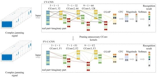
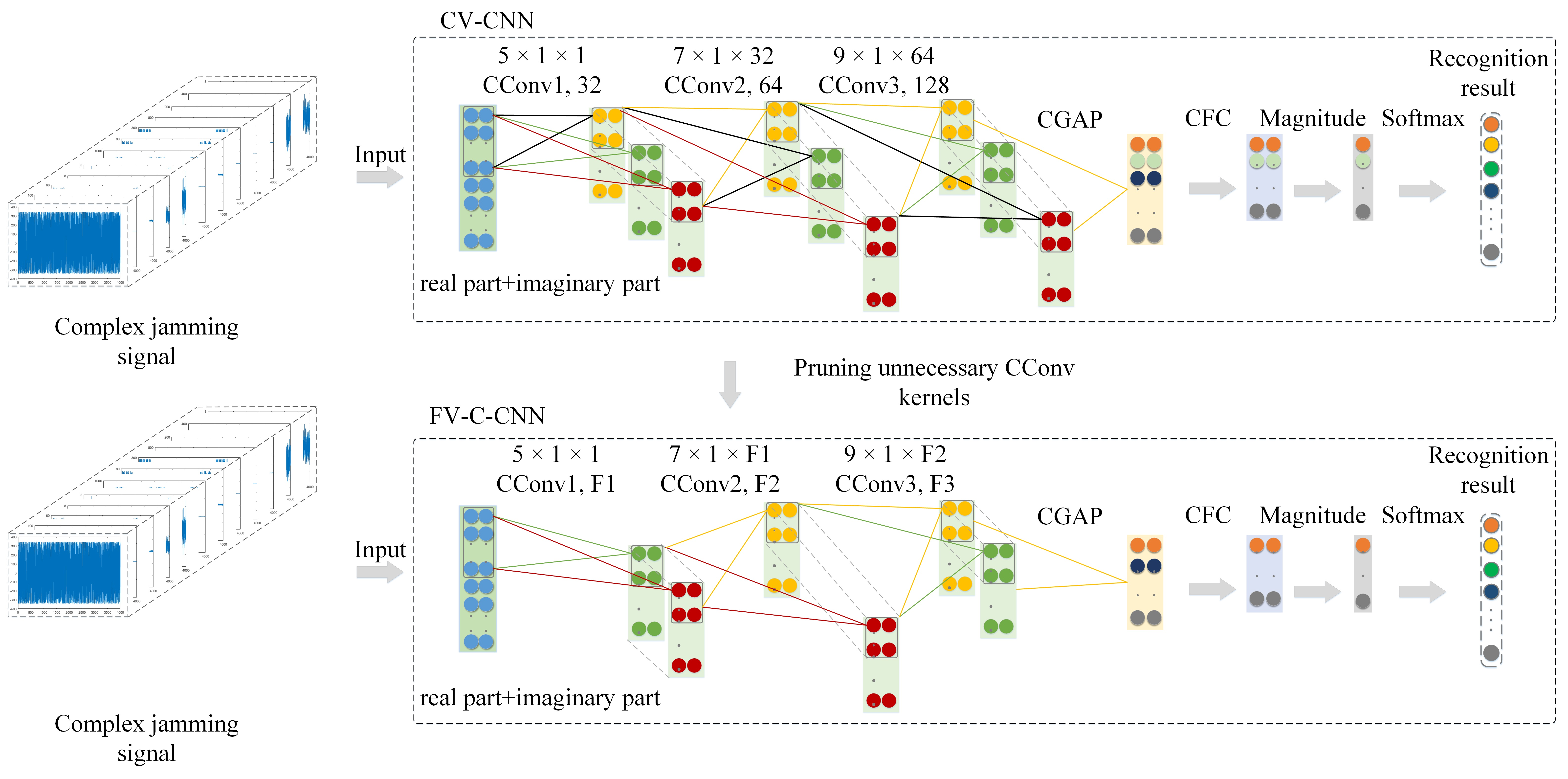
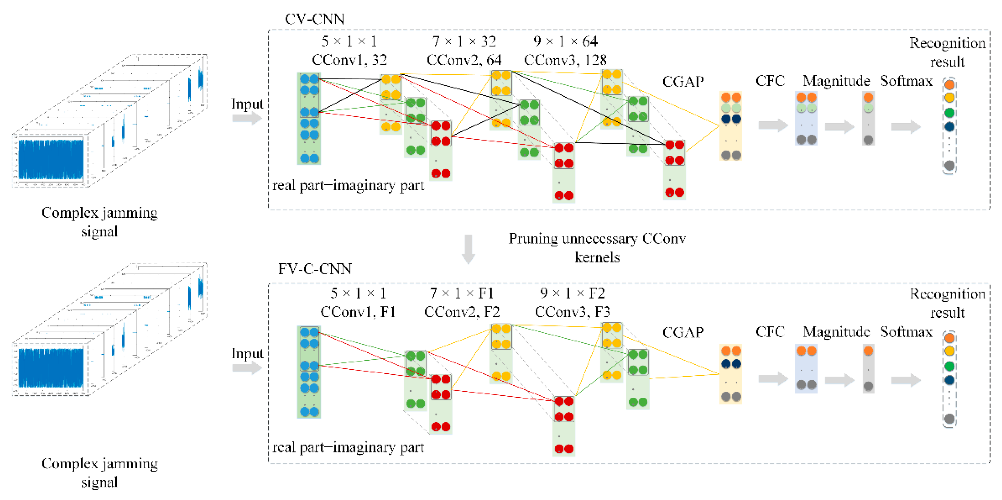
The CV-CNN model can make full use of the information of a radar CV jamming signal. Unfortunately, it is difficult to meet the real-time requirements of radar jamming signal recognition due to the high computational complexity. In order to address this issue, a simple yet effective pruning-based fast CV-CNN (F-CV-CNN) method is proposed; the framework of the F-CV-CNN is shown in Figure 4.

As shown in Figure 4, for CV-CNN, some unnecessary CConv kernels that have less impact on the output can be pruned. This can reduce the complexity of the model, so that the CV-CNN can meet the real-time requirement of jamming signal recognition tasks.

Suppose that $\mathsf{\Omega }=\left\{\left(W^1,b^1\right),\left(W^2,b^2\right),\dots ,\left(W^L,b^L\right)\right\}$ is an over-parameter CV-CNN model for radar jamming signal recognition, where $W\in {ℂ}^{F_l\times F_l\times I_{l-1}\times I_l}$ denotes the CConv kernel, and $\underset{¯}{L}$ is the number of CConv layers. On the given CV jamming dataset $D=\left\{\left(x_1,y_1\right),\left(x_2,y_2\right),\dots ,\left(x_N,y_N\right)\right\}$, the difference between the output $\widehat{y}$ of CV-CNN and the true label y can be evaluated by the loss function $L\left(\mathrm{y},\widehat{y},\mathsf{\Omega }\right)$. Therefore, we need to find the subnetwork ${\mathsf{\Omega }}^{*}$ based on the given over-parameter model $\mathsf{\Omega }$, and make ${\mathsf{\Omega }}^{*}$ meet the minimum increase in $L\left(\mathrm{y},\widehat{y},\mathsf{\Omega }\right)$.

In order to obtain ${\mathsf{\Omega }}^{*}$, we can eliminate the unnecessary parameters of the CV-CNN based on model pruning, which is a simple yet effective method to compress and accelerate the deep learning model.

For model pruning, a suitable CConv kernel importance evaluation method is vitally important. In this work, considering the parameters of the CV-CNN being in complex form and the real-time requirement of the jamming recognition task, the magnitude of CConv is utilized as the importance evaluation criterion. In actual engineering applications, the computational complexity of the magnitude is low, which is more suitable for engineering implementation. The calculation formula of the magnitude is as follows:

$${\mathrm{P}}_{\mathrm{i}}^{\left(\mathrm{l}\right)}=\sqrt{{\left(ℛ({\mathrm{w}}_{\mathrm{i}}^{\left(\mathrm{l}\right)})\right)}^2+{\left(ℐ({\mathrm{w}}_{\mathrm{i}}^{\left(\mathrm{l}\right)})\right)}^2},$$

(19)

where $P_i^{\left(l\right)}$ is the magnitude of the i-th CConv kernel of layer $l$. A smaller $P_i^{\left(l\right)}$ means the less importance of the CConv kernel $w_i^{\left(l\right)}$, and the impact on the CV-CNN is smaller, so it can be eliminated.

By removing the CConv kernel together with their connection feature maps, the computational cost is significantly reduced. Suppose the input jamming feature map for the l-th CConv layer is $a_k^{\left(l-1\right)}\in {ℂ}^{W_{l-1}\times H_{l-1}\times I_{l-1}}$. Through the CConv operation $W^{\left(l\right)}\in {ℂ}^{F_l\times F_l\times I_{l-1}\times I_l}$ in the $l$-th CConv layer, the input CV jamming feature map $a_k^{\left(l-1\right)}$ is then converted into the CV output jamming feature map $a_k^{\left(l\right)}\in {ℂ}^{W_l\times H_l\times I}$. In the $l$-th CConv layer, the total number of multiplication operations of CConv is $2\times F_l\times F_l\times I_{l-1}\times I_l\times W_l\times H_l$. When a certain CConv kernel is eliminated, $2\times F_l\times F_l\times I_{l-1}\times W_l\times H_l$ multiplication operations are reduced in the $l$-th CConv layer. In addition, the corresponding output feature maps are also removed, which further reduces $2\times F_{l+1}\times F_{l+1}\times I_{l+1}\times W_{l+1}\times H_{l+1}$ multiplications in the $l$+1-th CConv layer.

The F-CV-CNN algorithm is a “train, prune, and fine-tune” algorithm, which means that F-CV-CNN can be summarized into three steps: training, pruning, and fine-tuning.

Figure 1 is divided into three parts: training set, validation set, and test set. The training set and validation set are fed into the over-parameter CV-CNN for model training.

Secondly, in the process of pruning, considering that the layer-by-layer iterative fine-tuning pruning strategy is time-consuming, which is not suitable for real-time jamming signal recognition task, a one-shot pruning and fine-tuning is adopted to prune the over-parameter CV-CNN $\mathsf{\Omega }$. The magnitude $P_i^{\left(l\right)}$ of the CConv kernel is calculated layer by layer. Next, in the l-th layer, CConv kernels are sorted according to the value of $P_i^{\left(l\right)}$. Then, $m^l$ CConv kernels with the smallest value of $P_i^{\left(l\right)}$ are pruned, and the corresponding feature maps are removed simultaneously. The pruning algorithm is iteratively carried out layer by layer until all the CConv layers are pruned, and the simplified model ${\mathsf{\Omega }}^{*}$ is obtained.

Finally, in most cases, due to the model pruning, the simplified model ${\mathsf{\Omega }}^{*}$ will have a performance loss compared to the over-parameter model $\mathsf{\Omega }$. Therefore, in order to recover the accuracy loss caused by pruning, we need to fine-tune ${\mathsf{\Omega }}^{*}$. In our work, we adopted a fine-tune measure to train the simplified model ${\mathsf{\Omega }}^{*}$ for fewer epochs at a lower learning rate. Algorithm 1 shows the workflow of the proposed fast CV-CNN.

Algorithm 1: F-CV-CNN method for radar jamming recognition.

1. begin

2.       divide the jamming signal set into training set, validation set, and test set,

3.       input training set and validation set into CV-CNN to train an over-parameterized model $\mathsf{\Omega }$,

4.       iteratively pruning over-parameterized model $\mathsf{\Omega }$ layer by layer:

5.       for$l=1,2,\dots ,L$ do

6.             calculate the magnitude $P_i^{\left(l\right)}$ of each CConv kernel of $l$-th layer

7.             sort all CCon kernels of the $l$-th layer, according to $P_i^{\left(l\right)}$.

8.             remove $m^l$ CConv kernels $w_l^m$ with smaller magnitude in $l$-th layer,

9.             remove the feature maps generated by $w_l^m$.

10.      end

11.      fine-tune the obtain the pruned model ${\mathsf{\Omega }}^{*}$.

12. end

4. Experiments and Results

4.1. Datasets Description

Because linear frequency modulation (line frequency modulation, LFM) signal has the advantages of low peak power and simple modulation method, it has been widely used in the current pulse compression radar system. The expression of the LFM signal is as follows:

$$\mathrm{x}\left(\mathrm{t}\right)=\mathrm{rect}\left(\frac{\mathrm{t}}{\mathrm{T}}\right)\exp \left(\mathrm{j}\mathsf{\pi }\frac{\mathrm{B}}{\mathrm{T}}{\mathrm{t}}^2\right).$$

(20)

Then, 12 kinds of expert-simulated radar jamming signal as experimental datasets were considered to verify the effectiveness of the proposed method, including pure noise, active jamming, and passive jamming. Among them, active jamming includes typical suppression jamming, such as aiming jamming, blocking jamming, sweeping jamming; typical deception jamming such as interrupted sampling repeater jamming (ISRJ) [29]; distance deception jamming [30]; dense false target jamming [31]; smart noise jamming; and passive jamming, such as chaff jamming [11]. In addition, we also considered some composite jamming, such as ISRJ and chaff compound jamming, dense false target and smart noise compound jamming, and distance deception and sweeping compound jamming.

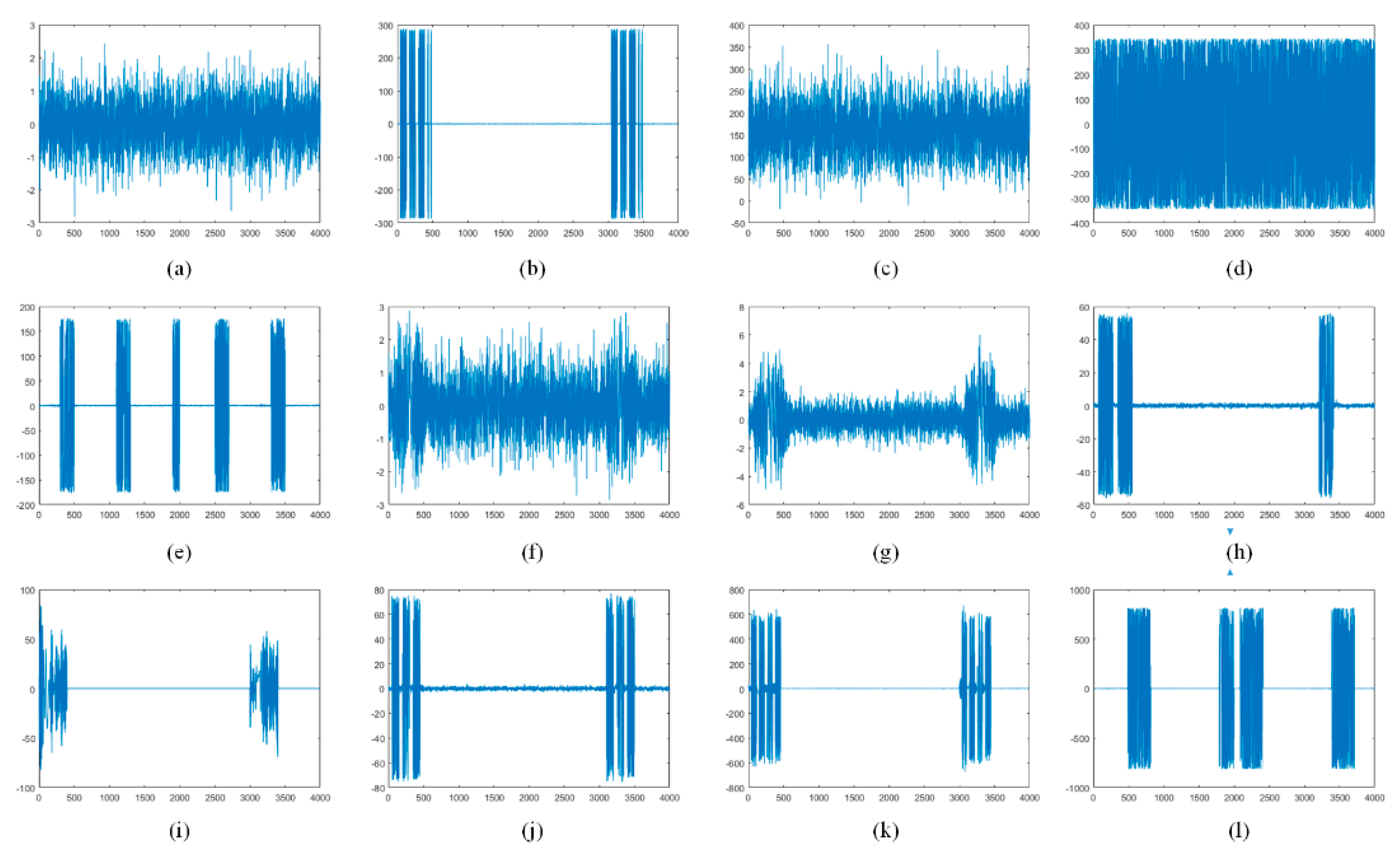
For the simulated radar jamming signal set, each type of radar jamming signal had 500 simulated samples. Each sample had 2000 sampling points, and each sampling point was composed of a real part and imaginary part. Figure 5 shows the waveform of the radar jamming signal in the time domain. The pulse width T of the simulated LFM signal we used was 20$\mathsf{\mu }\mathrm{s}$, the bandwidth $B$ was 10 MHz, and the sampling frequency $f_s$ was 20 MHz. The simulation parameters of the jamming signal were shown in

Table 1. Parameter setting of radar jamming signal simulation.

Jamming	Parameters	Value Range
ISRJ	JNR (dB)	30 to 60
	Sampling duration ($\mu$s)	20 to 40
	Pulse repetition times	30 to 60
Aiming	JNR (dB)	50 to 80
	Bandwidth (MHz)	30 to 60
Blocking	JNR (dB)	10
	Bandwidth (MHz)	4 × 10−5 to 8 × 10−5
Swept	JNR (dB)	1 to 10
	Sweep range (MHz)	0.5 to 2
	Sweep cycle	30 to 60
Distance deception	False target delay range ($\mu$s)	1 to 4
	False target range	1 to 3
Smart noise	JNR (dB)	3 to 5
	Sampling duration ($\mu$s)	1 to 10
	Pulse repetition times	0.5 to 2
Dense false target	Number of false targets	1000 to 2000
	False target delay range ($\mu$s)	20 to 50
	False target range	10 to 20
Chaff	Number of chaff	30 to 60
	Average Doppler frequency	20 to 40
	Doppler parity variance	30 to 60

.

At the same time, we constructed the expert statistical feature (SF) dataset of the radar jamming signal for the comparative experiment, including four time domain features (i.e., skewness, kurtosis, instantaneous amplitude reciprocal, and envelope fluctuation) and four frequency domain features (i.e., additive gaussian white noise factor, maximum value of normalized instantaneous amplitude and frequency, instantaneous phase correlation coefficient, and frequency stability).

4.2. Experimental Setup

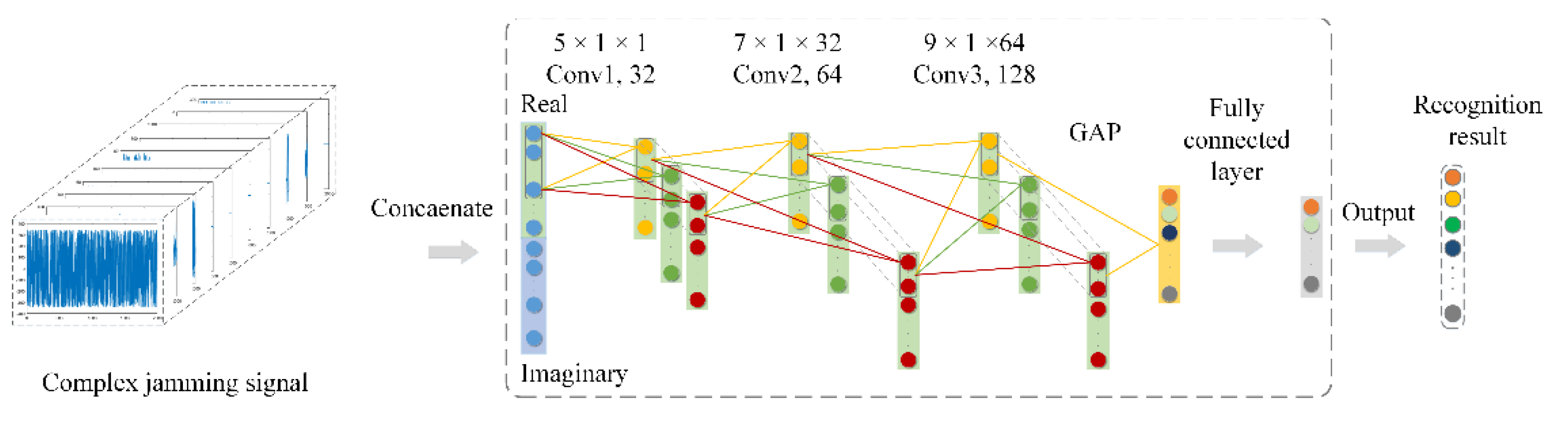
In this study, in order to fully verify the effectiveness of the proposed CV-CNN, the well-designed S-RV-CNN and D-RV-CNN were used for the comparative experiments. The D-RV-CNN consisted of two identical S-RV-CNNs that could extract the real and imaginary features of the CV jamming signal separately. The detailed network structure of RV-CNN is shown in

Table 2. The architecture of the RV-CNN.

Method	Convolution	BN	ReLU	Pooling	Dropout
S-RV-CNN	Input layer
	CConv (5,1,32)	CBN	cReLU	CMaxPooling (2$\times$2)	No
	CConv (7,32,64)	No	cReLU	CMaxPooling (2$\times$2)	No
	CConv (9,64,128)	No	cReLU	CMaxPooling (2$\times$2)	CDropout (50%)
	GAP
	FC
	Output layer
D-RV-CNN	Input layer
	CConv (5,1,32)	CBN	cReLU	CMaxPooling (2$\times$2)	No
	CConv (7,32,64)	No	cReLU	CMaxPooling (2$\times$2)	No
	CConv (9,64,128)	No	cReLU	CMaxPooling (2$\times$2)	CDropout (50%)
	GAP
	Concatenate real and imaginary part features
	FC
	Output layer

.

The S-RV-CNN contained three convolutional layers, three pooling layers, a dropout layer, a BN layer, and a GAP layer. The activation function adopted the ReLU activation function. The convolution step lengths were all set to 1, and the pooling operation adopted a max-pooling operation.

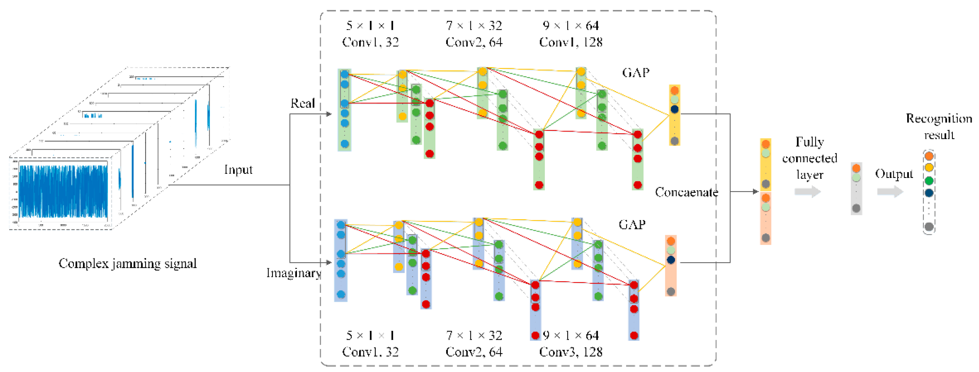
The D-RV-CNN consisted of two identical S-RV-CNNs. The inputs of the two S-RV-CNNs were the real and imaginary parts of the CV jamming signal, which were used to extract the features of the real and imaginary parts separately. The concatenation layer was used to concatenate the real and imaginary part features extracted by two S-RV-CNNs, and then sent the concatenated feature vector as input into the FC layer for feature integration. Finally, the recognition result was obtained by Softmax.

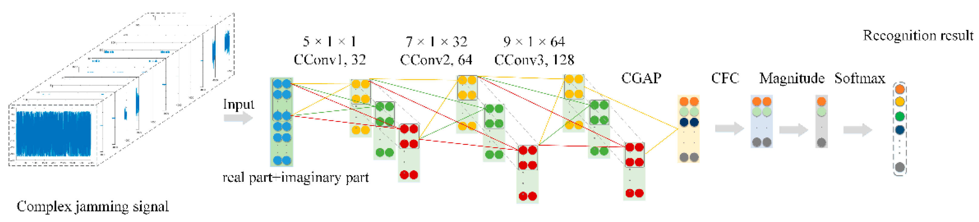
For the proposed CV-CNN, its specific network structure is shown in

Table 3. The architecture of the proposed CV-CNN.

Convolution	BN	ReLU	Pooling	Dropout
Input layer
CConv (5,1,32)	CBN	cReLU	CMaxPooling (2$\times$2)	No
CConv (7,32,64)	No	cReLU	CMaxPooling (2$\times$2)	No
CConv (9,64,128)	No	cReLU	CMaxPooling (2$\times$2)	CDropout (50%)
CGAP
CFC
Magnitude layer
Output layer (Softmax)

. Extending the RV-CNN to the complex domain, the CV-CNN included three CConv layers and CPooling layers, one CDropout layers, a CBN layer, and a CGAP layer. The activation function was also extended from the real domain to the complex domain, adopting the ReLU activation function in complex form.

We divided the CV radar jamming signal used in the experiment into three subsets: training set, validation set, and test set. For each class of radar jamming, we randomly selected 25, 50, 75, 100, and 150 samples per class as the training set, 50 samples per class as the validation set, and the remaining data as the test set.

For the S-RV-CNN, D-RV-CNN, and the CV-CNN, we kept the same hyperparameter settings during the experiment. The learning rate was annealed down from 0.009 to 0.0008, and the batch size and training epochs were set to 64 and 100, respectively.

In addition, we used the SF dataset to train different classifiers as the comparison experiment, i.e., support vector machine (SVM), random forest (RF) [32], decision tree (DT) [33], and K-nearest neighbors (KNN) [34]. The kernel function of the SVM was a radial basis kernel function, the maximum tree depth of the DT was set to 6, the size of the RF was set to 300, and K in KNN was set to 10.

To evaluate the effectiveness of the proposed methods, we used two evaluation metrics, i.e., overall accuracy (OA) and kappa coefficient (K), to evaluate the recognition effect of different methods. OA could be calculated as:

$$\mathrm{OA}=\frac{\mathrm{n}}{\mathrm{N}}\times 100,$$

(21)

The kappa coefficient could be calculated as:

$$\{\begin{array}{c}{\mathrm{p}}_{\mathrm{e}}=\frac{{\mathrm{a}}_1\times {\mathrm{b}}_1+{\mathrm{a}}_2\times {\mathrm{b}}_2+\cdots +{\mathrm{a}}_{12}\times {\mathrm{b}}_{12}}{{\mathrm{N}}^2}\hfill \\ \mathrm{Kappa}=\frac{\mathrm{OA}-{\mathrm{p}}_{\mathrm{e}}}{1-{\mathrm{p}}_{\mathrm{e}}}\hfill \end{array}$$

(22)

where $a_1,a_2,\dots , a_{12}$ denoted the number of test samples for each class jamming signal, and $b_1,b_2,\dots , b_{12}$ denoted the number of correct recognitions of each class jamming signal.

In our work, CV-CNN training and testing, pruning, and other comparative experiments were run on a computer equipped with a 3.4-GHz CPU and a NVIDIA GeForce GTX 1070ti card. All deep learning methods were implemented on the PyCharm Community 2019.1 platform with Pytorch 1.1.0 and CUDA 9.0. In addition, F-CV-CNN was also verified on the NVIDIA Jetson Nano development kit.

4.3. Experimental Results and Performance Analysis

4.3.1. The Recognition Results of CV-CNN

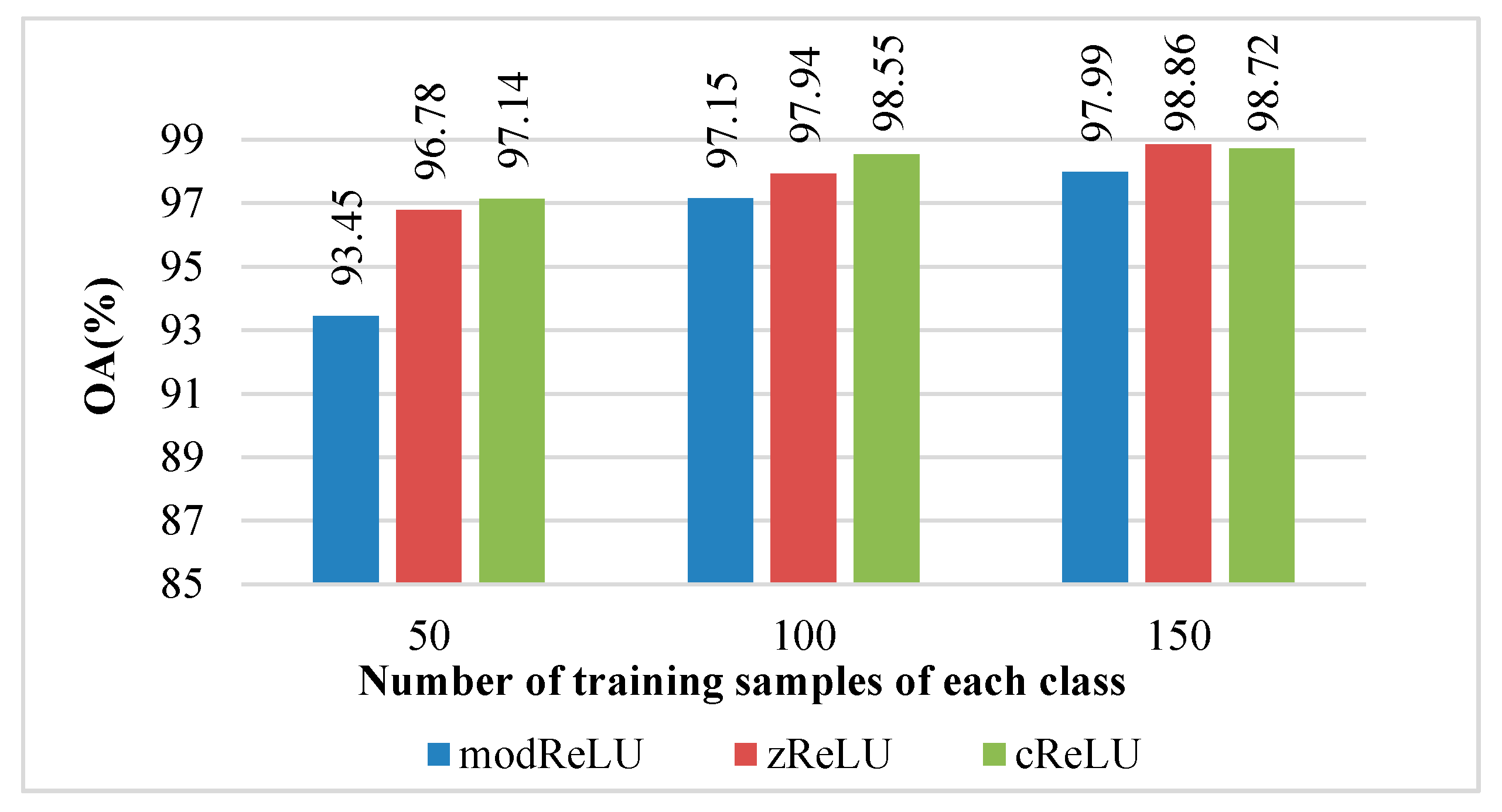
For the proposed CV-CNN, we first considered the impact of different activation function layers and different BN layers on its recognition effect. In this work, three CV activation functions were utilized to explore the influence of different activation functions on the recognition effect of the CV-CNN.

Figure 6 shows the recognition effect of the CV-CNN with different activation functions, i.e., modReLU, zReLU, and cReLU. As shown in Figure 6, under the condition of 50 training samples of each class, the CV-CNN could obtain the recognition accuracy of 93.45%, 96.78%, and 97.14% when using the modReLU, zReLU, and cReLU activation functions, respectively. When the activation function was cReLU, the proposed CV-CNN could achieve the best recognition performance.

The recognition effect of the CV-CNN when adopting different BN layers is shown in

Table 4. Recognition results of CV-CNN with different BN layer.

N	Method	CV-CNN	CV-CNN-RBN	CV-CNN-CBN
50	OA (%)	96.75$\pm$0.64	96.92$\pm$0.55	97.14$\pm$0.70
	K $\times$ 100	96.46$\pm$0.70	96.64$\pm$0.60	96.88$\pm$0.76
100	OA (%)	97.39$\pm$0.77	98.10$\pm$0.40	98.55$\pm$0.34
	K $\times$ 100	97.48$\pm$0.84	97.92$\pm$0.43	98.42$\pm$0.37
150	OA (%)	98.33$\pm$0.30	98.43$\pm$0.48	98.72$\pm$0.19
	K $\times$ 100	98.18$\pm$0.33	98.29$\pm$0.51	98.61$\pm$0.21

. As shown in Table 4, when the BN layer was not introduced in CV-CNN, and when RBN and CBN were used with CNN separately, recognition accuracies of 96.75%, 96.92% and 97.14% can be obtained, respectively. When using the CBN layer, CV-CNN could achieve the best recognition effect.

Similar experimental results could be obtained when each class of training sample was 100 and 150. For CV-CNN, using the cReLU activation function and a CBN layer could achieve better recognition accuracy.

Table 5. Recognition results on radar jamming signal dataset (values ± standard deviation). The best accuracy is highlighted in bold.

N	Method	SF-RBF-SVM	SF-RF-300	SF-DT	SF-KNN	S-RV-CNN	D-RV-CNN	CV-CNN
25	OA(%)	73.44$\pm$1.29	90.26$\pm$0.42	87.80$\pm$1.08	69.40$\pm$0.36	84.85 ± 1.74	84.05$\pm$1.25	95.49$\pm$1.35
	K$\times$100	71.02$\pm$1.41	89.38$\pm$0.46	86.69$\pm$1.18	66.62$\pm$0.39	83.48 ± 1.90	82.61$\pm$1.37	95.08$\pm$1.47
50	OA(%)	79.17$\pm$1.33	90.52$\pm$0.10	88.67$\pm$0.70	71.51$\pm$0.86	90.17 ± 1.93	91.43$\pm$0.88	97.14$\pm$0.70
	K$\times$100	77.28$\pm$1.45	89.65$\pm$0.11	87.64$\pm$0.77	68.93$\pm$0.94	89.27 ± 2.11	90.65$\pm$0.97	96.88$\pm$0.76
75	OA(%)	80.93$\pm$0.66	90.71$\pm$0.40	89.84$\pm$0.29	72.47$\pm$0.32	90.79 ± 1.54	93.24$\pm$1.71	98.24$\pm$0.33
	K$\times$100	79.20$\pm$0.72	89.87$\pm$0.44	88.92$\pm$0.31	69.97$\pm$0.34	89.96 ± 1.68	92.63$\pm$1.86	98.08$\pm$0.36
100	OA(%)	82.46$\pm$0.29	91.52$\pm$0.12	89.27$\pm$0.17	72.88$\pm$0.53	94.20 ± 1.39	95.24$\pm$0.86	98.55$\pm$0.34
	K$\times$100	80.86$\pm$0.32	90.75$\pm$0.13	88.30$\pm$1.8	70.42$\pm$0.58	93.67 ± 1.52	94.81$\pm$0.94	98.42$\pm$0.37
150	OA(%)	83.56$\pm$0.26	91.63$\pm$0.18	89.89$\pm$0.71	73.30$\pm$0.52	96.10 ± 1.28	96.27$\pm$0.22	98.72$\pm$0.19
	K$\times$100	82.07$\pm$0.29	90.87$\pm$0.19	88.97$\pm$0.77	70.87$\pm$0.57	95.75 ± 1.40	95.93$\pm$0.25	98.61$\pm$0.21
	C1	99.66 ± 0.67	100.00$\pm$0.00	100.00$\pm$0.00	100.00$\pm$0.00	100 ± 0.00	99.93$\pm$0.13	100.00$\pm$0.00
	C2	76.20$\pm$2.5	96.80$\pm$1.34	90.97$\pm$2.64	26.45$\pm$3.38	97.93± 3.81	98.27$\pm$1.51	98.93$\pm$0.53
	C3	99.53$\pm$0.16	100.00$\pm$0.00	100.00$\pm$0.00	99.26$\pm$0.14	100 ± 0.00	100.00$\pm$0.00	100.00$\pm$0.00
	C4	98.47$\pm$1.36	100.00$\pm$0.00	100.00$\pm$0.00	100.00$\pm$0.00	100 ± 0.00	99.87$\pm$0.16	99.73$\pm$0.39
	C5	98.07$\pm$1.31	100.00$\pm$0.00	100.00$\pm$0.00	100.00$\pm$0.00	90.87 ± 3.04	92.47$\pm$3.02	98.27$\pm$0.83
	C6	97.73$\pm$1.06	97.54$\pm$1.41	98.51$\pm$0.49	98.46$\pm$0.97	94.07 ± 2.66	94.20$\pm$3.15	95.13$\pm$2.09
	C7	98.20$\pm$0.62	97.09$\pm$0.33	95.94$\pm$0.94	84.45$\pm$1.67	94.07 ± 3.97	92.13$\pm$2.54	96.93$\pm$1.54
	C8	46.27$\pm$5.99	62.97$\pm$2.49	54.97$\pm$4.87	21.26$\pm$2.33	93.67 ± 4.42	97.06$\pm$1.51	99.73$\pm$0.25
	C9	100.00$\pm$0.00	100.00$\pm$0.00	100.00$\pm$0.00	94.69$\pm$1.15	100 ± 0.00	100.00$\pm$0.00	98.40$\pm$1.02
	C10	39.93$\pm$7.21	56.46$\pm$2.92	54.69$\pm$1.99	23.09$\pm$2.42	95.27 ± 4.31	94.47$\pm$2.65	99.73$\pm$0.24
	C11	51.60$\pm$5.24	88.74$\pm$2.84	83.60$\pm$2.37	33.26$\pm$3.34	98.73 ± 1.50	98.73$\pm$0.88	98.60$\pm$0.77
	C12	97.07$\pm$1.97	100.00$\pm$0.00	100.00$\pm$0.00	98.69$\pm$1.00	88.6 0 ± 4.83	88.07$\pm$3.15	99.47$\pm$0.62

shows the detailed results of the proposed CV-CNN, and the best recognition accuracy is highlighted in bold. In Table 4, C1–C12 represent pure noise, ISRJ, aiming jamming, blocking jamming, sweeping jamming, distance deception jamming, dense false target jamming, smart noise, chaff jamming, chaff and ISRJ compound jamming, dense false target and smart noise compound jamming, distance deception, and sweeping compound jamming, respectively. From Table 4, one can see that CV-CNN demonstrated its best recognition performance in terms of OA and K.

Under the condition of 25 training samples of each class, the CV-CNN improved the OA by 10.11% compared to the D-RV-CNN. In addition, the CV-CNN also outperformed the SF-classifier methods. In the case of 50 training samples per class, the CV-CNN exhibited the OA over D-RV-CNN and SF-RF, with improvements of 5.73% and 6.64%.

In addition, experiments with 75, 100, and 150 training samples of each class were also conducted to further demonstrate the effectiveness of our method, the results are also shown in Table 5. It could be seen from Table 5 that the CV-CNN achieved the best recognition performance, with 75, 100, and 150 training samples per class, which fully demonstrated the effectiveness of our proposed CV-CNN.

Table 6. Comparison of recognition accuracy between CV-CNN and other CNN-based methods. The best accuracy is highlighted in bold.

N	Method	S-RV-CNN	D-RV-CNN	2D-CNN [21]	1D-CNN [21]	CV-CNN
50	OA (%)	90.17$\pm$1.93	91.43$\pm$0.88	87.83$\pm$1.84	91.95$\pm$2.19	97.16$\pm$0.53
	K $\times$ 100	89.27$\pm$2.11	90.65$\pm$0.97	86.72$\pm$2.01	91.21$\pm$2.39	96.90$\pm$0.58
100	OA (%)	94.20$\pm$1.39	95.24$\pm$0.86	89.88$\pm$0.47	96.97$\pm$0.88	98.24$\pm$0.36
	K $\times$ 100	93.67$\pm$1.52	94.81$\pm$0.94	88.97$\pm$0.52	96.69$\pm$0.96	98.08$\pm$0.39
150	OA (%)	96.10$\pm$1.28	96.27$\pm$0.22	91.33$\pm$1.29	97.34$\pm$0.37	98.76$\pm$0.23
	K $\times$ 100	95.75$\pm$1.40	95.93$\pm$0.25	90.55$\pm$1.40	97.10$\pm$0.41	98.64$\pm$0.25

shows the results of the proposed method and some previous CNN-based comparative methods. For the detailed network structure of 2D-CNN and 1D-CNN, please refer to [21].

With 50 training samples per class, the CV-CNN achieved a recognition accuracy of 97.16%, which improved by 9.33% and 5.21% in terms of OA compared with the 2D-CNN and 1D-CNN, respectively. With 100 training samples per class, the CV-CNN could achieve a recognition accuracy of 98.24%. Compared with the 2D-CNN (89.88%) and 1D-CNN (96.97%) in [21], the CV-CNN achieved an improvement of 8.36% and 1.27%, respectively. In the case of 150 training samples per class, CV-CNN also achieved the highest recognition accuracy. Compared with 2D-CNN and 1D-CNN, the proposed CV-CNN improved the recognition accuracy of 7.43% and 1.43%, respectively.

Under different Dropout rates, the recognition accuracy of CV-CNN was shown in the

Table 7. CV-CNN recognition accuracy under different dropout rates. The best accuracy is highlighted in bold.

N	Rate	0.1	0.3	0.5	0.7	0.9
50	OA (%)	96.33$\pm$0.87	97.10$\pm$0.86	97.14$\pm$0.70	97.41$\pm$0.56	96.99$\pm$0.61
	K $\times$ 100	96.00$\pm$0.94	96.84$\pm$0.94	96.88$\pm$0.76	97.18$\pm$0.61	96.72$\pm$0.66
100	OA (%)	98.09$\pm$0.85	98.41$\pm$0.44	98.55$\pm$0.34	98.36$\pm$0.25	97.86$\pm$0.22
	K $\times$ 100	97.91$\pm$0.09	98.27$\pm$0.48	98.42$\pm$0.37	98.21$\pm$0.27	97.67$\pm$0.24

. It could be found that when the dropout rate was small, there was an over-fitting phenomenon for CV-CNN, which led to a decrease in the recognition accuracy of CV-CNN. When the dropout rate was high, the recognition accuracy of CV-CNN would also decrease due to the high proportion of randomly discarded neurons. Therefore, a moderate Dropout rate should be selected. In our experiment, we set the dropout rate to 0.5.

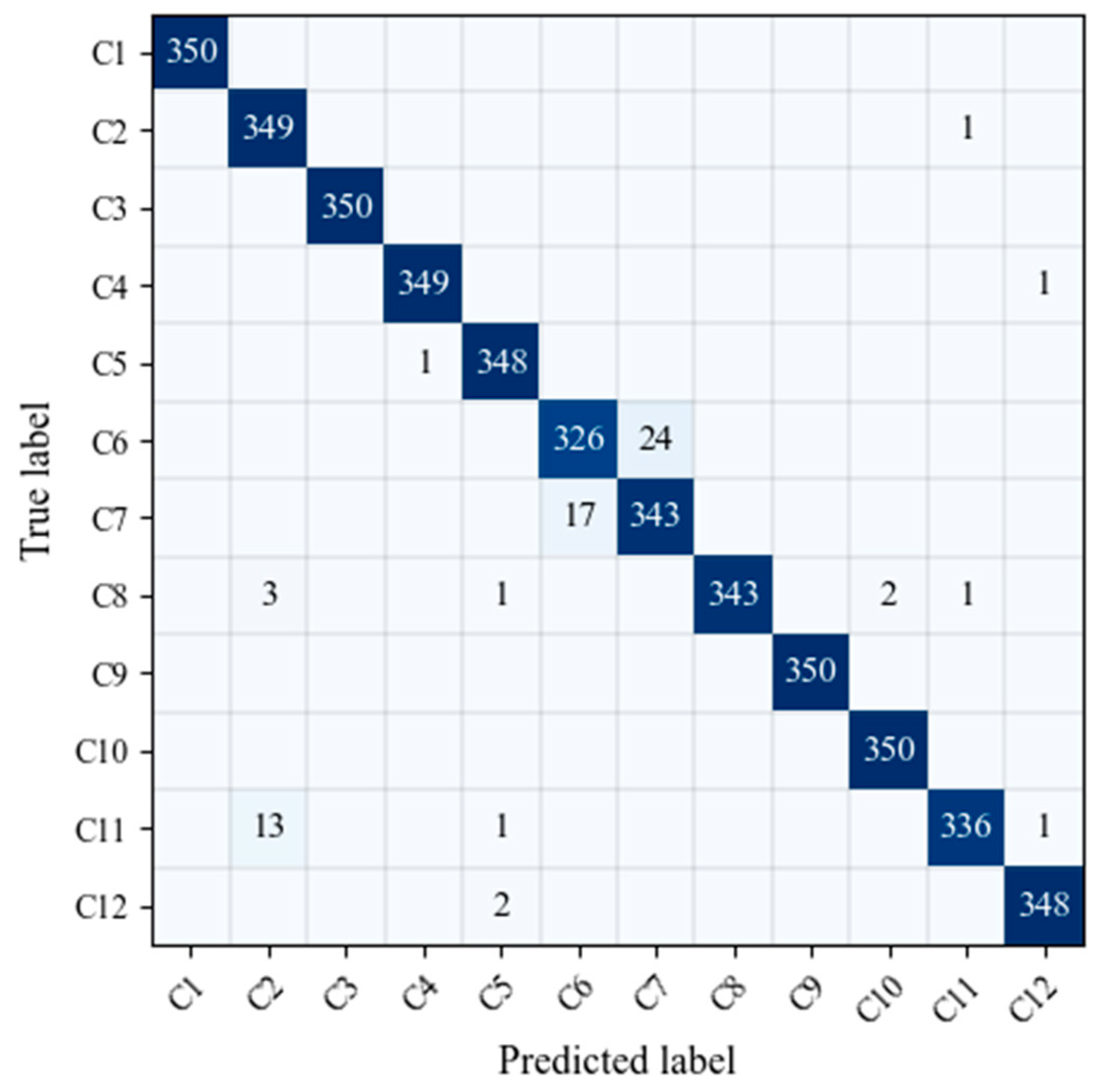
It could be found from Figure 7 that CV-CNN can achieve a better recognition of jamming signal, but it is easy to confuse C6 (distance false targets) and C7 (dense false targets). The reason for the above phenomenon was mainly due to the fact that the simulation parameters of distance false targets and dense false targets were the same except for the number of false targets. As a result, the two types of jamming signal had a certain degree of similarity, and it is easy to confuse the two.

4.3.2. The Recognition Results of F-CV-CNN

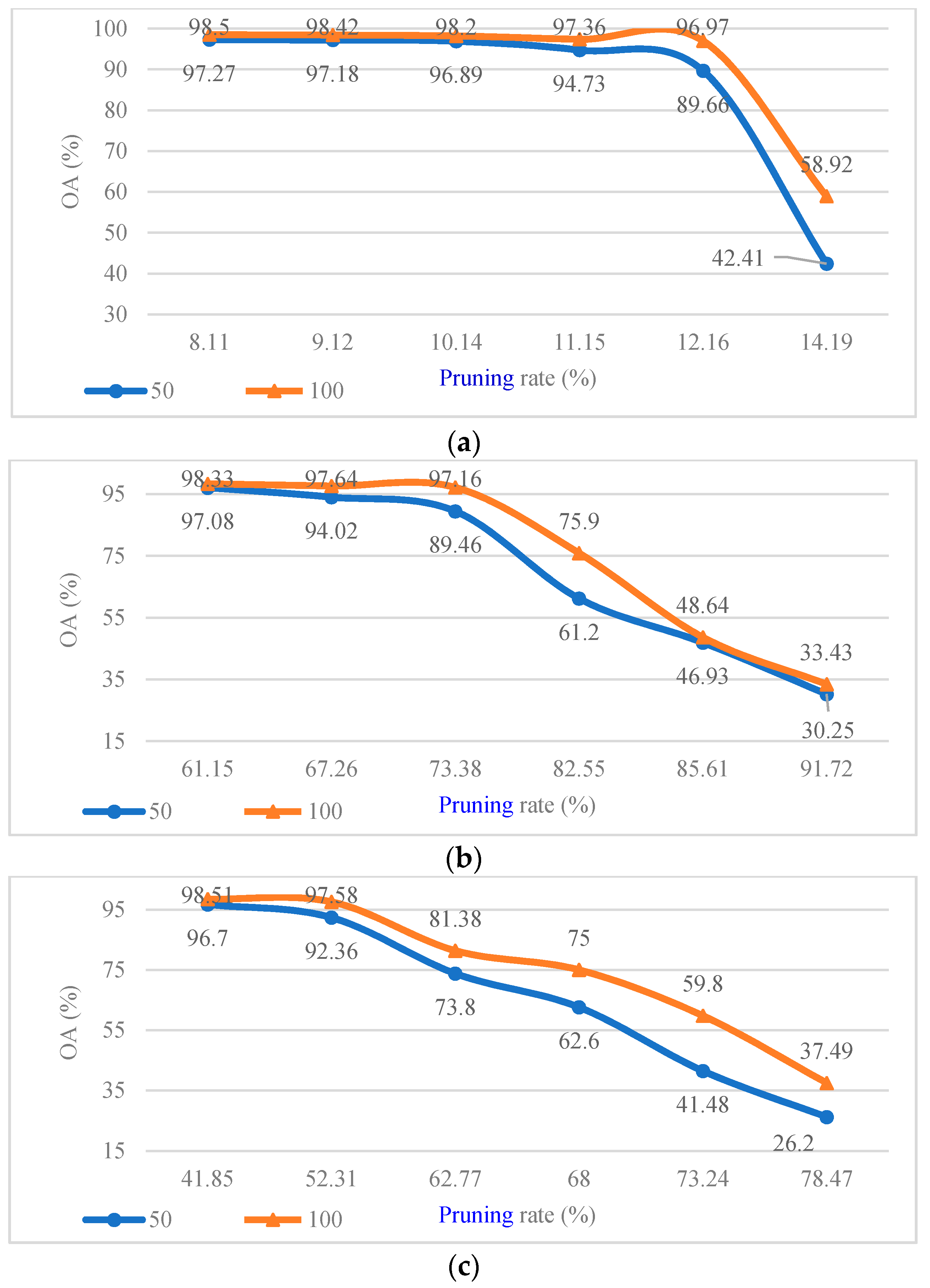
Considering that the CConv kernels in different layers of CV-CNN had different sensitivity to pruning, we first analyzed the pruning sensitivity of CV-CNN. The pruning sensitivity curves of different CConv layers in CV-CNN are shown in Figure 8, with 50 and 100 training samples per class. As shown in Figure 8, for the first layer of CConv, when the pruning rate was 14.19%, the model performance after pruning began to decline; for the third layer, when the pruning rate reached 62.77%, the model performance after pruning began to decline. In summary, for the CV-CNN used in the experiment, the pruning sensitivity of the second layer was smaller than that of the first and third layers. In the same CConv layer, the CV-CNN that was trained by more training samples had stronger pruning robustness.

In this subsection, the over-parameter CV-CNN and the simplified model obtained by the F-CV-CNN algorithm were expressed as $\mathsf{\Omega }$ and ${\mathsf{\Omega }}^{*}$, respectively. First, with 50, 100, and 150 training samples for each class, $\mathsf{\Omega }$ was trained separately. Then the F-CV-CNN algorithm was carried out on the $\mathsf{\Omega }$ to obtain ${\mathsf{\Omega }}^{*}$.

Table 8. Recognition results of F-CV-CNN on radar jamming signal dataset (values ± standard deviation).

	Pruning Rate	Fine-tune	0%	42%	56%	70%	74%	85%	92%
N
50		No	97.14$\pm$0.70	96.74$\pm$1.37	96.74$\pm$1.28	96.73$\pm$1.33	96.89$\pm$1.34	73.75$\pm$15.14	68.3$\pm$14.17
		Yes	97.14$\pm$0.70	97.47$\pm$0.64	97.50$\pm$0.66	97.42$\pm$0.84	97.59$\pm$0.72	93.85$\pm$4.27	90.66$\pm$5.65
100		No	98.55$\pm$0.34	98.54$\pm$0.30	98.48$\pm$0.34	98.53$\pm$0.41	98.36$\pm$0.46	81.25$\pm$8.66	83.03 $\pm$9.29
		Yes	98.55$\pm$0.34	98.75$\pm$0.20	98.78$\pm$0.10	98.76$\pm$0.14	98.72$\pm$0.21	98.27$\pm$0.81	97.85$\pm$0.99
150		No	98.72$\pm$0.19	98.62$\pm$0.30	98.73$\pm$0.15	98.78$\pm$0.17	98.72$\pm$0.13	94.42$\pm$4.23	94.22$\pm$4.20
		Yes	98.72$\pm$0.19	98.91$\pm$0.19	98.90$\pm$0.22	98.94$\pm$0.21	98.94$\pm$0.25	98.78$\pm$0.30	98.61$\pm$0.19

shows the recognition results of ${\mathsf{\Omega }}^{*}$ under different pruning rates. As shown in Table 8, when the pruning ratio is low, the performance loss caused by model pruning can be ignored. However, with the increase of the pruning rate, the recognition performance of ${\mathsf{\Omega }}^{*}$ continues to decline. When there are 50 training sample for each class and the pruning ratio is 85%, the recognition accuracy of ${\mathsf{\Omega }}^{*}$ was reduced from 97.14% to 73.75% compared with $\mathsf{\Omega }$. Similarly, when the number of training samples for each class was 100 and 150, the recognition accuracy of ${\mathsf{\Omega }}^{*}$ also dropped to 81.25% and 94.42%, respectively. From Table 8, one could also find the same conclusions as the previous analysis, i.e., the more training samples, the smaller performance loss of ${\mathsf{\Omega }}^{*}$.

In order to restore the performance of ${\mathsf{\Omega }}^{*}$, a fine-tune post-processing operation was required. The specific operation was to train 15 epochs at a low learning rate of 0.0001. The experimental results of fine-tune post-processing on ${\mathsf{\Omega }}^{*}$ are also shown in Table 8. As shown in Table 8, the fine-tune post-processing could restore the recognition performance of ${\mathsf{\Omega }}^{*}$ to a certain extent.

With a pruning rate of 92% and 50 training samples per class, the recognition performance of ${\mathsf{\Omega }}^{*}$ after fine-tune processing was restored to 90.66%. Compared with $\mathsf{\Omega }$, the performance of ${\mathsf{\Omega }}^{*}$ had dropped by 6.48%. However, in the case of 100 and 150 training samples per class, the performance of ${\mathsf{\Omega }}^{*}$ at a pruning rate of 92% could also be restored well through fine-tune processing. The results also showed that for the deep learning model, the more training samples, the stronger the robustness of the model.

In order to better show the effectiveness of the F-CV-CNN algorithm, we tested the inference time of ${\mathsf{\Omega }}^{*}$ on NVIDIA Jetson Nano, which is used for real-time jamming recognition in our work.

Table 9. The FLOPs and inference time for F-CV-CNN.

Pruning Rate	0%	42%	56%	70%	74%	85%	92%
FLOPs (M)	202.85	130.75	98.48	66.21	51.22	33.17	17.00
Nano time (ms)	87.76	79.59	74.25	57.53	41.17	33.38	28.91

showed the floating-point operations (FLOPs) and inference time.

With the increase of the pruning rate, the FLOPs of ${\mathsf{\Omega }}^{*}$ continued to decrease, and the inference time also continued to decrease. When the pruning rate was 92%, the FLOPs of ${\mathsf{\Omega }}^{*}$ were reduced by 91% compared with the $\mathsf{\Omega }$, and the inference time was also reduced by 67%. The experimental results also fully illustrated the effectiveness of the F-CV-CNN algorithm.

4.3.3. The Recognition of Radar Jamming and Normal Signal

In real application, it is necessary to recognize the radar normal signal and jamming signal at the same time. Therefore, in this subsection, the effectiveness of the proposed CV-CNN was tested on a dataset which contained radar jamming and normal signals.

The radar jamming signals were the signals in Section 4.1, which contained twelve types of radar jamming signals. Furthermore, the normal radar signals were generated based on Equation (20), and they were used as the 13th type of the radar jamming and normal signal dataset. The pulse width T was 20 μs, and bandwidth B was 10 MHz, and the sampling rate was 20 MHz. For the normal radar signals, there were 500 simulated samples. Each sample had 2000 sampling points, and each sampling point was composed of a real part and an imaginary part.

Table 10. Recognition results on radar jamming and normal signal dataset (values ± standard deviation). The best accuracy is highlighted in bold.

N	Method	RF-300	DT	S-RV-CNN	D-RV-CNN	CV-CNN
50	OA (%)	75.99$\pm$0.99	58.83$\pm$1.44	88.33$\pm$2.06	91.30 $\pm$2.35	95.92$\pm$0.65
	K$\times$100	73.99$\pm$1.05	55.40$\pm$1.56	87.35$\pm$2.23	90.57$\pm$2.54	95.58$\pm$0.70
	C13	58.04$\pm$5.97	35.20$\pm$3.36	84.00$\pm$4.56	85.85$\pm$5.00	89.60$\pm$4.07
100	OA (%)	80.48$\pm$0.16	64.17$\pm$0.53	93.86$\pm$1.00	94.14$\pm$1.16	97.66$\pm$0.62
	K$\times$100	78.86$\pm$0.18	61.18$\pm$0.57	93.35$\pm$1.08	93.65$\pm$1.26	97.47$\pm$0.67
	C13	65.60$\pm$1.91	42.70$\pm$2.56	87.43$\pm$3.25	89.94$\pm$2.11	91.20$\pm$3.40
150	OA (%)	82.28$\pm$0.39	67.09$\pm$1.06	94.83$\pm$1.48	95.44$\pm$1.25	98.18$\pm$0.53
	K$\times$100	80.80$\pm$0.42	64.35$\pm$1.15	94.40$\pm$1.60	95.07$\pm$1.35	98.03$\pm$0.58
	C1	100.00$\pm$0.00	69.20$\pm$5.10	100.00$\pm$0.00	100.00$\pm$0.00	100.00$\pm$0.00
	C2	64.91$\pm$0.78	40.29$\pm$5.52	99.94$\pm$0.44	99.73$\pm$0.39	99.07$\pm$0.61
	C3	100.00$\pm$0.00	99.20$\pm$0.49	100.00$\pm$0.00	100.00$\pm$0.00	100.00$\pm$0.00
	C4	100.00$\pm$0.00	84.51$\pm$1.57	99.87$\pm$0.27	100.00$\pm$0.00	100.00$\pm$0.00
	C5	100.00$\pm$0.00	97.37$\pm$0.71	90.53$\pm$4.48	87.93$\pm$8.54	99.00$\pm$0.37
	C6	81.94$\pm$1.59	44.57$\pm$4.92	91.67$\pm$4.26	90.80$\pm$0.95	92.67$\pm$3.11
	C7	77.14$\pm$2.13	39.71$\pm$3.31	95.07$\pm$3.90	90.47$\pm$2.94	95.93$\pm$1.48
	C8	43.03$\pm$1.55	35.43$\pm$2.18	88.33$\pm$6.20	93.73$\pm$5.57	99.33$\pm$0.42
	C9	100.00$\pm$0.00	96.06$\pm$0.55	99.73$\pm$0.39	99.93$\pm$0.13	99.93$\pm$0.13
	C10	36.86$\pm$4.54	33.49$\pm$2.55	89.33$\pm$6.67	94.33$\pm$2.23	99.93$\pm$0.47
	C11	99.71$\pm$0.26	87.94$\pm$4.20	99.07$\pm$0.61	97.73$\pm$1.85	97.20$\pm$2.19
	C12	100.00$\pm$0.00	96.57$\pm$1.39	87.67$\pm$3.09	92.93$\pm$2.31	99.13$\pm$0.16
	C13	66.00$\pm$1.43	47.89$\pm$2.80	92.13$\pm$2.09	93.20$\pm$3.64	94.80$\pm$1.55

shows the experimental results of the proposed method to perform recognition for normal radar signals and jamming signals, where C13 represents the normal radar signal. From Table 10, one can see that CNN-based methods (i.e., S-RV-CNN, D-RV-CNN, and CV-CNN) obtained better recognition performance compared with tradition machine learning methods (i.e., random forest and decision tree). For CNN-based methods, with 50 training samples for each class, the recognition accuracy of the CV-CNN for normal radar signals was 89.60%, which was 5.6% and 3.75% higher than that of the S-RV-CNN (84.00%) and D-RV-CNN (85.85%), respectively.

Moreover, with 100 training samples per class, the CV-CNN improved the recognition accuracy by 3.77% and 1.26% compared with the S-RV-CNN and D-RV-CNN, respectively. With 150 training samples per class, the CV-CNN also achieved the highest recognition accuracy, and the recognition accuracy for normal radar signals reached 94.80%, which further verified the effectiveness of the proposed CV-CNN.

5. Conclusions

In this paper, we proposed a CV-CNN for radar jamming signal recognition which extends the network parameters from real number to complex number. Through CConv, CPooling, CBN layer, and so on, the unique information of the CV jamming data can be better utilized. Experimental results show that our proposed method can better identify CV jamming signals, and its recognition performance was further improved, with the improvements of 11.44% in terms of OA when there are 25 training samples per class.

In addition, in order to deal with the issue of over parameters and poor real-time performance, the F-CV-CNN algorithm was proposed. Based on filter-level filter pruning, unnecessary CConv kernels were pruned to reduce the number of parameters and calculations of CV-CNN so that the CV-CNN meets the real-time requirements of interference signal recognition tasks. After pruning the F-CV-CNN, FLOPs can be reduced by up to 91% compared with CV-CNN, and the inference time can be reduced by 67%.

Furthermore, the effectiveness of the proposed CV-CNN was also tested on a dataset which contained radar jamming and normal signals. The results showed that the CV-CNN worked well on the recognition of radar jamming and normal signals at the same time.

For radar jamming signal recognition, we usually face a problem of limited training samples. Due to a large number of learnable parameters, this problem is serious when deep learning-based methods are used for radar jamming signal recognition. Therefore, in the near future, deep CV CNN-based recognition with limited training samples is the next move of our research.

References

1. Liu, N.; Zhang, Y. A survey of radar ECM and ECCM. IEEE Trans. Aerosp. Electron. Syst. 1995, 27, 1110–1120. [Google Scholar]
2. Feng, D.; Xu, L.; Pan, X.; Wang, X. Jamming wideband radar using interrupted-sampling repeater. IEEE Trans. Aerosp. Electron. Syst. 2017, 53, 1341–1354. [Google Scholar] [CrossRef]
3. Huang, G.; Yang, L. A radar anti-jamming technology based on blind source separation. In Proceedings of the 7th International Conference on Signal Processing, Beijing, China, 31 August–4 September 2004. [Google Scholar]
4. Greco, M.; Gini, F.; Farina, A. Radar detection and classification of jamming signal belonging to a cone class. IEEE Trans. Signal Process. 2008, 56, 1984–1993. [Google Scholar] [CrossRef]
5. Bandiera, F.; Farina, A.; Orlando, D.; Ricci, G. Detection algorithms to discriminate between radar targets and ECM signal. Trans. Signal Process. 2010, 58, 5985–5993. [Google Scholar] [CrossRef]
6. Zhao, S.; Zhou, Y.; Zhang, L.; Tang, S. Discrimination between radar targets and deception jamming in distributed multiple-radar architectures. IET Radar Sonar Navig. 2011, 5, 12–22. [Google Scholar] [CrossRef]
7. Hao, Z.; Yu, W.; Chen, W. Recognition method of dense false targets jamming based on time-frequency atomic decomposition. J. Eng. 2019, 2019, 6354–6358. [Google Scholar] [CrossRef]
8. Liu, Y.; Wang, W.; Pan, X.; Dai, D.; Feng, D. A-frequency-domain three-stage algorithm for active deception jamming against synthetic aperture radar. IET Radar Sonar Navig. 2014, 8, 639–646. [Google Scholar] [CrossRef]
9. Ma, X.; Qin, J.; Li, J. Pattern recognition-based method for radar anti-deceptive jamming. J. Syst. Eng. Electron. 2005, 4, 802–805. [Google Scholar]
10. Tian, X.; Tang, B.; Gui, G. Product spectrum matrix feature extraction and recognition of radar deception jamming. Int. J. Electron. 2013, 100, 1621–1629. [Google Scholar] [CrossRef]
11. Liu, Y.; Xing, S.; Li, Y.; Hou, D.; Wang, X. Jamming recognition method based on the polarization scattering characteristics of chaff clouds. IET Radar Sonar Navig. 2017, 11, 1689–1699. [Google Scholar] [CrossRef]
12. Qin, F.; Meng, J.; Du, J.; Ao, F.; Zhou, Y. Radar jamming effect evaluation based on AdaBoost combined classification model. In Proceedings of the 2013 IEEE 4th International Conference on Software Engineering and Service Science, Beijing, China, 23–25 May 2013; pp. 910–913. [Google Scholar]
13. Gao, M.; Li, H.; Jiao, B.; Hong, Y. Simulation research on classification and identification of typical active jamming against LFM radar. In Proceedings of the 11th International Conference on Signal Processing Systems. International Society for Optics and Photonics, Chengdu, China, 31 December 2019. [Google Scholar]
14. Schmidhuber, J. Deep learning in neural networks: An overview. Neural Netw. 2015, 61, 85–117. [Google Scholar] [CrossRef] [PubMed] [Green Version]
15. LeCun, Y.; Bengio, Y.; Hinton, G. Deep learning. Nature 2015, 521, 436–444. [Google Scholar] [CrossRef] [PubMed]
16. Wang, Y.; Sun, B.; Wang, N. Recognition of radar active-jamming through convolutional neural networks. IET J. Eng. 2019, 2019, 7695–7697. [Google Scholar] [CrossRef]
17. Liu, Q.; Zhang, W. Deep learning and recognition of radar jamming based on CNN. In Proceedings of the 2019 12th International Symposium on Computational Intelligence and Design, Hangzhou, China, 14–15 December 2019; pp. 208–212. [Google Scholar]
18. Qu, Q.; Wei, S.; Liu, S.; Liang, J. Jamming recognition networks for radar compound suppression jamming signal. IEEE Trans. Veh. Technol. 2020, 69, 15035–15045. [Google Scholar] [CrossRef]
19. Wu, Z.; Zhao, Y.; Yin, Z.; Luo, H. Jamming signal classification using convolutional neural network. In Proceedings of the 2017 IEEE International Symposium on Signal Processing and Information Technology, Bilbao, Spain, 18–20 December 2017; pp. 62–67. [Google Scholar]
20. Andriyanov, N.; Dementiev, V.; Gladkikh, A. Analysis of the Pattern Recognition Efficiency on Non-Optical Images. In Proceedings of the 2021 IEEE Ural Symposium on Biomedical Engineering, Radioelectronics and Information Technology (USBEREIT), Online, 13–14 May 2021; pp. 319–323. [Google Scholar]
21. Shao, G.; Chen, Y.; Wei, Y. Convolutional neural network-based radar jamming signal classification with sufficient and limited samples. IEEE Access 2020, 8, 80588–80598. [Google Scholar] [CrossRef]
22. Nikias, C.L.; Raghuveer, M.R. Bispectrum estimation: A digital signal processing framework. Proc. IEEE. 1987, 75, 869–891. [Google Scholar] [CrossRef]
23. Li, J.; Shen, Q.; Yan, H. Signal feature analysis and experimental verification of radar deception jamming. In Proceedings of the 2011 IEEE CIE International Conference on Radar, Chengdu, China, 24–27 October 2011; pp. 230–233. [Google Scholar]
24. Zhou, H.; Dong, C.; Wu, R.; Xu, X.; Guo, Z. Feature fusion based on Bayesian decision theory for radar deception jamming recognition. IEEE Access 2021, 9, 16296–16304. [Google Scholar] [CrossRef]
25. Cheng, Y.; Wang, D.; Zhou, P.; Zhang, T. A Survey of model compression and acceleration for deep neural networks. arXiv 2017, arXiv:1710.09282. [Google Scholar]
26. He, Y.; Zhang, X.; Sun, J. Channel pruning for accelerating very deep neural networks. In Proceedings of the 2017 IEEE International Conference on Computer Vision, Venice, Italy, 22–29 October 2017. [Google Scholar]
27. He, Y.; Liu, P.; Wang, Z.; Hu, Z.; Yang, Y. Filter pruning via geometric median for deep convolutional neural networks acceleration. In Proceedings of the IEEE Conference on Computer Vision and Pattern Recognition, Long Beach, CA, USA, 16–20 June 2019; pp. 4340–4349. [Google Scholar]
28. Wang, W.; Fu, C.; Guo, J.; Cai, D.; He, X. COP: Customized deep model compression via regularized correlation-based filter-level pruning. arXiv 2019, arXiv:1906.10337. [Google Scholar]
29. Wu, Q.; Zhao, F.; Ai, X.; Liu, X.; Xiao, S. Two-dimensional blanket jamming against ISAR using nonperiodic ISRJ. IEEE Sens. J. 2019, 19, 4031–4038. [Google Scholar] [CrossRef]
30. Shi, R.; Xu, J. Multipath effect analysis and pre-distortion processing for jamming on wideband ground radar through antenna sidelobe. IET J. Eng. 2019, 2019, 5672–5676. [Google Scholar] [CrossRef]
31. Wen, C.; Peng, J.; Zhou, Y.; Wu, J. Enhanced three-dimensional joint domain localized STAP for airborne FDA-MIMO radar under dense false-target jamming scenario. IEEE Sens. J. 2018, 18, 4154–4166. [Google Scholar] [CrossRef]
32. Biau, G.; Scornet, E. A random forest guided tour. Test 2016, 25, 197–227. [Google Scholar] [CrossRef] [Green Version]
33. Landgrebe, D. A survey of decision tree classifier methodology. IEEE Trans. Syst. Man Cybern. 2002, 21, 660–674. [Google Scholar]
34. Altman, N.S. An introduction to kernel and nearest-neighbor nonparametric regression. Am. Stat. 1992, 46, 175–185. [Google Scholar]
Figure 1. S-RV-CNN structure framework for radar jamming signal recognition.
Remotesensing 13 02867 g001
Figure 2. D-RV-CNN structure framework for radar jamming signal recognition. D-RV-CNN contains two identical S-RV-CNNs, i.e., the real part path and the imaginary part path, which are used to extract the real and imaginary features of the CV jamming data.
Remotesensing 13 02867 g002
Figure 3. CV-CNN structure framework for radar jamming signal recognition; 5 × 1 × 1 CConv1 denotes a 5 × 1 CV convolution kernel with one channel in the first layer, and 32 is the number of CConv kernels.
Remotesensing 13 02867 g003
Figure 4. The framework of the F-CV-CNN for radar jamming signal recognition. F1, F2, and F3 each represent the number of remaining CConv kernels after CV-CNN is pruned by the F-CV-CNN algorithm.
Remotesensing 13 02867 g004
Figure 5. CV radar jamming signal (real points + imaginary points) illustration. On the X-axis, the first 2000 points represent the real part of the CV jamming signal, and the last two thousand points represent the imaginary part of the CV jamming signal. The Y-axis refers to the amplitude values of the real and imaginary parts of the jamming signal. From (a) to (l): (a) pure noise, (b) ISRJ, (c) aiming, (d) blocking, (e) sweeping, (f) distance deception, (g) dense false target, (h) smart noise, (i) chaff, (j) chaff and ISRJ compound, (k) dense false target and smart noise compound, (l) distance deception and sweeping compound.
Remotesensing 13 02867 g005
Figure 6. Recognition results of CV-CNN with different activate functions.
Remotesensing 13 02867 g006
Figure 7. Confusion matrix for the proposed CV-CNN with 150 training samples of each class.
Remotesensing 13 02867 g007
Figure 8. Pruning sensitivity curve of CConv layer of CV-CNN: (a) first layer, (b) second layer, (c) third layer.
Remotesensing 13 02867 g008