Abstract
In this study, we evaluated the performance of an air pollution forecasting system during a scientific cruise in the South China Sea (SCS) from 9 August to 7 September 2016. The air pollution forecasting system consisted of a Lagrangian transport and dispersion model, the flexible particle dispersion model (FLEXPART), coupled with a high-resolution Weather Research and Forecasting model (WRF). The model system generally reproduced the meteorological variability and reasonably simulated the distribution of aerosols both vertically and horizontally along the cruise path. The forecasting system was further used to study the regional transport of non-local aerosols over the SCS and track its sources during the cruise. The model results showed that Southeast Asia contributed to more than 90% of the non-local aerosols over the northern region of the SCS due to the southwesterly prevailing winds. Specifically, the largest mean contribution was from Vietnam (39.6%), followed by Thailand (25.1%). This study indicates that the model system can be applied to study regional aerosols transport and provide air pollution forecasts in the SCS.
1. Introduction
Suspended liquid or solid particles in the atmosphere, called as aerosols [1], can significantly change the balance of the energy budget between the earth and atmosphere by absorbing and scattering solar radiation, and altering atmospheric vertical temperature structure and formation of cloud condensation nuclei, thus leading to regional, or even global, climate change [2,3,4,5,6]. The South China Sea (SCS), shown in Figure 1a, is the western part of the Pacific Ocean and one of the three major marginal seas of China [7]. Its north-south span extends from the coasts of Sumatra and Borneo to the southern coasts of China, while its east-west span extends from the eastern coasts of mainland Southeast Asia to the eastern coasts of the Philippines [8]. Aerosols over the SCS originate from multiple sources. Apart from locally produced marine aerosols, previous studies showed that there are three major types of non-local, terrestrial aerosols transported into the SCS: anthropogenic aerosols produced by the metropolises of eastern China throughout the year, biomass burning aerosols from Southeast Asia produced between August and October, and dust aerosols from Asian deserts, driven into the SCS, primarily from February to April, by the East Asia winter monsoon (EAWM) [9].
The problems associated with the ecological environment around the SCS is generally due to rapid economic and population growth, urbanization in coastal metropolises, and increasing energy consumption. In the past few decades, energy consumption and the gross value of industrial output has grown faster in the countries around the SCS than anywhere else in the world, promoted by the increased population and rapid economic growth in this region [10]. Pollution emissions from countries around the SCS are increasing. Therefore, the distributions of aerosols horizontally and vertically over the SCS may be strongly impacted by the increased emission of industrial aerosols surrounding it [11,12,13].
The properties and distributions of aerosols over the SCS are strongly impacted by the complex physical geography, social economy, and monsoon climate [10,14]. Therefore, studies related to environmental planning and governance in the SCS require the application of appropriate models that accurately describe the transport processes of aerosols or pollutants in the atmosphere. The FLEXPART-WRF is a comprehensive analysis tool for studying the dispersion of tracer gas, aerosols, and hazardous substances from point sources, line sources, or area sources from accidental releases (such as nuclear leakage or biomass burning) and anthropogenic emissions [15,16,17]. In the literature, pollutant or aerosol transportation, related to air quality prediction over different complicated terrain conditions, have been investigated by using the FLEXPART-WRF model to conduct forward simulations. Cécé et al. (2016) predicted NOx concentration over a small island by conducting forward simulations with micro-scale meteorological data produced by the WRF-LES model [18]. Zhu et al. (2015) studied the effects of smoke aerosols produced by Russian biomass burning on the air quality over Asia based on the FLEXPART-WRF model [19]. Madala et al. (2016) used the FLEXPART-WRF model for forward simulations to investigate the air pollution caused by NOx over a tropical city in different seasons [16]. Solomos et al. (2015) used the FLEXPART-WRF model with satellite observations and high-resolution meteorological data from the Weather Research and Forecasting (WRF) model to build a forecasting system for biomass burning over complicated terrain [20].
There are few in situ monitoring data sets available for the SCS. One example is the atmospheric aerosol data obtained during the Pacific exploratory mission of Zhang et al. (2007) [12]. Meanwhile, there are many hazardous chemical enterprises along the coast of the SCS, such as chemical warehouses, oil depots, and nuclear power plants, which pose a potential risk of leakage. In case of such an emergency, a forecasting system is required to reduce the loss of lives and property. The major advantage of Lagrangian models is its accuracy in terms of calculating the trajectory of particles released from point or line sources, as they are not affected by the grid numerical diffusion. Additional advantages of the Lagrangian model include that it is more flexible and less computationally costly than the Eulerian model [21]. Therefore, the FLEXPART-WRF model is more suitable than Eulerian air quality models for emergency air pollution forecasting, such as due to biomass burning or nuclear leakage [22]. However, few studies have used the FLEXPART-WRF model to investigate air pollutants or aerosols transportation over the SCS.
The content of this paper is as follows: datasets and methods are introduced in Section 2; the performance of the WRF model is evaluated against meteorological conditions in Section 3.1; the distributions of aerosols over monitoring sites, simulated by the FLEXPART-WRF model, is compared with the aerosol extinction coefficient from radar inversion in Section 3.2; the contribution of anthropogenic PM2.5 to non-local aerosols over the SCS is assessed in Section 3.3; and, finally, the discussion and conclusions are presented in Section 4.
2. Data and Methods
2.1. Data
Sun Yat-sen University organized scientific cruises in the SCS from 9 August 2016 to 7 September 2016. A shipborne micro pulse lidar was used to investigate the aerosols in the northern region of the SCS. The vertical profiles of the aerosol extinction coefficient, planetary boundary layer height, and depolarization were investigated by Li et al. (2020) [23]. The route and the lidar monitoring locations are shown in Figure 1b. For the sake of eliminating the impact of a complex synoptic situation (such as fog and rain) and clouds, these usable aerosol extinction coefficient measurements were obtained during a sunny day.
The hourly 2 m relative humidity, 2 m air temperature, and surface winds at 20 surface observational stations were provided by the Meteorological Data Sharing Network of the China Meteorological Administration (http://data.cma.cn (accessed on 27 October 2020)), and used to evaluate the WRF model performance. The hourly total precipitation of the ECMWF reanalysis, data version 5 (ERA5), was utilized to verify the precipitation simulated by the WRF.
The MIX inventory was developed by Tsinghua University to support the MICs Asia III and the United Nations HTAP [24]. It provides data on anthropogenic pollutants and greenhouse gas emissions from 30 countries and regions in Asia for the years 2008 and 2010, including SO2, NOx, CO, NH3 (ammonia), NMVOC (non-methane volatile organic compounds), PM10 (particulate matter with diameter less than or equal to 10 μm), PM2.5 (particulate matter with diameter less than or equal to 2.5 μm), BC (black carbon), OC (organic carbon), and CO2. The emission inventory provides monthly gridded emissions data with a spatial resolution of 0.25° (latitude) × 0.25° (longitude) from five emission sectors (power, industry, residential, transportation, and agriculture), which serve the simulation needs of atmospheric chemical transport modes at multiple scales (http://www.meicmodel.org (accessed on 18 November 2020)).
2.2. FLEXPART-WRF Modeling
2.2.1. Model Description
The FLEXPART model was designed by the Norwegian Institute for Air Research [25]. FLEXPART can run either a forward or a backward simulation in time. For forward simulation, FLEXPART releases tracer particles at the point, line, or area emission sources to calculate their trajectories from the source region into the surrounding area [26]. For backward simulation, FLEXPART releases tracer particles from one or more receptors (e.g., measurement stations) to determine the potential source regions, which may impact the receptors. When the number of observational stations in the region of interest is far less than the quantity of emission sources, the backward simulation is particularly useful for investigating source-receptor relationships (SRR) [27]. Since FLEXPART is a trajectory tracking model, it requires meteorological input. FLEXPART is successfully driven by reanalysis data obtained from the ECMWF and the final analyses data provided by NECP. It was later modified to accept meteorology from the WRF model (FLEXPART-WRF) [28,29]. The higher resolution of the WRF improved the ability of FLEXPART to simulate mesoscale pollution transport over complex terrain and estimate surface heat fluxes [22,30,31]. Previous studies reported that, given suitable meteorological input data, FLEXPART can model atmospheric transport for multiple scales, ranging from dozens of meters to around the globe.
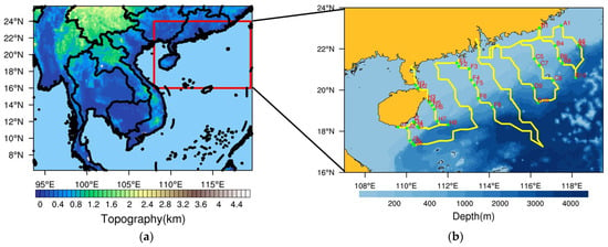
Figure 1.
The (a) WRF model simulation domain and topography map, contours with an interval 250 m represent the terrain height, and (b) the routes of scientific cruise represented by yellow lines. Green dots denote the locations of useable measurements derived from micro pulse lidar and red characters A-J indicate the cruising monitoring sites.

2.2.2. WRF Modeling Configuration
The WRF modeling system is a mesoscale non-hydrostatic numerical weather prediction system, which is designed to serve both operational forecasting and atmospheric research needs [32,33]. In this study, we conducted a WRF simulation for the scientific cruises in the SCS by using WRF version 4.0. The WRF simulation was run from 16 August 2016 00:00 UTC to 7 September 2016 00:00 UTC. The WRF model was set with one domain, shown in Figure 1a, using a 310 × 245 x-y grid of 9 km spacing, which covered most parts of the SCS, Southeast Asia, as well as part of the south China. The ERA5 reanalysis datasets provided by ECMWF, with a horizontal resolution of 0.25° (latitude) × 0.25° (longitude), vertical resolution of 38 levels, and a temporal resolution of 1 h, were used as initial and boundary conditions (ICBCs) to drive the WRF simulation. We tested many groups of parameterization schemes and selected the most suitable scheme for the study area (Table 1). In order to decrease the model uncertainties caused by long-term continuous integration, and thereby improve the simulation accuracy [34,35], data assimilation was turned on with the simulation nudged by ECMWF winds, temperature, and water vapor mixing ratio every 1 h throughout the whole atmospheric column in this study. The output from the WRF model was archived on an hourly basis. The initial 24 h were considered the spin-up period and, thus, were not used. Finally, the WRF simulation produced higher spatial resolution meteorological data provided with the Lagrangian simulation.

Table 1.
Model configuration and physical options of WRF model simulation.
2.2.3. FLEXPART-WRF Forward Simulations
FLEXPART-WRF was run forward with simulated emission from the mainland Southeast Asia for 72 h for each polluted measurement site in this study. Black carbon was selected as the tracer and released from 0 to 200 m above the ground level. Time series of hourly modelled concentrations were produced for polluted monitoring sites in the SCS. The vertical resolution of the FLEXPART-WRF output was the same as that of the extinction coefficient data. Sensitivity tests showed that the modelled episode start time at each of the measurement sites was independent of the start date of the simulations, provided sufficient lead time was given to allow transport from the mainland Southeast Asia to the northern SCS. The schedule of FLEXPART-WRF simulations is listed in Table 2. The emissions were set based on the MIX inventory for the year 2010. Wet and dry deposition during transportation was introduced in forward simulations.

Table 2.
The schedule of FLEXPART-WRF simulations.
2.2.4. Backward Trajectory Analysis for the Contribution of Anthropogenic PM2.5 to Non-Local Aerosols over the SCS
The output of FLEXPART-WRF in the backward trajectory simulation is residence time, also known as the “footprint” (unit: s). The residence time indicates the sensitivity of released particles at a receptor site to emissions from all grid cells in the simulation region. In this study, monitoring sites F2, F3, F4, and F6 of the scientific cruise were used as receptor sites in the backward trajectory simulations. We focused on anthropogenic emissions on the ground. The FLEXPART-WRF output for a thickness of 200 m (8 levels with an interval of 25 m, from 0 to 200 m) above the ground was considered as the “footprint”, and then used to calculate the contribution to the receptor site. The contribution from individual grid cells to the pollutant mass change at the receptor can be estimated by multiplying the residence time with air pollutant emission rates (unit: g s−1) in the respective grid cells [36,37,38].
Since most of the aerosols over the SCS concentrated on low-level (below 4 km) in this study [23], for each FLEXPART-WRF backward trajectory simulation, 300,000 particles were released in the first hour from 10 to 4000 m above ground level and followed backward in time for 72 h. The results were output with the residence time of particles in a horizontal resolution of 9 km × 9 km. A previous study showed that fine particulate matters dominated the aerosols transported into the SCS [9]. Therefore, the total residence time of particles over the 72 h backward trajectory at each grid point was multiplied by emission rates calculated from the MIX inventory to estimate the contribution of anthropogenic PM2.5 to non-local aerosols over the SCS. On the basis of these backward trajectory simulations, the main upwind potential sources of PM2.5 emissions for non-local aerosols at the receptors were identified using the contribution rate “contributionij”, calculated with Equation (1) [37,38].
where t is the time series of backward trajectory simulation period; the subscripts i = 1, …, N and j = 1, …, S denote the grid location (i, j) on the N × S grid of the simulation domain; Rijt denotes the time series residence time of backward simulation at (i, j); and Eij represents the PM2.5 emission rate at grid location (i, j).
3. Results
3.1. WRF Performance Evaluation
In this section, we performed a comprehensive evaluation of WRF simulation performance. The difference between the simulated mean value (Sim) and the observed mean value (Obs), or mean difference (Sim-Obs), between the simulations and observations, mean absolute error (MAE), root mean square error (RMSE), correlation coefficient (CC) and the hit rate (HR) were used to validate the simulation [39,40]. The MAE can accurately represent the actual prediction error, since it avoids an issue in which multiple predictions that have both positive and negative errors may compensate, leading to smaller than expected total error. The calculation formula of MAE is as follows:
The RMSE gives an overview of the accuracy of simulations, and the calculation formula of RMSE is as follows:
The CC indicates the strength and direction of a linear relationship between the simulation and observed values. The calculation formula of CC is as follows:
where S denotes the WRF simulations, O represents the observations, N is the quantity of grid points of verified region, and and represent mean simulated values and mean observational values, respectively.
The hourly 2 m relative humidity, 2 m air temperature, and surface winds from WRF were validated against observations from 20 meteorological stations (shown in Table 3). The simulated surface wind speed and the 2 m air temperature were slightly biased high, with mean differences of 0.91 m s−1 and 0.1 °C, respectively. The simulated 2 m relative humidity was slightly biased low, with a mean difference of 2.4%. The CC of 2 m relative humidity and the 2 m air temperature were 0.76 and 0.84, respectively, indicating good agreement between the simulation and observations. However, the CC of wind direction and wind speed were 0.31 and 0.62, respectively, indicating that the simulated 10 m surface winds did not match well with observations.

Table 3.
The statistical results of simulated data and hourly observed meteorological data.
The HR is defined as a fraction of the total simulation records that are within a certain observation threshold. It is a reliable evaluation method of model performance since it accounts for observation uncertainty, an issue that is difficult to consider using the mean difference, the CC, or the RMSE. The standard for a “hit” requires that the difference between observations and simulations fall within 2 °C for 2 m air temperature, 10% for 2 m relative humidity, 30° for surface wind direction, and 1 m s−1 for surface wind speed [40,41]. The HR of the 2 m air temperature, 2 m relative humidity, surface wind speed, and surface wind direction, calculated using these thresholds, were 0.87, 0.68, 0.50, and 0.42, respectively. This indicated that simulated 2 m air temperature, 2 m relative humidity and surface winds speed were realistic. The HR of surface wind direction was lower than that of the other variables. However, the above statistics were well within reasonable ranges compared with previous studies on short-term dynamical downscaling, and some were slightly better [41,42,43]. This indicated that the simulation reasonably matched observations during the study period.
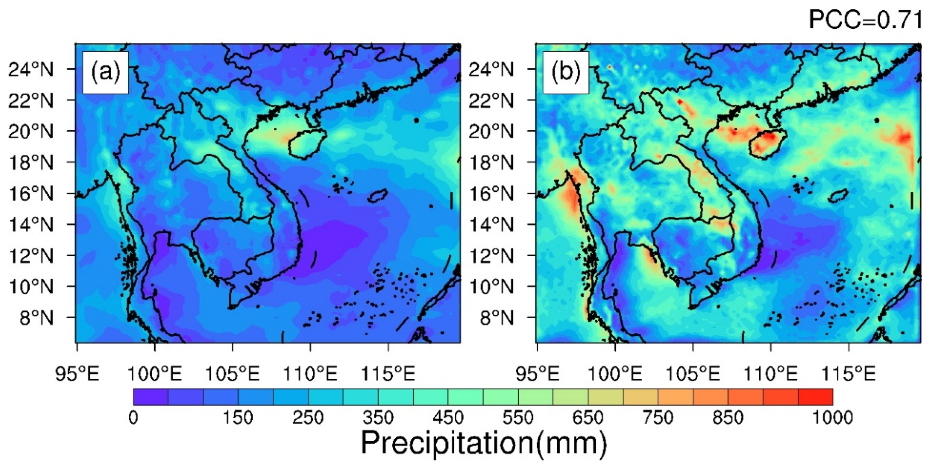
FLEXPART includes tracer attenuation through dry and wet deposition [44]. Since wet deposition can be significant, the accuracy of WRF precipitation is also important for the FLEXPART simulation. We further verified hourly total precipitation from WRF against the ERA5 reanalysis. To facilitate comparisons, the WRF output was interpolated to the ERA5 grid, from the horizontal resolution of 9 km × 9 km to 0.25° × 0.25°. The distributions of accumulated precipitation from ERA5 and WRF are displayed in Figure 2. The hourly total precipitation of WRF and ERA5 showed a common feature in that the rain belt in both ERA5 and WRF was mainly located in the northern SCS, while less precipitation fell in the southern SCS. The major precipitation centers were located in the Beibu Gulf, the eastern coast of Myanmar, and central Laos. As a whole, WRF was able to effectively capture the location of maximum and minimum of precipitation. The spatial correlation coefficient between WRF and ERA5 was 0.71, indicating that WRF reproduced the spatial distribution of the rain belt. However, the hourly total precipitation from WRF was higher than ERA5. Since most tropical monsoon precipitation is convective, this suggested that the Kain-Fritsch cumulus parameterization scheme produced more cumulus precipitation than realistic during the scientific cruise period. In addition, since nudging analysis was used throughout the whole atmospheric column in the WRF simulation, the surface variable might have been nudged towards unrealistic values, resulting in biased precipitation [45,46].

Figure 2.
Distribution of total precipitation from 17 August 2016 to 6 September 2016. (a) ERA5, and (b) WRF simulations.
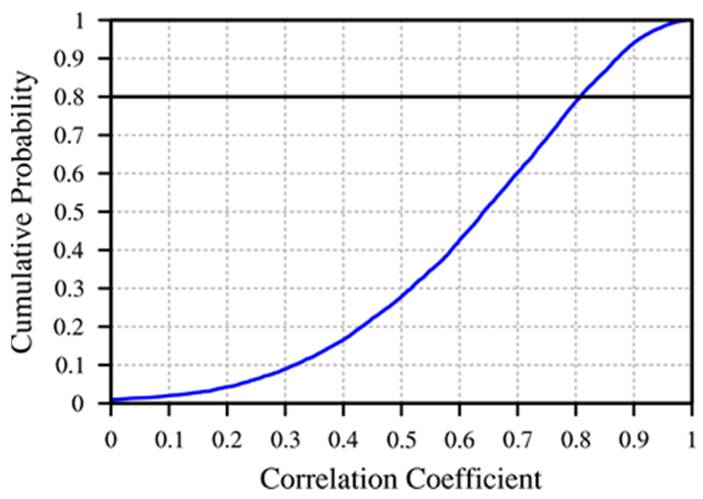
The accuracy of the simulated precipitation at each grid point was determined by the correlation coefficients between times series of 24 h accumulated precipitation of the WRF and ERA5 total daily precipitation (Figure 3), during the period of 17 August 2016 to 6 September 2016. The correlation coefficients, shown in Figure 3, give a spatial indication of the model performance. The correlation coefficients were more than 0.6 in most of the oceanic regions. However, the correlation coefficients were less than 0.4 over most of the terrestrial regions, especially over the south of terrestrial Southeast Asia. Hence, precipitation was less well simulated over land than over the ocean. The cumulative distribution of grid-point correlation coefficients is shown in Figure 4. The vertical axis gives the percentage of grid-points in the domain that have correlation coefficients (CC) less than or equal to the value given in the horizontal axis. From Figure 4, WRF performed very well (CC > 0.8) over 21% of the verification region, and performed poorly (CC ≤ 0.4) over 17% of the verification region. Performance was intermediate (0.4 < CC ≤ 0.8) over the remaining 62% of the verification region. The downscaling of precipitation in regional climate models is difficult, especially precipitation over monsoon regions. To improve the dynamical downscaling performance in these regions, advances in the dynamic solver of the WRF model and parameterized physics are required [45]. In summary, we estimated the WRF performance in simulating precipitation, and found that the WRF model could reproduce the basic temporal and spatial variations of precipitation in the verification area.
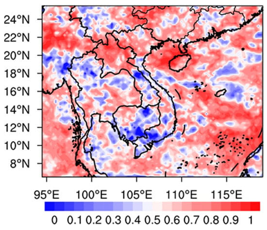
Figure 3.
The correlation coefficients between time series of total daily precipitation of WRF simulations and ERA5 reanalysis data at each grid point from 17 August 2016 to 6 September 2016.
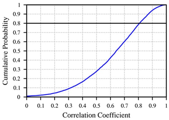
Figure 4.
The cumulative probability of distribution of grid-point correlation coefficients shown in Figure 3 from 17 August 2016 to 6 September 2016.
3.2. FLEXPART-WRF Evaluation
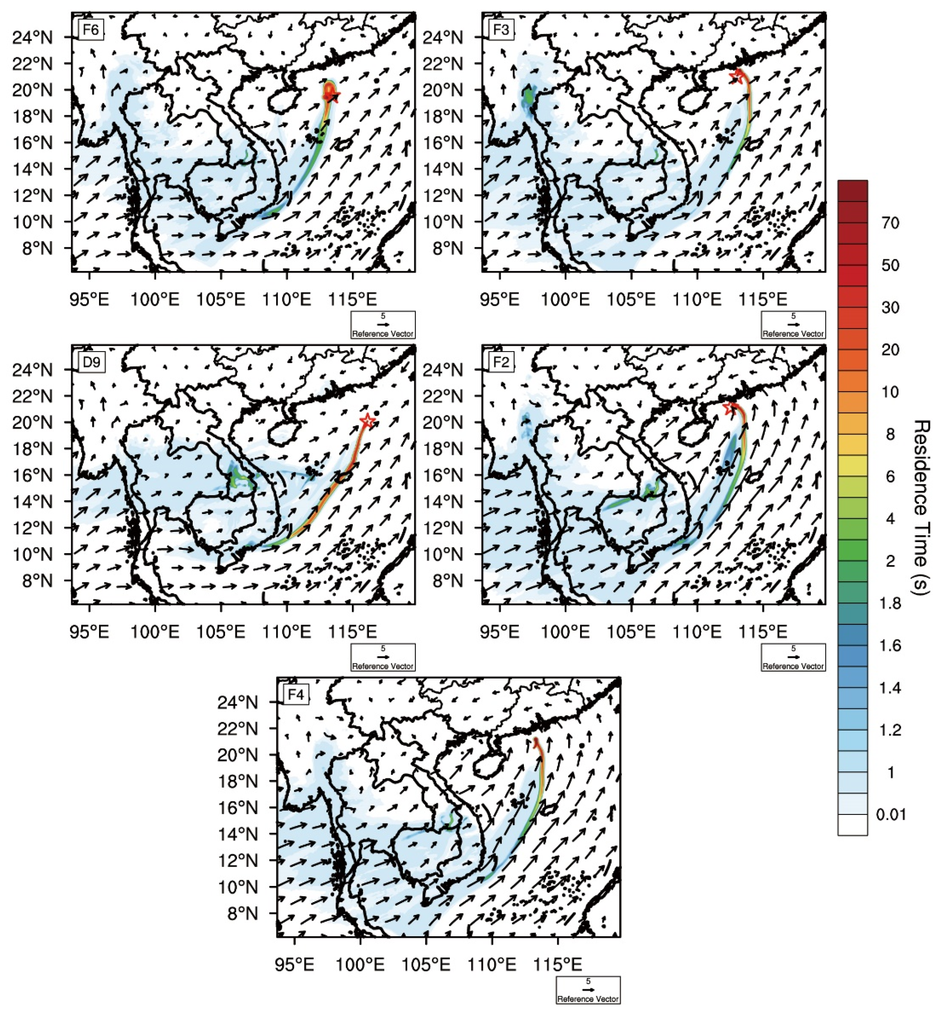
The vertical distributions of aerosols over the SCS was modeled using FLEXPART-WRF forward simulations and compared with aerosol extinction coefficients calculated from lidar measurements on the scientific cruise. This study focused on the areas surrounding routes D- and F- of the scientific cruise. Since measurements at each monitoring site were taken at different times, the emission sources affecting these monitoring sites might be significantly different. We first conducted backward trajectory simulations to determine the sources which might potentially affect each monitoring site within 72 h, and to reduce errors caused by emission sources settings in forward simulations. The backward trajectory simulations showed that aerosols over route D- and route F- were mainly transported from mainland Southeast Asia by southwesterly prevailing winds in the middle- and low-level atmosphere (as shown in Figure 5). Since there was little biomass burning in mainland Southeast Asia during the cruise period (as shown in Figure 6), we only considered the effect of anthropogenic emission from mainland Southeast Asia on the distribution of aerosols over the SCS. On the basis of the results of these backward trajectory simulations, and using the Asian anthropogenic emission inventory of 2010, we set up a series of continuously releasing pollution sources in mainland Southeast Asia and then conducted 72 h forward simulations for each of the polluted monitoring sites. To facilitate the comparison between the FLEXPART-WRF output and the lidar-derived extinction coefficients, the FLEXPART-WRF output was interpolated onto the monitoring sites F2, F3, F4, F6, and D9.
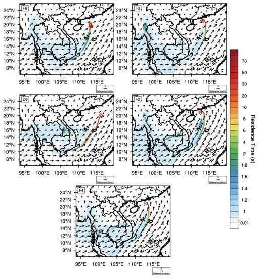
Figure 5.
The spatial distribution of residence time (in units of s) of 72 h backward trajectory simulations at monitoring sites F2, F3, F4, F6, and D9. The vector arrow is 72 h surface wind field (in units of m s−1). The red stars denote the position of monitoring sites (receptors).
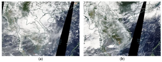
Figure 6.
Satellite imagery for biomass burning, obtained from the NASA Worldview application (http://worldview.earthdata.nasa.gov/ (accessed on 20 November 2020)), and fire spots from Terra over (a) 17 August 2016 to 20 August 2016 (left); and (b) 2 September 2016 to 5 September 2016 (right).
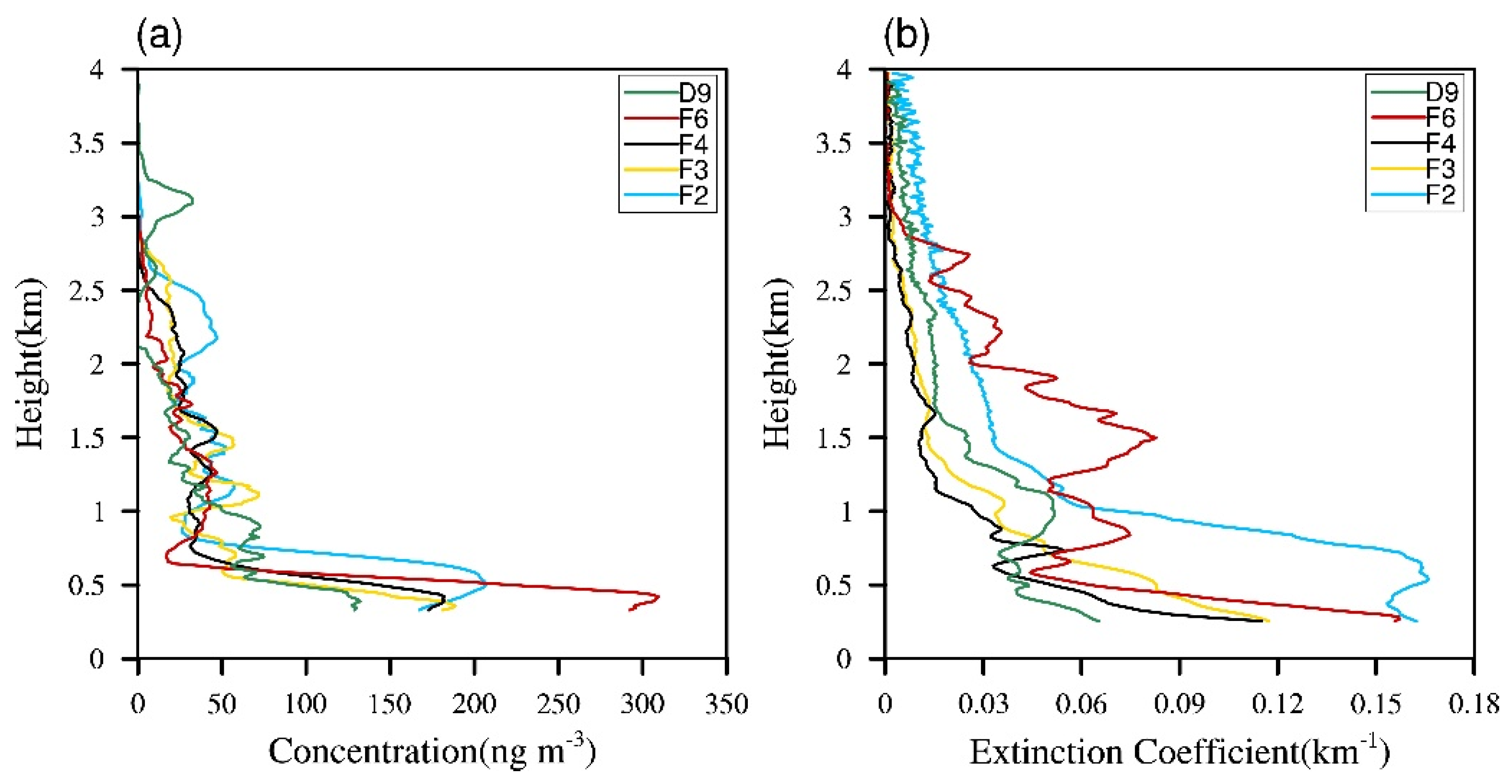
The vertical profiles of BC concentration simulated by the FLEXPART-WRF model and the vertical profiles of the aerosol extinction coefficient at monitoring sites F2, F3, F4, F6, and D9 are displayed in Figure 7. The results showed that the simulated BC concentration over the South China Sea was slightly lower than the findings of Yin et al. (2019) [47]. The lidar-derived extinction coefficients were 0.060–0.165 km−1 below 1 km, and very close to 0 above 3.5 km (Figure 7b). This suggested that aerosols were mainly concentrated below 1 km and did not diffuse to above 3.5 km. Such vertical distributions were produced by the FLEXPART-WRF (Figure 7a). The extinction coefficient between 0.5 km and 0.7 km was larger at F2 than that at other monitoring sites, and the FLEXPART-WRF produced higher BC concentrations than at other monitoring sites. The vertical distribution of aerosols at F2 was reproduced by the FLEXPART-WRF model.
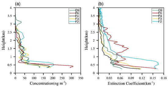
Figure 7.
The (a) vertical profiles of BC concentration simulated by FLEXPART-WRF at monitoring sites F2, F3, F4, F6, and D9; and the (b) vertical profiles of the extinction coefficient at monitoring sites F2, F3, F4, F6, and D9.
We quantitatively verified the performance of the FLEXPART-WRF model using the correlation coefficient between the vertical concentration profile and extinction coefficient profile at each monitoring site, as shown in Table 4. The correlation coefficients at monitoring sites F2, F3, F4, F6, and D9 were 0.88, 0.90, 0.88, 0.70, and 0.82, respectively. This suggested that the vertical distribution of the aerosols was reproduced by the model. The vertical profiles of extinction coefficient were measured at specific times, while the results of the FLEXPART-WRF model reflected the time-mean transport of aerosols over different conditions of atmospheric circulation. Some discrepancies would be expected. In the forward simulation, we only released one species and used it to evaluate the ability of the FLEXPART-WRF to simulate the particle transport, which might cause the deviation of the vertical distribution of particles. For example, the extinction coefficient curve at measurement site F6 presented a bimodal structure with a peak value of more than 0.07 km−1, but this feature was not reproduced by the model.

Table 4.
Correlation coefficient between vertical concentration profile and extinction coefficient profile at monitoring sites F2, F3, F4, F6, and D9.
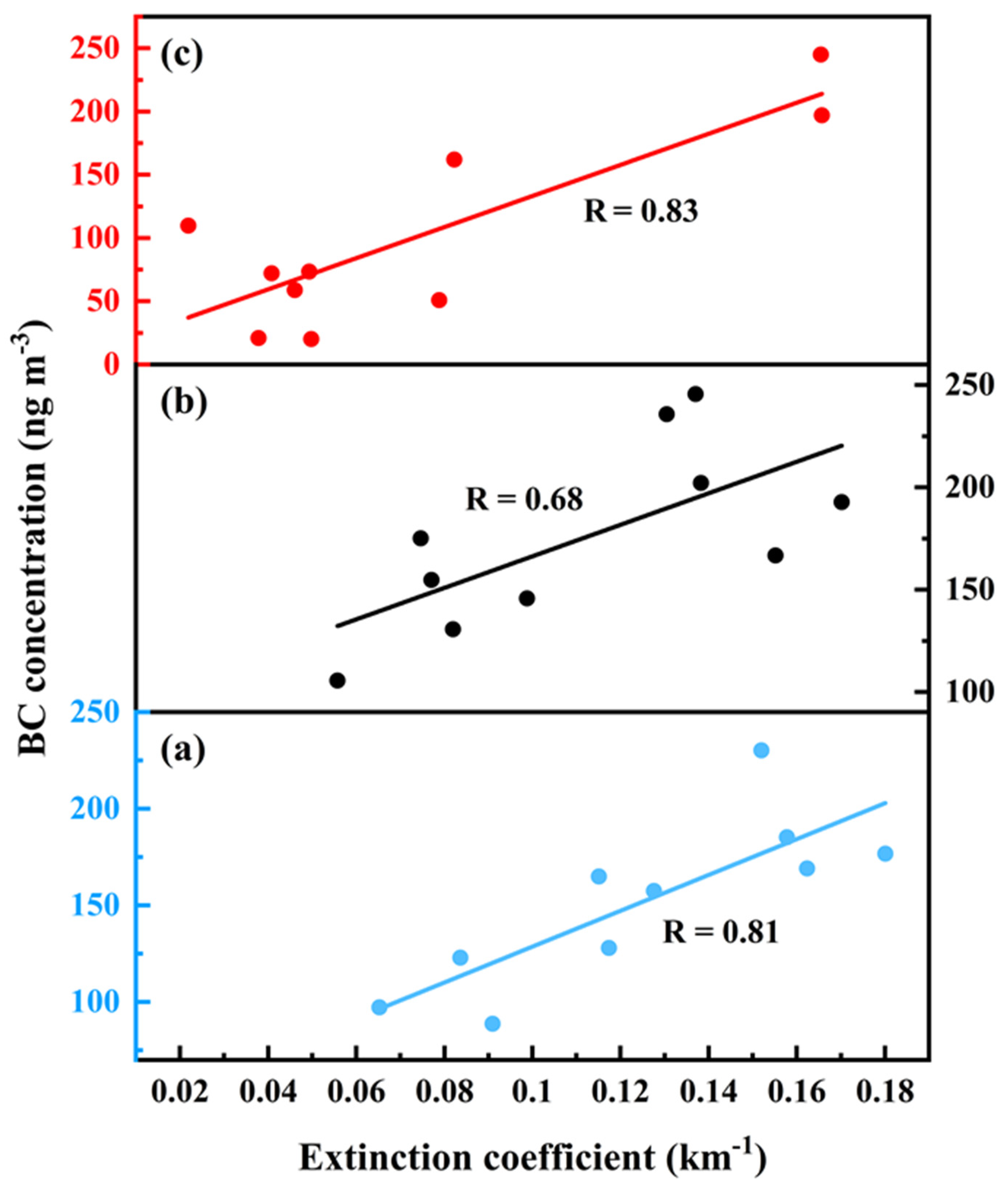
We compared the simulated concentration within the planetary boundary layer with the measured extinction coefficient. Powell et al. (2000) measured the marine aerosol extinction using a micro pulse lidar and obtained an aerosol extinction coefficient ranging from 0.02 to 0.07 km−1 for unpolluted conditions [48]. Based on the result of Powell et al., we considered measurement sites with a maximum extinction coefficient of more than 0.07 km−1 as polluted measurement sites. Li et al. found the mean planetary boundary layer height (PBLH) was 653.2 m during the scientific cruise. It was noted that the vertical range of the micro pulse lidar system on the ship was from 250 m to 4000 m [23]. We selected the polluted measurement sites to calculate the correlation coefficient between the simulated concentration and the observed extinction coefficient at three different layers within the planetary boundary layer. The linear correlation between BC concentration and extinction coefficient at 250 m, 350 m, and 550 m are shown in Figure 8. Overall, the correlations at 250 m, 350 m, and 550 m were 0.81, 0.68, and 0.83, respectively. This suggested that the vertical distribution of the aerosols was also reproduced by the model.
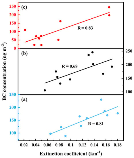
Figure 8.
The linear correlation between BC concentration and extinction coefficient at three different layers, with correlation coefficients (R) shown in the figure. (a) 250 m, (b) 350 m, and (c) 550 m.
3.3. Contribution of Anthropogenic PM2.5 to Non-Local Aerosols over the SCS
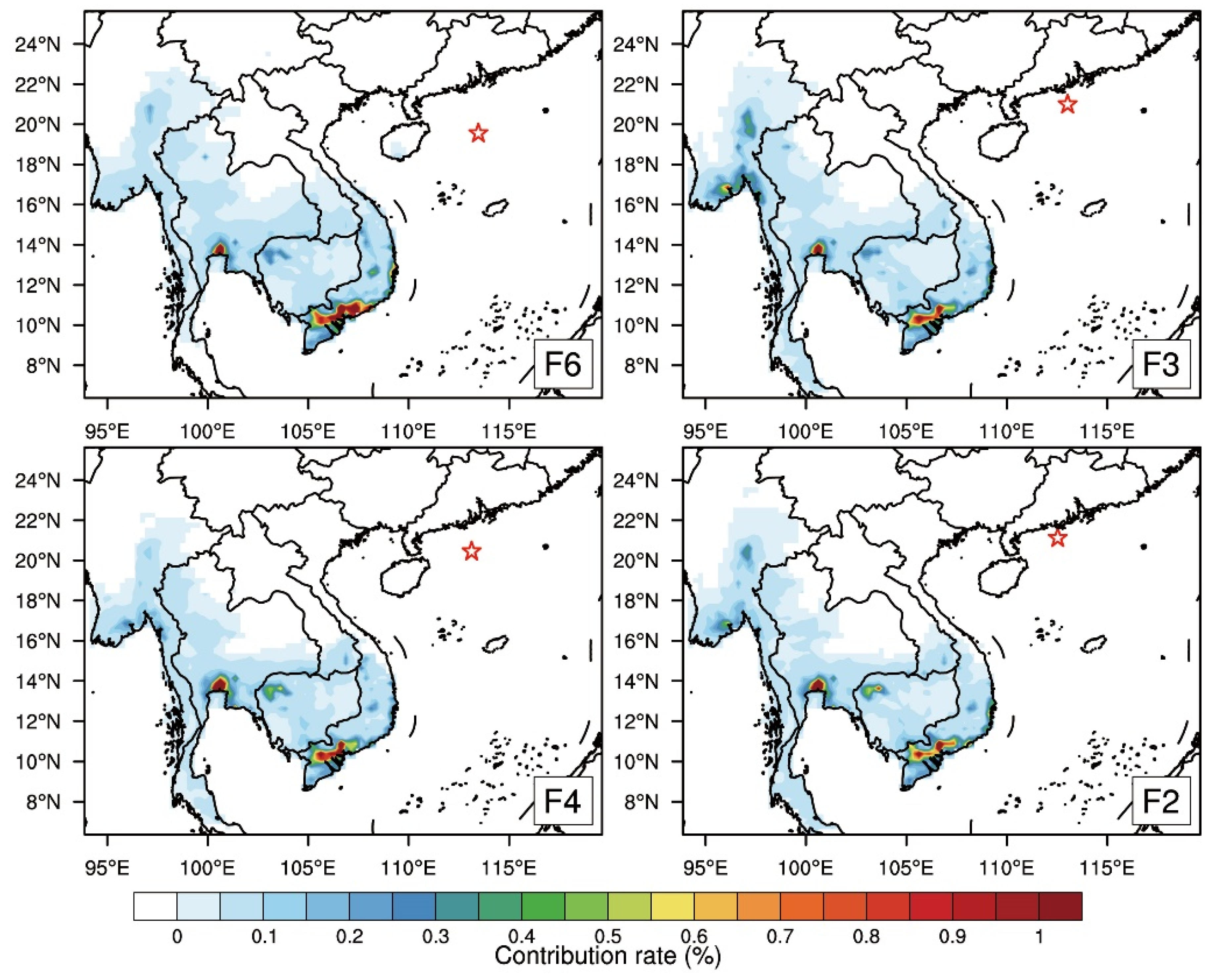
We selected four polluted measurement sites and estimated the regional contributions to observed pollution over the SCS. The contribution rates of non-local sources were calculated with Equation (1), shown in Figure 9. The model result showed that sources in mainland Southeast Asia contributed to more than 90% of the non-local aerosols at the three monitoring sites. This was because the prevailing winds were southwesterly during the scientific cruise. The major pathways of transport were a southern route from Ho Chi Minh City, Vietnam, a mid-route from Bangkok, Thailand, and a northern route from the southern coastal areas of Myanmar. Transport from the source regions in Ho Chi Minh City and Bangkok regions contributed significantly to the non-local aerosols at monitoring sites F2, F3, F4, and F6.
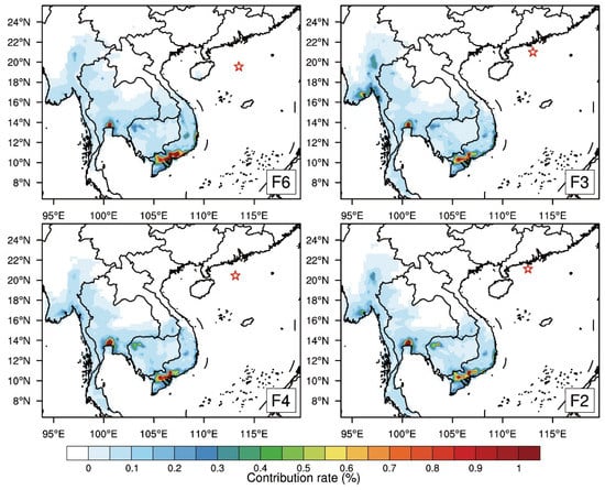
Figure 9.
Spatial distribution of contribution rate of regional transport (color contours) to non-local aerosols at monitoring sites F2, F3, F4, and F6 simulated by the FLEXPART-WRF model. Red stars denote the location of monitoring sites.
We further investigated the contributions of individual countries in mainland Southeast Asia to non-local aerosols at monitoring sites F2, F3, F4, and F6. As shown in Table 5, Vietnam and Thailand were the main contributors, with mean contribution rates of 39.6% and 25.1%, respectively. Although the mean contribution rate of Myanmar was lower at 16.7%, it was still a significant pollution source since its contribution rate at monitoring site F3 was second to Vietnam at 26.5%. The mean contribution rates of Laos and Cambodia were minor at 1.86% and 10.3%, respectively.

Table 5.
The potential contributions of individual countries in mainland Southeast Asia to four receptors, F2, F3, F4, and F6. (unit: %).
Typically, scientists or researchers use Eulerian models with the ability to describe complex non-linear chemistry process, such as WRF-Chem and GEOS-Chem, to quantitatively estimate the contribution of regional transport to air pollution [32,49,50]. In this study, we applied the Lagrangian particle dispersion model (LPDM) FLEXPART-WRF to calculate the contribution rates of anthropogenic PM2.5 to non-local aerosols over the SCS. The main uncertainty of the Lagrange method for such calculations, as compared to Eulerian methods, is that this method ignores the complex non-linear chemistry reaction, which is crucial to the formation of secondary aerosols. This uncertainty may underestimate the contribution of source regions to receptors. Many previous studies, however, have shown that using this method to quantity the contribution of regional transport to air pollution is feasible [37,38].
4. Discussions and Conclusions
The major purpose of this study was to evaluate the applicability of FLEXPART-WRF as an air pollution forecasting system and to estimate the contribution of anthropogenic PM2.5 to non-local aerosols over the SCS. The model was verified against meteorological observations collected at 20 stations and aerosol extinction coefficients measured by shipborne micro pulse lidar in the SCS. The simulated 2 m air temperature and surface wind speed were slightly greater than observed, with mean differences of 0.1 °C and 0.91 m s−1, respectively. The simulated 2 m relative humidity was slightly less than observed, with a mean difference of 2.4%. The correlation coefficients of 2 m air temperature, 2 m relative humidity, surface wind speed and direction were 0.84, 0.76, 0.62, and 0.31, respectively, indicating that the WRF model reproduced the meteorological elements.
The simulated wind direction was within reasonable ranges compared with previous studies [41,43,51,52]. There were few coupled climate models that could reproduce surface wind direction with better accuracy. Despite the fact that using finer land use and surface textures in the model can improve the simulated elements, the surface wind is influenced by many complicated physical processes (e.g. turbulence processes, thermal effect, and topography) and is usually characterized by a considerable sub-grid scale in the model.
FLEXPART-WRF simulated the vertical distribution of aerosols over the northern SCS. The concentration, however, was slightly lower than a previous study [47]. The low concentration was likely induced by an overestimation of the precipitation, resulting in excessive removal processes. In addition, the non-linear chemical reactions were not involved, which was crucial to the formation of secondary aerosols and may have been another factor for biases.
Many previous studies found that pollutants transported into the SCS mainly originate from eastern China. However, our results showed that the non-local aerosols over the northern SCS were mainly from Southeast Asia, which indicated that emissions from Southeast Asia also had an important impact.
The model results showed that sources in mainland Southeast Asia contributed to more than 90% of non-local aerosols along the cruise path. This was explained by the strong southwesterly monsoon winds. Vietnam and Thailand were the main sources of PM2.5, accounting for 39.6% and 25.1%, respectively. Burning aerosols have a large short-term impact on the pollutant concentration. It will be helpful to track such sources and update emission inputs using near real-time monitoring methods [53,54,55,56]. Further modelling of physical processes and the improvement of the model resolution are also expected to improve the performance.
Author Contributions
Y.T.: software, validation, formal analysis, writing—original draft, and visualization. Z.J.: conceptualization, methodology, investigation, writing—review and editing, and supervision. Y.L.: software, and data curation. Z.H.: validation, writing—original draft. X.Z.: resources and formal analysis. W.D.: supervision and project administration. All authors have read and agreed to the published version of the manuscript.
Funding
This research was funded by the Second Tibetan Plateau Scientific Expedition and Research Program (2019QZKK0605), the National Key Research and Development Program of China (2016YFA0602701), Innovation Group Project of Southern Marine Science and Engineering Guangdong Laboratory (Zhuhai) (No. 311020008), and the Open Program (SKLCS-OP-2020-9) from the State Key Laboratory of Cryospheric Science, Northwest Institute of Eco-Environment and Resources, Chinese Academy of Sciences.
Institutional Review Board Statement
Not applicable.
Informed Consent Statement
Not applicable.
Data Availability Statement
The observational meteorological data can be download in the Meteorological Data Sharing Network of the China Meteorological Administration (http://data.cma.cn). The emission inventory is provided by the Department of Earth System Science Tsinghua University (http://www.meicmodel.org). The lidar data are available on request from the corresponding author.
Acknowledgments
We thank Shao-yi Lee for re-editing the English written. Three anonymous reviewers’ suggestion and academical editor’s comment were kindly appreciated.
Conflicts of Interest
The authors declare no conflict of interest.
References
- Haywood, J.; Boucher, O. Estimates of the direct and indirect radiative forcing due to tropospheric aerosols: A review. Rev. Geophys. 2000, 38, 513–543. [Google Scholar] [CrossRef]
- Jia, R.; Liu, Y.; Chen, B.; Zhang, Z.; Huang, J. Source and transportation of summer dust over the Tibetan Plateau. Atmos. Environ. 2015, 123, 210–219. [Google Scholar] [CrossRef]
- Levy, H.; Horowitz, L.W.; Schwarzkopf, M.D.; Ming, Y.; Golaz, J.C.; Naik, V.; Ramaswamy, V. The roles of aerosol direct and indirect effects in past and future climate change. J. Geophys. Res. Atmos. 2013, 118, 4521–4532. [Google Scholar] [CrossRef]
- Quaas, J.; Boucher, O.; Bellouin, N.; Kinne, S. Satellite-based estimate of the direct and indirect aerosol climate forcing. J. Geophys. Res. Atmos. 2008, 113, D5. [Google Scholar] [CrossRef]
- Kaufman, Y.J.; Tanré, D.; Gordon, H.R.; Nakajima, T.; Lenoble, J.; Frouin, R.; Grassl, H.; Herman, B.M.; King, M.D.; Teillet, P.M. Passive remote sensing of tropospheric aerosol and atmospheric correction for the aerosol effect. J. Geophys. Res. Atmos. 1997, 102, 16815–16830. [Google Scholar] [CrossRef] [Green Version]
- Bréon, F.M.; Tanré, D.; Generoso, S. Aerosol effect on cloud droplet size monitored from satellite. Science 2002, 295, 834–838. [Google Scholar] [CrossRef] [PubMed]
- Tseng, C.; Wong, G.T.; Lin, I.; Wu, C.; Liu, K. A unique seasonal pattern in phytoplankton biomass in low-latitude waters in the South China Sea. Geophys. Res. Lett. 2005, 32, L08608. [Google Scholar] [CrossRef] [Green Version]
- Sheu, G.R.; Lin, N.H.; Lee, C.T.; Wang, J.L.; Chuang, M.T.; Wang, S.H.; Kai, H.C.; Ou-Yang, C.F. Distribution of atmospheric mercury in northern Southeast Asia and South China Sea during Dongsha Experiment. Atmos. Environ. 2013, 78, 174–183. [Google Scholar] [CrossRef]
- Lin, I.I.; Chen, J.P.; Wong, G.T.F.; Huang, C.W.; Lien, C.C. Aerosol input to the South China Sea: Results from the MODerate Resolution Imaging Spectro-radiometer, the Quick Scatterometer, and the Measurements of Pollution in the Troposphere Sensor. Deep Sea Res. Top. Stud. Oceanogr. 2007, 54, 1589–1601. [Google Scholar] [CrossRef]
- Zhang, C.; Xu, H.; Li, Z.; Xie, Y.; Li, D. Maritime Aerosol Optical and Microphysical Properties in the South China Sea Under Multi-source Influence. Sci. Rep. 2019, 9, 17796. [Google Scholar] [CrossRef]
- Tan, H.; Wu, D.; Bi, X. Measurement and study of aerosol optical depth over northern South China Sea. J. Tropical. Oceanogr. 2006, 25, 21–25. [Google Scholar]
- Zhang, X.; Zhuang, G.; Guo, J.; Yin, K.; Zhang, P. Characterization of aerosol over the northern South China Sea during two cruises in 2003. Atmos. Environ. 2007, 41, 7821–7836. [Google Scholar] [CrossRef]
- Chester, R.; Bradshaw, G.F.; Corcoran, P.A. Trace metal chemistry of the North Sea particulate aerosol: Concentrations, source and sea water fates. Atmos. Environ. 1994, 28, 2873–2883. [Google Scholar] [CrossRef]
- Reid, J.S.; Hyer, E.J.; Johnson, R.S.; Holben, B.N.; Yokelson, R.J.; Zhang, J.; Campbell, J.R.; Christopher, S.A.; di Girolamo, L.; Giglio, L.; et al. Observing and understanding the Southeast Asian aerosol system by remote sensing: An initial review and analysis for the Seven Southeast Asian Studies (7SEAS) program. Atmos. Res. 2013, 122, 403–469. [Google Scholar] [CrossRef] [Green Version]
- Srinivas, C.V.; Rajagopal, V.; Baskaran, R.; Vinay, R.; Venkatraman, B. Regional scale atmospheric dispersion simulation of accidental releases of radionuclides from Fukushima Dai-ichi reactor. Atmos. Environ. 2012, 61, 66–84. [Google Scholar] [CrossRef]
- Madala, S.; Prasad, K.H.; Srinivas, C.V.; Satyanarayana, A.N.V. Air quality simulation of NOX over the tropical coastal city Chennai in southern India with FLEXPART-WRF. Atmos. Environ. 2016, 128, 65–81. [Google Scholar] [CrossRef]
- Palau, J.L.; Pérez-Landa, G.; Meliá, J.; Segarra, D.; Millán, M.M. A study of dispersion in complex terrain under winter conditions using high-resolution mesoscale and Lagrangian particle models. Atmos. Chem. Phys. 2005, 6, 1105–1134. [Google Scholar] [CrossRef] [Green Version]
- Cécé, R.; Bernard, D.; Brioude, J.; Zahibo, N. Microscale anthropogenic pollution modelling in a small tropical island during weak trade winds: Lagrangian particle dispersion simulations using real nested LES meteorological fields. Atmos. Environ. 2016, 139, 98–112. [Google Scholar] [CrossRef]
- Zhu, Q.; Liu, Y.; Jia, R.; Hua, S.; Shao, T.; Wang, B. A numerical simulation study on the impact of smoke aerosols from Russian forest fires on the air pollution over Asia. Atmos. Environ. 2018, 182, 263–274. [Google Scholar] [CrossRef]
- Solomos, S.; Amiridis, V.; Zanis, P.; Gerasopoulos, E.; Sofiou, F.I.; Herekakis, T.; Brioude, J.; Stohl, A.; Kahn, R.A.; Kontoes, C. Smoke dispersion modeling over complex terrain using high resolution meteorological data and satellite observations—The FireHub platform. Atmos. Environ. 2015, 119, 348–361. [Google Scholar] [CrossRef]
- Brioude, J.; Arnold, D.; Stohl, A.; Cassiani, M.; Morton, D.; Seibert, P. The Lagrangian particle dispersion model FLEXPART-WRF version 3.1. Geosci. Model Dev. 2013, 6, 1889–1904. [Google Scholar] [CrossRef] [Green Version]
- Arnold, D.; Maurer, C.; Wotawa, G.; Draxler, R.; Saito, K.; Seibert, P. Influence of the meteorological input on the atmospheric transport modelling with FLEXPART of radionuclides from the Fukushima Daiichi nuclear accident. J. Environ. Radioact. 2015, 139, 212–225. [Google Scholar] [CrossRef]
- Li, Y.; Wang, B.; Lee, S.-Y.; Zhang, Z.; Wang, Y.; Dong, W. Micro-Pulse Lidar Cruising Measurements in Northern South China Sea. Remote Sens. 2020, 12, 1695. [Google Scholar] [CrossRef]
- Li, M.; Zhang, Q.; Kurokawa, J.-I.; Woo, J.-H.; He, K.; Lu, Z.; Ohara, T.; Song, Y.; Streets, D.G.; Carmichael, G.R. MIX: A mosaic Asian anthropogenic emission inventory under the international collaboration framework of the MICS-Asia and HTAP. Atmos. Chem. Phys. 2017, 17, 935–963. [Google Scholar] [CrossRef] [Green Version]
- Stohl, A.; Forster, C.; Frank, A.; Seibert, P.; Wotawa, G. Technical note: The Lagrangian particle dispersion model FLEXPART version 6.2. Atmos. Chem. Phys. 2005, 5, 2461–2474. [Google Scholar] [CrossRef] [Green Version]
- Pisso, I.; Sollum, E.; Grythe, H.; Kristiansen, N.I.; Cassiani, M.; Eckhardt, S.; Arnold, D.; Morton, D.; Thompson, R.L.; Groot Zwaaftink, C.D.; et al. The Lagrangian particle dispersion model FLEXPART version 10.4. Geosci. Model Dev. 2019, 12, 4955–4997. [Google Scholar] [CrossRef] [Green Version]
- Seibert, P.; Frank, A. Source-receptor matrix calculation with a Lagrangian particle dispersion model in backward mode. Atmos. Chem. Phys. 2004, 4, 51–63. [Google Scholar] [CrossRef] [Green Version]
- Fast, J.D.; Easter, R.C. A Lagrangian particle dispersion model compatible with WRF. In Proceedings of the 7th WRF Users Workshop, Boulder, CO, USA, 19–22 June 2006; pp. 19–22. [Google Scholar]
- Angevine, W.M.; Brioude, J.; McKeen, S.; Holloway, J.S. Uncertainty in Lagrangian pollutant transport simulations due to meteorological uncertainty from a mesoscale WRF ensemble. Geosci. Model Dev. 2014, 7, 2817–2829. [Google Scholar] [CrossRef] [Green Version]
- de Foy, B.; Varela, J.R.; Molina, L.T.; Molina, M.J. Rapid ventilation of the Mexico City basin and regional fate of the urban plume. Atmos. Chem. Phys. 2006, 6, 2321–2335. [Google Scholar] [CrossRef] [Green Version]
- Angevine, W.M.; Brioude, J.; Mckeen, S.; Holloway, J.S.; Lerner, B.M.; Goldstein, A.H.; Guha, A.; Andrews, A.; Nowak, J.B.; Evan, S. Pollutant transport among California regions. J. Geophys. Res. Atmos. 2013, 118, 6750–6763. [Google Scholar] [CrossRef]
- Skamarock, W.C.; Klemp, J.B.; Dudhia, J.; Gill, D.O.; Barker, D.M.; Duda, M.G.; Huang, X.-Y.; Wang, W.; Powers, J.G. A Description of the Advanced Research WRF Version 3; NCAR Technical Report; NCAR: Boulder, CO, USA, 2008. [Google Scholar]
- Liu, Y.; Hong, Y.; Fan, Q.; Wang, X.; Chan, P.W.; Chen, X.; Lai, A.; Wang, M.; Chen, X. Source-receptor relationships for PM 2.5 during typical pollution episodes in the Pearl River Delta city cluster, China. Sci. Total Environ. 2017, 596, 194–206. [Google Scholar] [CrossRef]
- Glisan, J.; Gutowski, W.; Cassano, J.; Higgins, M. Effects of Spectral Nudging in WRF on Arctic Temperature and Precipitation Simulations. J. Clim. 2013, 26, 3985–3999. [Google Scholar] [CrossRef]
- Bullock, O.R.; Alapaty, K.; Herwehe, J.A.; Mallard, M.S.; Nolte, C.G. An observation-based investigation of nudging in WRF for downscaling surface climate information to 12-km grid spacing. J. Appl. Meteorol. Climatol. 2013, 53, 20–33. [Google Scholar] [CrossRef]
- Stohl, A.; Forster, C.; Eckhardt, S.; Huntrieser, H.; Heland, J.; Schlager, H.; Aufmhoff, H.; Arnold, F.; Cooper, O. A backward modeling study of intercontinental pollution transport using aircraft measurements. J. Geophys. Res. Atmos. 2003, 108, D12. [Google Scholar] [CrossRef]
- Ding, A.; Tao, W.; Xue, L.; Gao, J.; Stohl, A.; Lei, H.; Jin, D.; Ren, Y.; Wang, X.; Wei, X. Transport of north China air pollution by midlatitude cyclones: Case study of aircraft measurements in summer 2007. J. Geophys. Res. Atmos. 2009, 114, D08304. [Google Scholar] [CrossRef] [Green Version]
- Yu, C.; Zhao, T.; Bai, Y.; Zhang, L.; Kong, S.; Yu, X.; He, J.; Cui, C.; Yang, J.; You, Y. Heavy air pollution with a unique “non-stagnant” atmospheric boundary layer in the Yangtze River middle basin aggravated by regional transport of PM2.5 over China. Atmos. Chem. Phys. 2020, 20, 7217–7230. [Google Scholar] [CrossRef]
- Fan, Q.; Liu, Y.M.; Wang, X.M.; Fan, S.J.; Chan, P.W.; Lan, J.; Feng, Y.R. Effect of different meteorological fields on the regional air quality modelling over Pearl River Delta, China. Int. J. Environ. Pollut. 2013, 53, 3–23. [Google Scholar] [CrossRef]
- Schlünzen, K.H.; Katzfey, J.J. Relevance of sub-grid-scale land-use effects for mesoscale model. Tellus Dyn. Meteorol. Oceanogr. 2003, 55, 232–246. [Google Scholar] [CrossRef]
- Jiang, F.; Guo, H.; Wang, T.; Cheng, H.; Wang, X.; Simpson, I.; Ding, A.; Saunders, S.M.; Lam, S.; Blake, D.R. An ozone episode in the Pearl River Delta: Field observation and model simulation. J. Geophys. Res. Atmos. 2010, 115, 1–18. [Google Scholar] [CrossRef]
- Wang, X.M.; Liu, H.; Pang, J.M.; Carmichael, G.; He, K.B.; Fan, Q.; Zhong, L.J.; Wu, Z.Y.; Zhang, J.P. Reductions in sulfur pollution in the Pearl River Delta region, China: Assessing the effectiveness of emission controls. Atmos. Environ. 2013, 76, 113–124. [Google Scholar] [CrossRef]
- Wang, N.; Guo, H.; Jiang, F.; Ling, Z.H.; Wang, T. Simulation of ozone formation at different elevations in mountainous area of Hong Kong using WRF-CMAQ model. Sci. Total Environ. 2015, 505, 939–951. [Google Scholar] [CrossRef]
- An, X.; Yao, B.; Li, Y.; Li, N.; Zhou, L. Tracking source area of Shangdianzi station using Lagrangian particle dispersion model of FLEXPART. Meteorol. Appl. 2014, 21, 466–473. [Google Scholar] [CrossRef]
- Lo, J.C.F.; Yang, Z.L.; Pielke Sr, R.A. Assessment of three dynamical climate downscaling methods using the Weather Research and Forecasting (WRF) model. J. Geophys. Res. Atmos. 2008, 113, D09112. [Google Scholar] [CrossRef]
- Pohl, B.; Crétat, J. On the use of nudging techniques for regional climate modeling: Application for tropical convection. Clim. Dyn. 2014, 43, 1693–1714. [Google Scholar] [CrossRef]
- Yin, S.; Wang, X.; Zhang, X.; Guo, M.; Miura, M.; Xiao, Y. Influence of biomass burning on local air pollution in mainland Southeast Asia from 2001 to 2016. Environ. Pollut. 2019, 254, 112949. [Google Scholar] [CrossRef] [PubMed]
- Powell, D.M.; Reagan, J.A.; Rubio, M.A.; Erxleben, W.H.; Spinhirne, J.D. ACE-2 multiple angle micro-pulse lidar observations from Las Galletas, Tenerife, Canary Islands. Tellus Chem. Phys. Meteorol. 2000, 52, 652–661. [Google Scholar] [CrossRef]
- Gao, Y.; Liu, X.; Zhao, C.; Zhang, M. Emission controls versus meteorological conditions in determining aerosol concentrations in Beijing during the 2008 Olympic Games. Atmos. Chem. Phys. 2011, 11, 12437–12451. [Google Scholar] [CrossRef] [Green Version]
- Hu, J.; Li, Y.; Zhao, T.; Liu, J.; Hu, X.-M.; Liu, D.; Jiang, Y.; Xu, J.; Chang, L. An important mechanism of regional O3 transport for summer smog over the Yangtze River Delta in eastern China. Atmos. Chem. Phys. 2018, 18, 16239–16251. [Google Scholar] [CrossRef] [Green Version]
- Wang, X.M.; Lin, W.S.; Yang, L.M.; Deng, R.R.; Lin, H. A numerical study of influences of urban land-use change on ozone distribution over the Pearl River Delta region, China. Tellus Chem. Phys. Meteorol. 2007, 59, 633–641. [Google Scholar] [CrossRef]
- Wang, H.; Wu, K.; Liu, Y.; Sheng, B.; Lu, X.; He, Y.; Xie, J.; Wang, H.; Fan, S. Role of heat wave-induced biogenic VOC enhancements in persistent ozone episodes formation in Pearl River Delta. J. Geophys. Res. Atmos. 2021, 126, e2020JD034317. [Google Scholar] [CrossRef]
- Min, M.; Li, J.; Wang, F.; Liu, Z.; Paul Menzel, W. Retrieval of cloud top properties from advanced geostationary meteorological satellite imager measurements based on machine learning algorithms. Remote Sens. Environ. 2020, 239, 111616. [Google Scholar] [CrossRef]
- Wang, X.; Min, M.; Fu Wang, F.; Guo, J.; Li, B.; Tang, S. Intercomparisons of cloud mask product among Fengyun-4A, Himawari-8 and MODIS. IEEE Trans. Geosci. Remote Sens. 2019, 57, 8827–8839. [Google Scholar] [CrossRef]
- Min, M.; Deng, J.; Liu, C.; Guo, J.; Lu, N.; Hu, X.; Chen, L.; Zhang, P.; Lu, Q.; Wang, L. An investigation of the implications of lunar illumination spectral changes for Day/Night Band based cloud property retrieval due to lunar phase transition. J. Geophys. Res. Atmos. 2017, 122, 9233–9244. [Google Scholar] [CrossRef]
- Min, M.; Wu, C.; Li, C.; Liu, H.; Xu, N.; Wu, X.; Chen, L.; Wang, F.; Sun, F.; Qin, D. Developing the science product algorithm testbed for Chinese next-generation geostationary meteorological satellites: Fengyun-4 series. J. Meteorol. Res. 2017, 31, 708–719. [Google Scholar] [CrossRef]
Publisher’s Note: MDPI stays neutral with regard to jurisdictional claims in published maps and institutional affiliations. |
© 2021 by the authors. Licensee MDPI, Basel, Switzerland. This article is an open access article distributed under the terms and conditions of the Creative Commons Attribution (CC BY) license (https://creativecommons.org/licenses/by/4.0/).

