Near Surface Velocity Estimation Using GPR Data: Investigations by Numerical Simulation, and Experimental Approach with AVO Response

Abstract

The velocity of near-surface materials is one of the most important for Ground-Penetrating Radar (GPR). In the study, we evaluate the options for determining the GPR velocity to measure the accuracy of velocity approximations from the acquired GPR data at an experimental site in Hangzhou, China. A vertical profile of interval velocities can be estimated from each common mid-point (CMP) gather using velocity spectrum analysis. Firstly, GPR data are acquired and analyzed using the popular method of hyperbola fitting which generated surprisingly high subsurface signal velocity estimates while, for the same profile, the Amplitude variation with offset (AVO) analysis of the GPR data (using the same hyperbola fitting method) generate a more reasonable subsurface signal velocity estimate. Several necessary processing steps are applied both for CMP and AVO analysis. Furthermore, experimental analysis is conducted on the same test site to get velocities of samples based on dielectric constant measurement during the drilling process. Synthetic velocities generated by AVO analysis are validated by the experimental velocities which confirmed the suitability of velocity interpretations.

1. Introduction

Ground-Penetrating Radar (GPR) is a non-destructive geophysical technique used to image near-surface since it is beneficial for subsurface prospection. The research community has shown their great interest in it especially for archaeological field surveys [1,2], GPR has been used to image linear subsurface structures [3]. The classification of amplitude variation with an angle has been proven recently [4]. Simple ground penetrating radar mapping has been used for determining soil stability [5]. The data can be used to estimate the radar signal velocity distributions versus subsurface depth [6]. A method that uses the frequency dependence of the material has been recently established through the removal of the dispersion curve, which yields the phase velocity of the frequency from a CMP acquisition on concrete [7]. GPR data have also been used for water contamination detection, for example [8,9].

An important aspect of geophysical procedures is the velocity estimation for the near-surface. Accurate velocity estimation leads toward successful drilling in archaeological and environmental geophysics. The common midpoint method (CMP) was not given much attention before [10,11] involved this method in their study for the very first time to estimate velocity on the near-surface. The subsurface rock/soil consists of heterogeneous materials, and each material consists of different physical and chemical properties which are directly related to the amplitude of the reflection waves [12]. In addition, for the GPR survey, each material is distinguished from others based on velocity changes in the subsurface.

Amplitude variation with offset (AVO) is a geophysical processing technique used frequently in hydrocarbon detection procedures because it hints at the availability of oil-gas reservoirs. Previously, it has been effectively utilized for water contamination, and no literature is available witnessing velocity estimation via AVO. AVO analysis is important for GPR interpretation, particularly for conductivity and complex permittivity estimations [13]. AVO analysis has proven for a decade to work well in reflection seismology. It is very useful in near-surface situations when applied carefully to GPR data [14]. The ability of AVO analysis to yield the quality of a subsurface image is based on its high resolution as compared to other methods. It applies to both vertical and horizontal planes [15]. Particularly, it is more applicable in the horizontal plane depending on the survey design [11]. Therefore, velocity investigation by using AVO analysis is performed here for the first time.

The recent method used to estimate the subsurface velocity is YAKUMO [16]. YAKUMO array GPR system is a highly effective GPR technique to detect variances, such as faults, structural assessment, etc. In this study, we collected GPR profile data on a sled with a PulseEKKO IV GPR system (Sensors and Software Inc., equipped with bi-static 200 MHz unshielded GPR antennas and a single operator from the near-surface geophysics test site in Zijingang Campus, Zhejiang University, Hangzhou, China). The test site used to be a part of the Xixi wetland park, where the basement rock is Mesozoic granite which was quite shallow at less than ten meters [17]. The complete stratigraphy of the zone has been introduced by [18]. In a common midpoint survey, a separate transmitter and receiver were placed on the ground. When the receiver is moved away from the transmitter, the setup is called a wide-angle reflection and refraction (WARR) gather [19]. A method exploiting the frequency dependence of the material was recently established through the removal of the dispersion curve, which yields the phase velocity of the frequency through a CMP acquisition on concrete [7]. Phase velocity has been explained in detail (e.g., [20]).

GPR data were acquired with the WARR geometry and varying offset. Experimental analysis was required during the drilling process at the site, and samples of drilling cores were collected accordingly. The velocity of each sample at an approximately one-meter depth interval was determined by using the dielectric method.

2. Methods

2.1. Principle

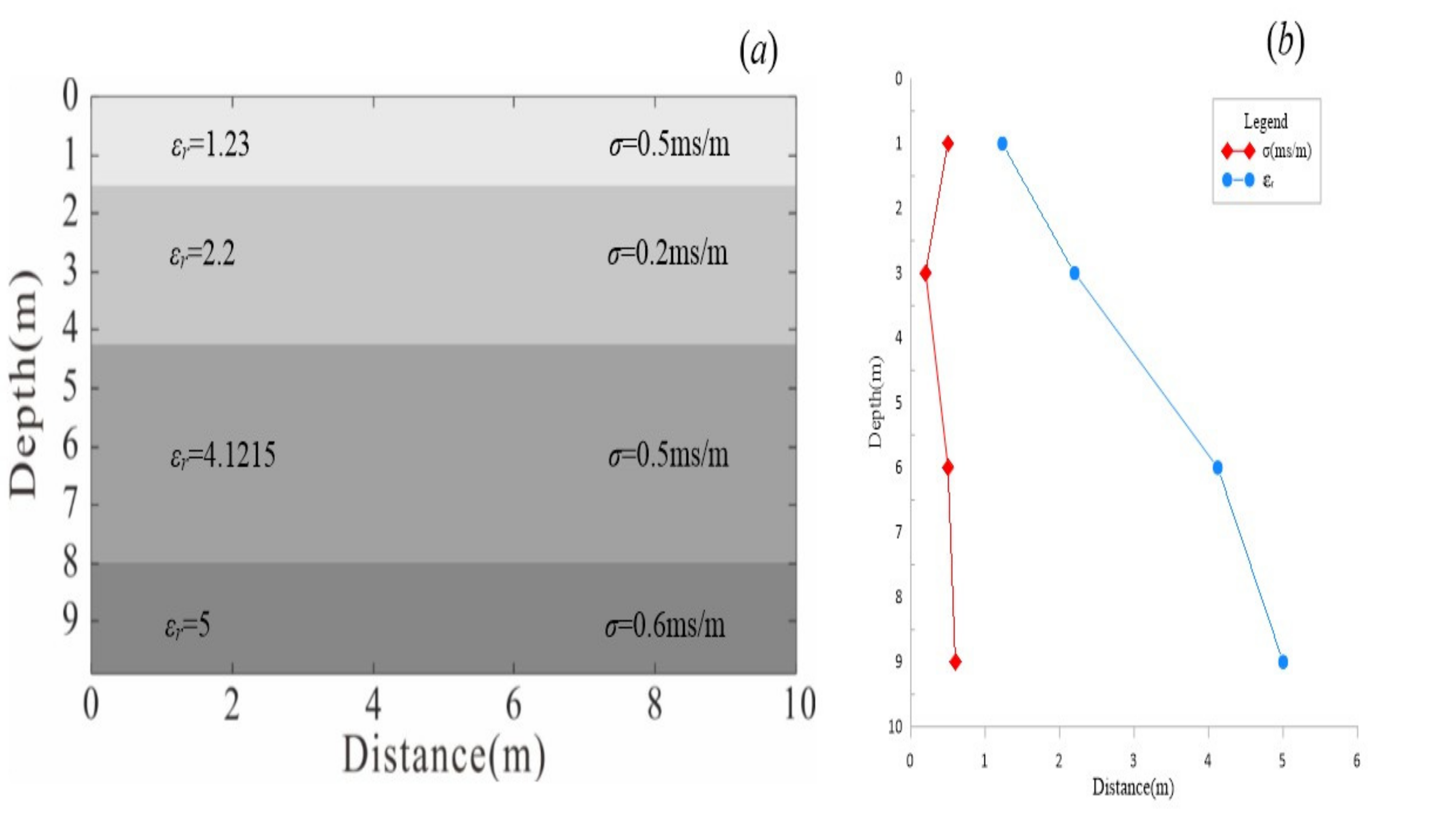
Although GPR and reflection seismic do not share common physical and methodological bases, both share similar processing and interpretation techniques. In our study, we have used all those expressions which are valid for reflection seismic considering the sensitivity, and the same mathematical expressions will be used to calculate the synthetic velocity models. The AVO velocity values are very close to the experimental values obtained using the dielectric constant technique, confirming the results of our proposed method. The experimental velocities are also similar to the common depth point (CDP) values but do not match as AVO, confirming the study’s main goal. Additionally, at certain points, there is an abrupt change in the velocity, and the reason for this is the changing lithology.

The time difference (Δt) is a function of the source-receiver offset ($x$), as typically in GPR literature this is related to arrival time at two different offset positions ($x$), zero-offset travel time ($t_0$) and velocity error (ΔV). In reality, ΔV is the difference between the rate of change of the original position of a source antenna component and the rate of change of the receiving antenna. It is referred to as the angle of incidence. The time difference (Δt) is given in Equation (1). From Equations (1)–(5), the whole mathematical process is given for the horizontal subsurface reflectors. This means, whenever the velocity model of horizontal reflectors is designed, these equations come into play. The below mathematical calculations have been explained in detail by [21].

$$\mathsf{\Delta }t={\left(\sqrt{\frac{x}{v}*\Delta v}\right)}^2+t_0-\sqrt{{\left(\frac{x}{v}\right)}^2+t_0{}^2}$$

(1)

The above equation can be approximated by a truncated (McLaurin) series. We will use polynomials in the form of truncated (McLaurin) power series to approximate functions with a definite accuracy. Since we are concerned with the shallow surface where the small variation of the incident angle is compared with the deep surface, that is why we assume Δv ~ 0.

$$\mathsf{\Delta }t=\mathsf{\Delta }v\frac{\partial \left(t\right)}{\partial \left(v\right)} |\Delta v=0$$

(2)

Evaluating this differential by assuming a zero-velocity error, we obtain

$$\mathsf{\Delta }t=-x^2\mathsf{\Delta }v/v^2\sqrt{x^2+{\left(t_{0}v\right)}^2}=-t\sin \left(\mathsf{\theta }\right)\tan \left(\mathsf{\theta }\right)\Delta v/v$$

(3)

$$v=-t_0\frac{\mathsf{\Delta }v}{x} A\prime \left(t\right)\sin \left(\mathsf{\theta }\right)\tan \left(\mathsf{\theta }\right)$$

(4)

Equation (4) is the most important equation in our case. All the terms are definable. It clearly describes the effect of angle in velocity determination. Here source-receiver offset is ($x$), zero-offset travel time is ($t_0$), and velocity error is (Δv). Additionally, A′(t) is the time derivative of the zero-offset response, where θ is the effective incidence angle which can be calculated as follows,

$$\mathsf{\theta }={\tan }^{-1}[\frac{x}{v{t}_0}]$$

(5)

WARR gather is strictly followed during the data acquisition.

The separation between the antennas is varied, keeping the center position of the antennas constant. With varying separation and assuming a layered subsurface structure, various signal paths with the same point of reflection are obtained. Supposing we will encounter dipping reflectors, we can establish all those mathematical expressions to explain the velocity of dipping reflectors and hence provide the AVO and CMP velocity models. Effects of dipping reflectors have been discussed by several researchers. Dip moves out (DMO) correction is an extension to the NMO correction when dips are present [22]. As shown by [23], the travel time to and from the reflector is given by

$$v^2{t}^2=4d^2+X^2-4dX\cos \propto$$

(6)

In Equation (6), $v$ is the velocity of subsurface, t is travel time, and $X$ is the offset while $d$ is the distance to the reflectors while $\propto$ is apparent incidence angle to the dipping reflector.

Now if we rewrite this equation in the simplest form in the terms of (D), the given results are

$$t^2={\left(2D|V\right)}^2+{\frac{X^2}{V^2}}_{NMO}$$

(7)

Hence, in this Equation (7), there is a term used ($v_{NMO})$ which is known as apparent velocity, and it is different from the velocity ($v),$ and is defined as

$$v_{NMO}=\frac{v}{\sin \alpha }$$

(8)

Equation (8) indicates that events that have bounced about in a near-surface, relatively low-velocity layer have greater normal moveout than primary reflections when both occur at the same record time. The above equation, given by Becht, Appel and Dietrich [21] is used for the dipping interface and can be further simplified as well.

2.2. Data Acquisition

The GPR antennas were positioned 1 m apart and were oriented in a broadside configuration. After examining the profile, an appropriate location for a CMP sounding, away from any point distribution in the subsurface, was determined. The CMP sounding was performed by progressively increasing the separation (the Tx–Rx offset) of the antennas in steps relative to the selected midpoint location along with the original profile. For the AVO data collection, we made slight changes, the step size of zero was approached, and the antenna was oriented 2 m apart. AVO data acquisition is the most critical partof the process and is more difficult compared to CMP data collection. We need to move the receiving antenna with great precision because if the offset variation is too large or too small, the requirement of the method is not met. The field parameters are given in

Table 1. GPR data acquisition parameters and geometric values used for AVO and CMP gather generation.

Parameters	Values
a. Step Size	0.1 m and 0.00
b. Stacking	64
c. Sample Rate	0.6 ns
d. Time Window	500 ns

. With the above data acquisition method, we suggest that the most accurate results can be obtained in the future if the step size approaches zero since the minimum step size yielded accurate results.

2.3. Data Processing

We assessed three methods for estimating velocity from CMP data. The GPR signal velocity can be determined by picking the first-break arrivals from the observed two-way travel time (TWT) for specific directions and reflected phases [21]. These picked arrivals were then analyzed using either linear moveout (LMO) analysis (for the direct and refracted phases) or NMO analysis (for the reflection phases). Trend lines were fitted to the observed arrivals using a least mean squares approach in either linear or squared space for LMO or NMO analysis, respectively. For AVO, we tended to adopt NMO analysis because AVO yields bright spots in deep investigations.

CMP gathers show a hyperbolic reflection pattern, which was used for the velocity modeling. Static correction/muting was applied to mute the unused multiple; trace interpolation was applied to resort to the signals, and time to depth conversion was also applied. We used a time window up to 200ns, whereas the AVO gathers yield the two following results: the clear reflector position and the exact velocity change values. Finally, a cutoff method or complex trace analysis/spectral analysis was applied to find out the accurate velocity. The best resolution was also determined during our processing. During processing, we came to know that first-arrival tomography is one way for building a subsurface. Reflection tomography will add deep information into the analysis. Combining both will improve the reconstruction when lateral variations are important beyond CMP approximations. With the same method using AVO data, not only the picture is clear but additional information can be extracted easily and accurately. AVO could provide unique information if taken care of the source effect and the topography influence. However, it requires clear phase identification for recovering a better model.

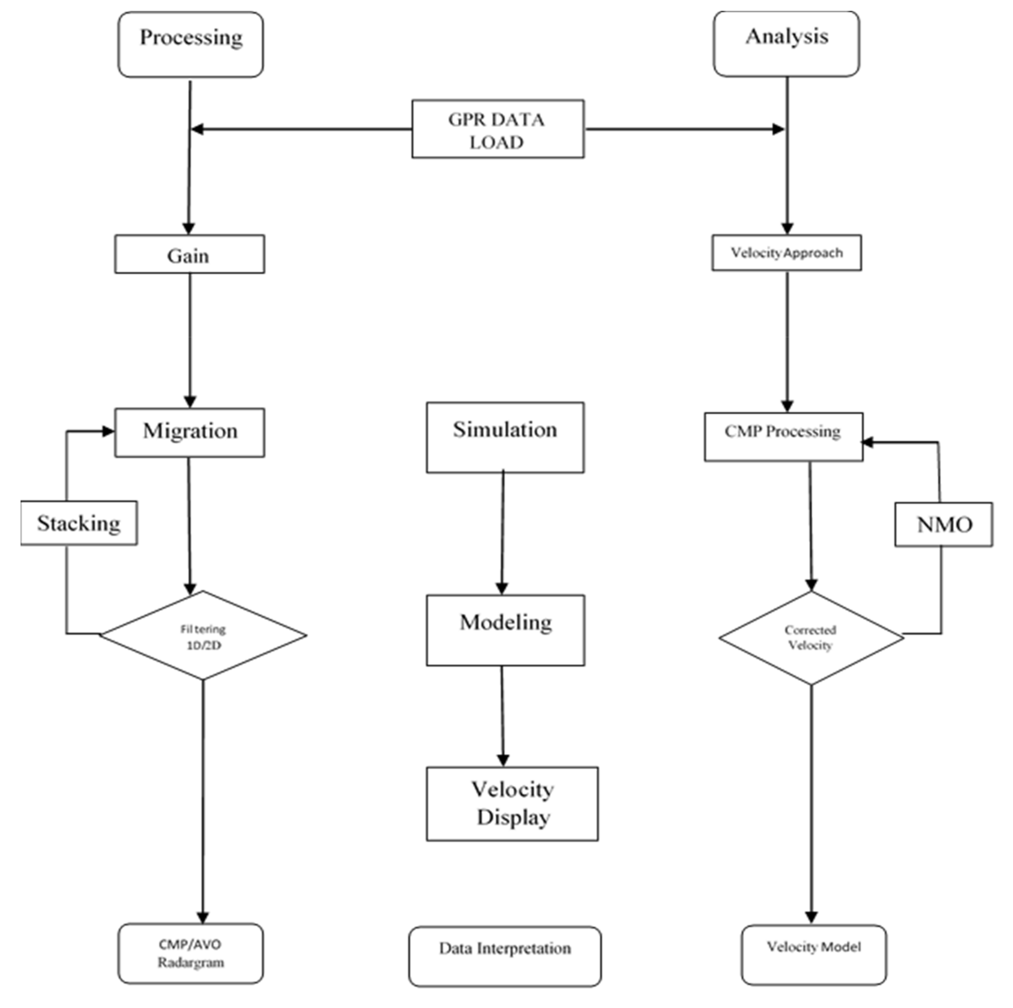
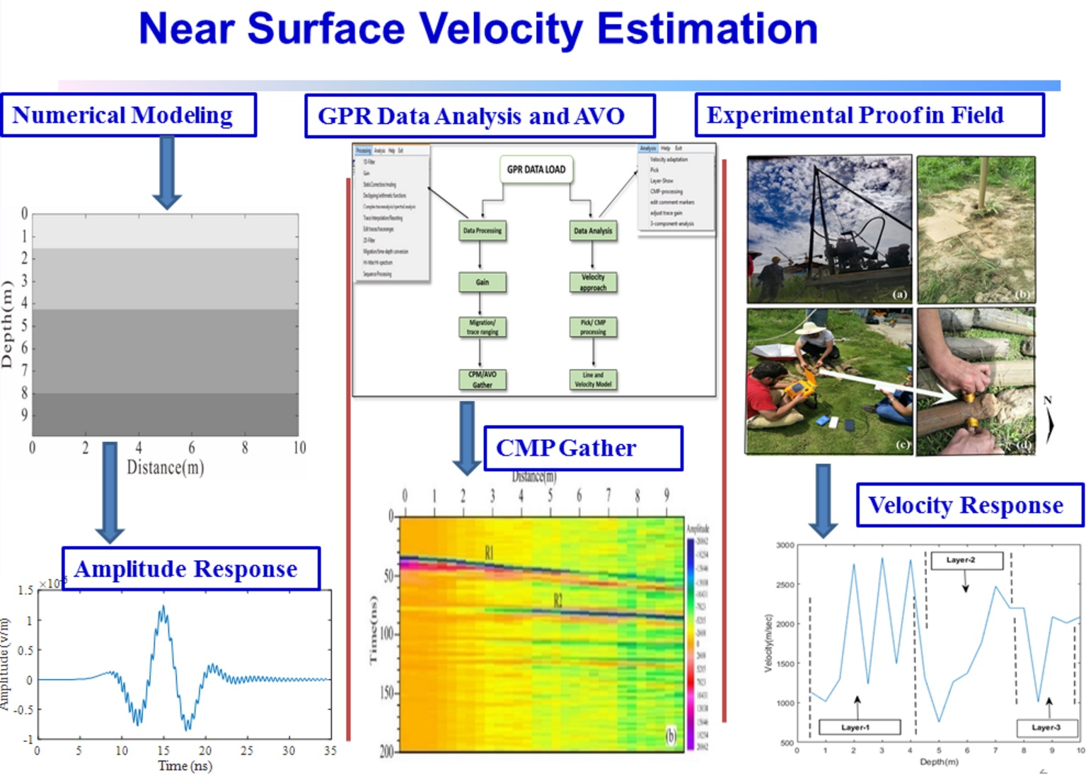
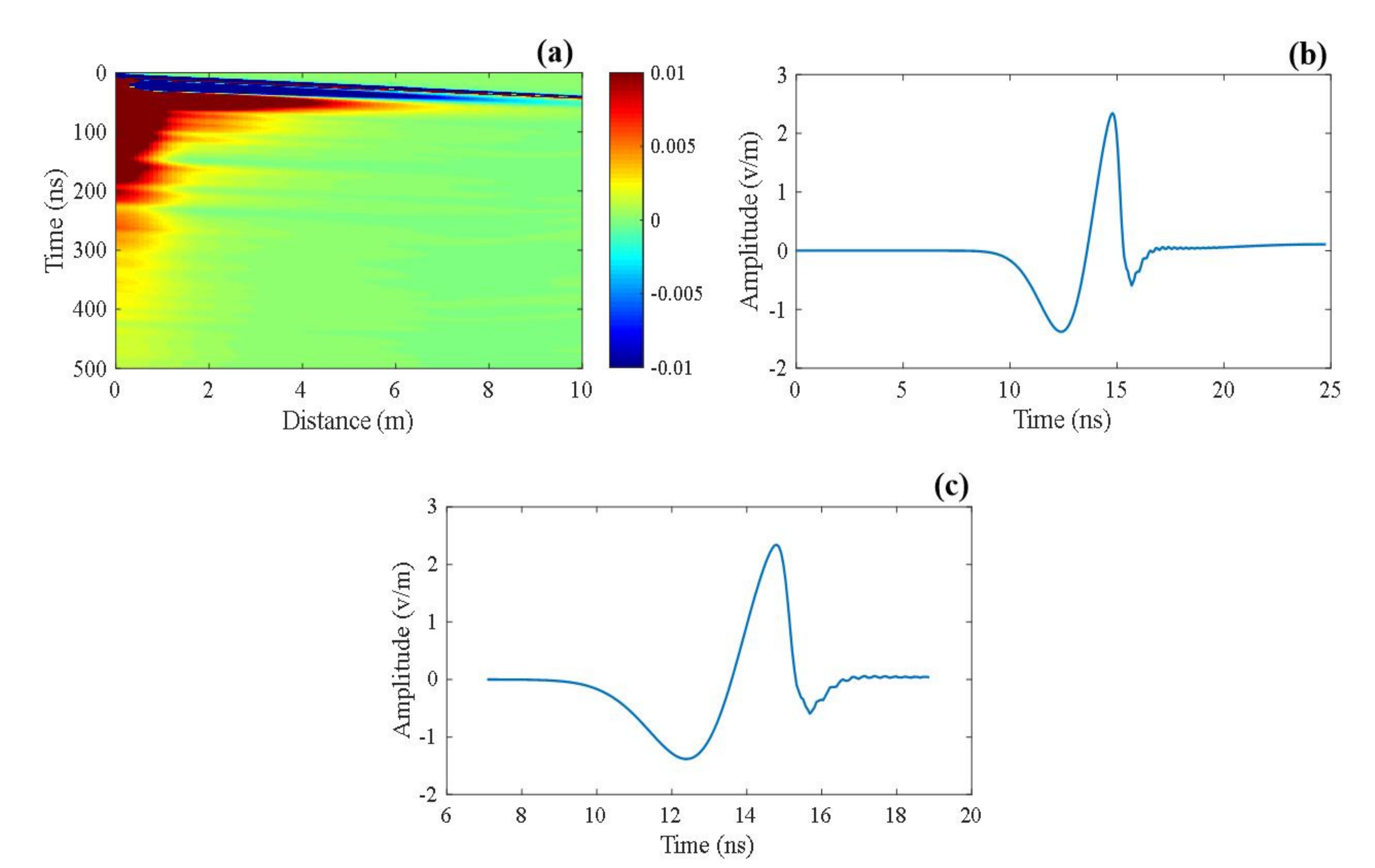
From the following analysis, we determined the velocity cut-off point. The precision of the radar wave’s velocity and the TWT at zero offsets were then estimated from the picked TWT data by using Student’s t-test at the 95% confidence limit [24]. Figure 1 shows the data processing flow chart. The whole data processing and analysis are done by using REFLEX_W, MATLAB, and EKKO_VIEW Deluxe software.

3. Results and Discussion

3.1. Numerical Simulation Analysis

Hilbert transformation of the signal acquired in the given number of channels is the two-way travel time, which is given by

$$ti=\frac{\sqrt{x{i}^2+4d^2}}{v}$$

(9)

where x denotes the distance between the transmitting and receiving antennas in the i-th channel, d denotes the depth to the horizontal reflection interface, and v denotes the velocity of electromagnetic waves propagating in the stratified layer above the reflection interface.

We can select the stacking velocity from the velocity spectrum, which can be approximated as the root mean square velocity. The velocity spectrum was smoothed before picking the stacking velocity to make it easier to pick. The Dix equation [25] can then be used to calculate the interval velocity in each layer:

$$Vint,i= \sqrt{\frac{V^{2}st,i+1ti+1-V^{2}st,iti}{ti+1-ti}}$$

(10)

where Vint denotes the interval velocity in the i-th layer, and Vst. j and t denote the stacking velocity and two-way vertical travel time of the i-th selected reflection event, respectively. The depth of the i-th layer can then be calculated as follows:

$$di=Vi\left(ti+1-ti\right)$$

(11)

As a result, we can estimate the vertical profile of the interval velocity of layered media, which can be converted into the vertical distribution of dielectric permittivity, which can be related to soil water content, for example. Velocity adaptation leads to the pick velocity of the reflectors. After that, we do CMP-modeling as shown in Figure 2a, which gives a complete velocity model. This model is generated using GPR Max2D based on the above-explained mathematics and the following parameters: relative permittivity and electrical conductivity. Our simulated model is divided into four layers that represent four different subsurface materials: dry sand, clay, granite, and clay again. In the following section of this paper, we assumed the values given in the model on good insight of the test site, which will be used for drilling and synthetic study. Because we know that representational graphics can quickly illustrate general behavior and highlight phenomena, anomalies, and relationships between data points that might otherwise be overlooked and may contribute to predictions and better, data-driven decisions, Figure 2b is a graphical representation of our mathematical model that helps to clarify the subsurface picture.

We use velocity spectrum analysis to ID inversion the dielectric properties of layered media based on the CMP data. We use an algorithm of unnormalized cross-correlation sum [26] to calculate a velocity spectrum, which is given by the following equation [27].

$$CC\left(\tau ,v\right)={{\displaystyle \sum }}_{i=1}^{N-1}{{\displaystyle \sum }}_{j=i+1}^N fi\left(ti\right)fj\left(tj\right)+gi\left(ti\right)gj\left(tj\right)$$

(12)

where CC is the unnormalized cross-correlation sum, Ni is the total number of channels (offsets) in a CMP gather, I and j are the offset indices, t is the two-way zero-offset travel time, v is the trial velocity used to calculate the velocity spectrum, and f(t) and g(t) are the real and imaginary parts of the analytic signal, respectively. As is shown in Figure 3a, there is clear velocity contrast while simulating the velocity according to the physical properties of near-surface materials. The corresponding velocity amplitude spectrum with maximum velocity amplitude at 14ns is shown in Figure 3b; hyperbolic curves over the CMP profile are the travel time-distance curves of the direct coupling and reflection signal calculated from the velocity estimates, respectively, as shown in Figure 3c: 3 (a) The simulated velocity model of subsurface materials; 3 (b) the corresponding velocity amplitude spectrum with maximum velocity amplitude at 14ns is also shown in the figure; 3 (c) the corresponding velocity amplitude curve with shift caused by the introduction of the next interface, with maximum velocity spectrum at 15 ns. The fitted hyperbolic curve calculated from the selected reflection event is the curve over the CMP profile. The travel time–distance curves of the direct coupling and reflection signals calculated from velocity estimates are represented by hyperbolic curves over the CMP profile.

3.2. GPR Data Analysis with Amplitude Variation with Offset (AVO)

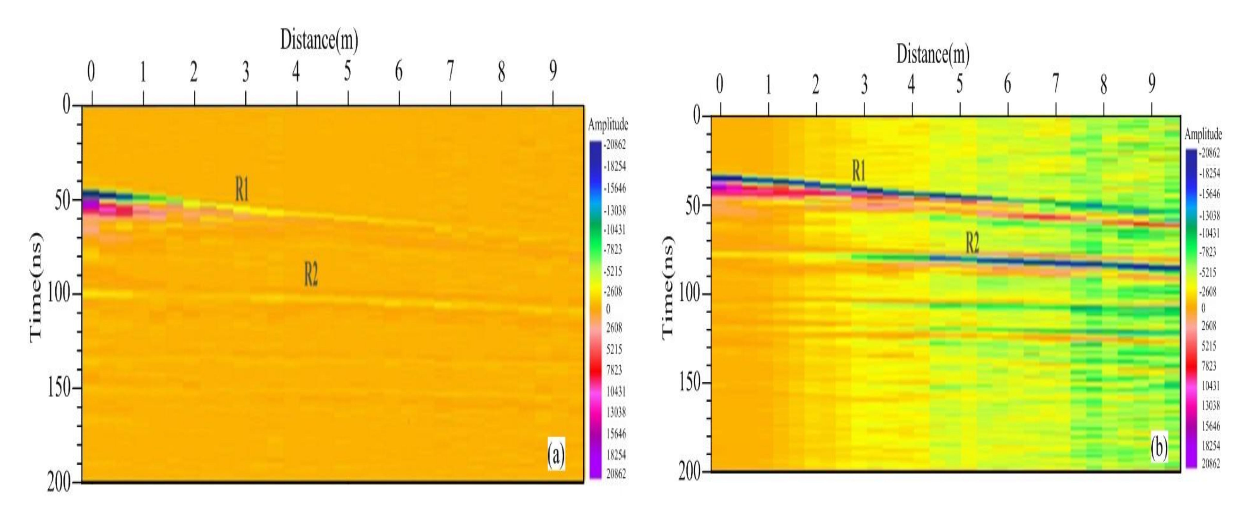
Across the traverse, the raw GPR profile shows continuous reflections from both flat-lying and dipping interfaces, as well as several diffraction patterns indicative of points embedded in the subsurface. Surprisingly, the hyperbolic velocity analysis of three possible diffraction patterns shows variable tail spreads, indicating lateral and vertical changes in GPR signal velocity. There are two main conclusions from our initial judgment: first, reflectors 1 (R1) and reflector 2 (R2) are located in the shallow subsurface, and second, this is observed on the CMP gather as shown in Figure 4a,b, which represent both pre-and post- stack images that are obtained from the CMP gathers.

However, the results of AVO are clear; therefore, in comparing the results of the CMP method and the AVO method, we conclude that AVO is superior for near-surface velocity estimation. Although rapid vertical velocity changes may be present due to typical sedimentary, hydrological, and archeological layering, strong reflections are also created by the interfaces, which can be observed in the GPR AVO profile in Figure 4a.

A wide range of GPR signal velocities over a short profile distance raises concern about the accuracy of estimation of velocity but can also be representative of the type of heterogeneity found in many archaeological settings [28]. However, we observe that several of the diffraction patterns share traces with adjacent diffraction patterns, for example, reflector (R1) and reflector (R2) in Figure 4b. Here, again function is applied during data processing. When the gain was applied to the raw data, the reflectors were clearer. In our case, when we applied gain then applied the stack correction, we observed while in the CMP gather, only one reflector is visible, and we cannot distinguish between the other reflectors.

However, when the same process is applied with AVO data processing, we could distinguish between the upper and lower reflectors. According to these results, there is a marked lithology contrast between the upper and lower reflectors. The lower reflector had a small dip for its original position, and therefore, migration was also applied. In the analysis portion of our processing, we used the velocity adoption method for both types of gathers. Finally, we obtained the velocity model from the data processing.

From Figure 4a, we can predict that layering is present in the subsurface, while for Figure 4b reflectors are observed, but it is difficult to distinguish them. In the case of AVO, the reflectors are both quite clear and distinguishable as follows.

From Figure 4a, more than one reflector is observed, but the individual reflectors cannot be distinguished, while in Figure 4b, reflectors are not only distinguishable but we can also see their clear position and velocity; therefore, it can be observed that AVO processing yields a better image.

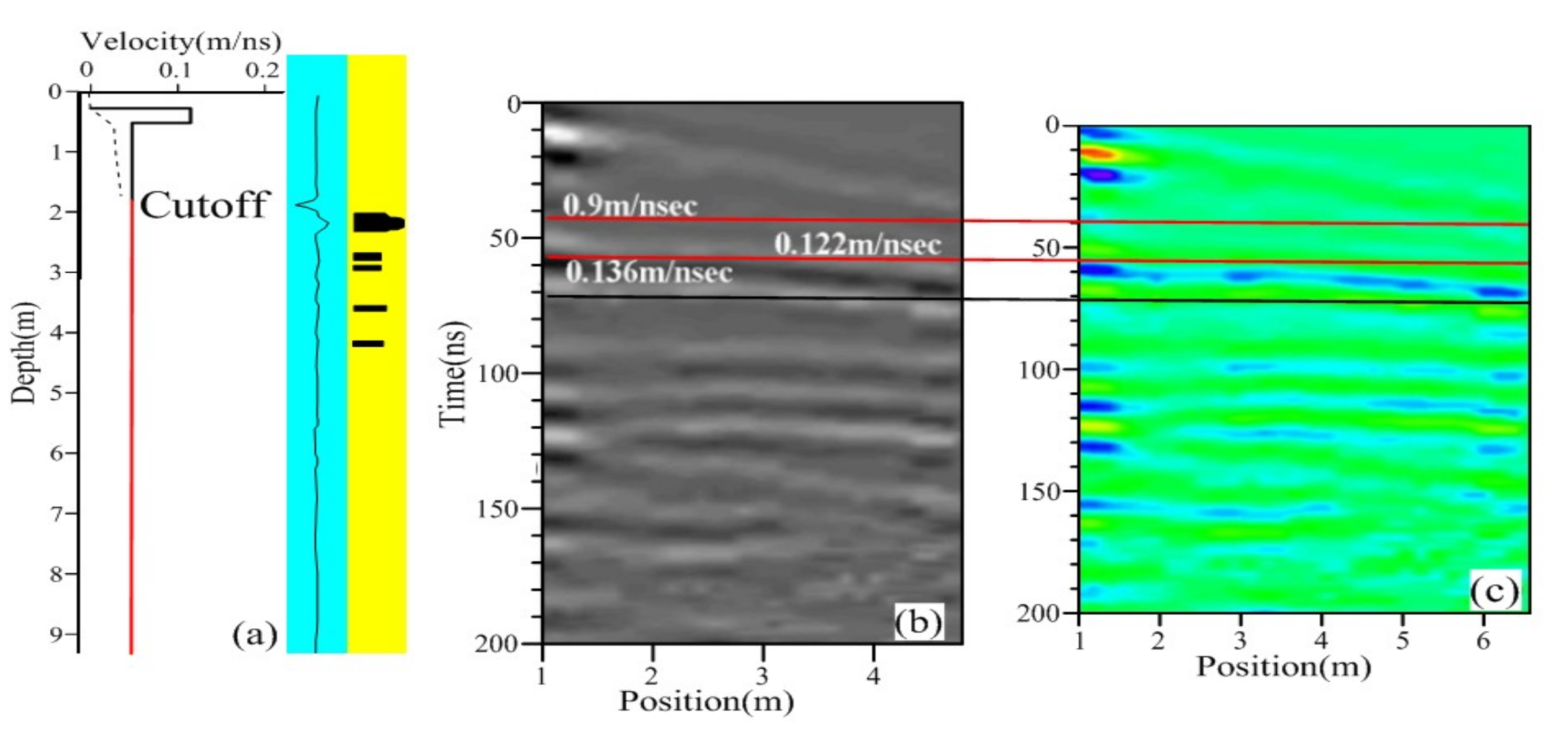
The normal electromagnetic (EM) velocity ranges from 0.07 m/ns to 0.15 m/ns, which is consistent with the literature. The GPR signal velocity from the hyperbolic velocity analysis ranges between 0.02 m/ns and 0.1 m/ns over 10 m of the profile, which is the case for the CMP gathers. These results may indicate that there is a change in velocity with depth, whereas the shallow point scatterer indicated a velocity of 0.22 m/ns, while the deeper point scatterer showed a velocity of 0.07 m/ns. While processing our data, we observed differences in the velocities between CMP and AVO processing.

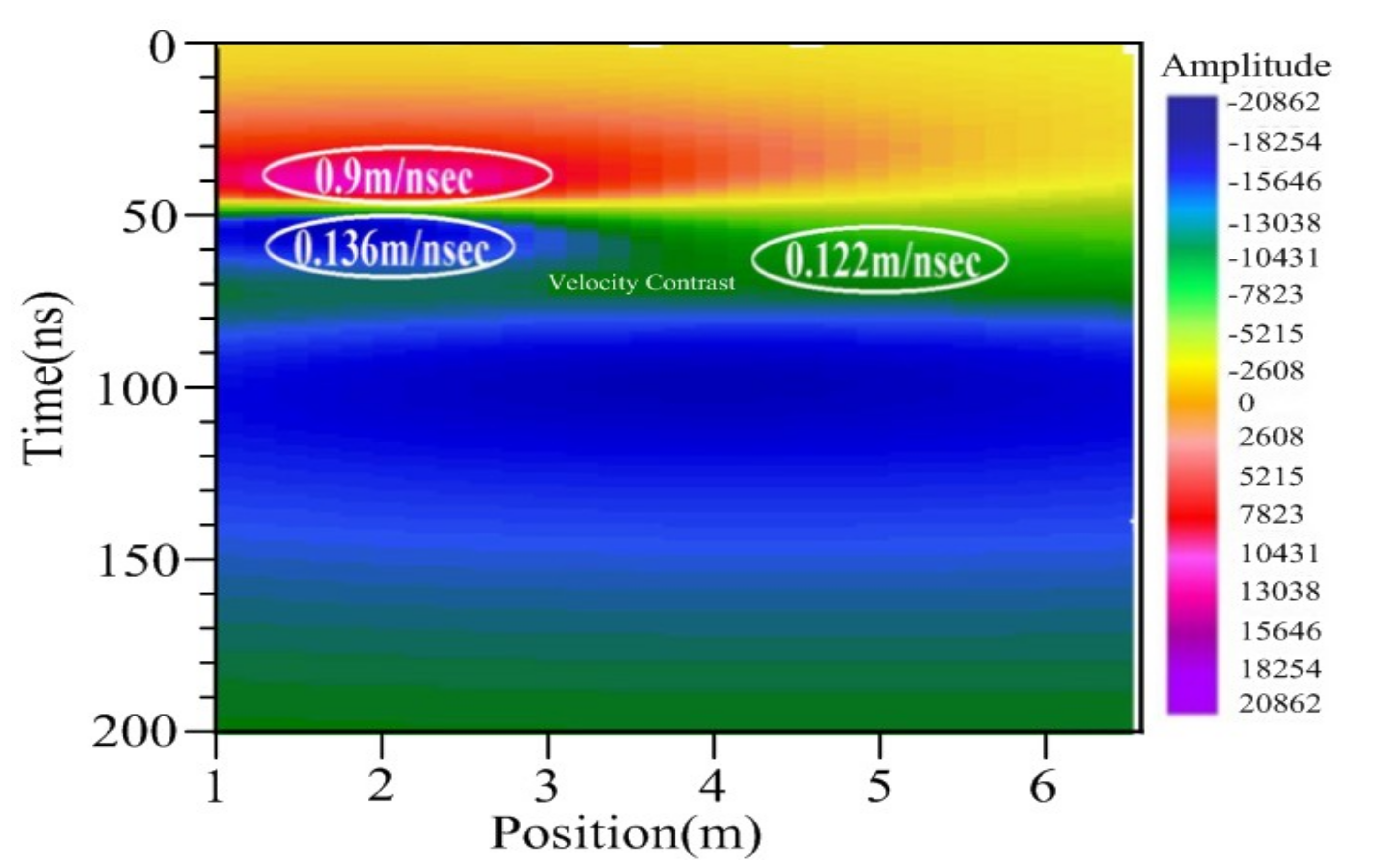
Figure 5 presents the 2D velocity model with three different colors in the model that show the appropriate velocity variation in the target area. The color contrast in the figure indicates two major phenomena: first, the increasing velocity trend, and second, the different velocity values with changing reflectors. In the velocity model above, three color-coded velocities have been marked due to contrast, and they are 0.02 m/ns, 0.04 m/ns, and 0.06 m/ns. To verify these results, the velocity values are compared with the field data.

We computed two velocity models, one from the common mid-point data and the other from amplitude variation with offset data processing. The primary difference between the models was that the common offset model was a poor representation of the subsurface, while the AVO data model showed clear features. There should be a velocity pattern in the subsurface, which can easily be seen in the amplitude variation with offset data, but it is not clear in the CO velocity model. The AVO velocity model has one general trend, which is known as the correlation. The clear depth of the reflectors is obtained by correlating the velocity line with the model and the pre- stacks data, as shown in Figure 6 (a, b and c). The velocity model shows that the first velocity increases, but when the waves hit the reflector, the trend becomes constant; this pattern is repeated for the subsequent waves.

3.3. Experimental Velocity Analysis

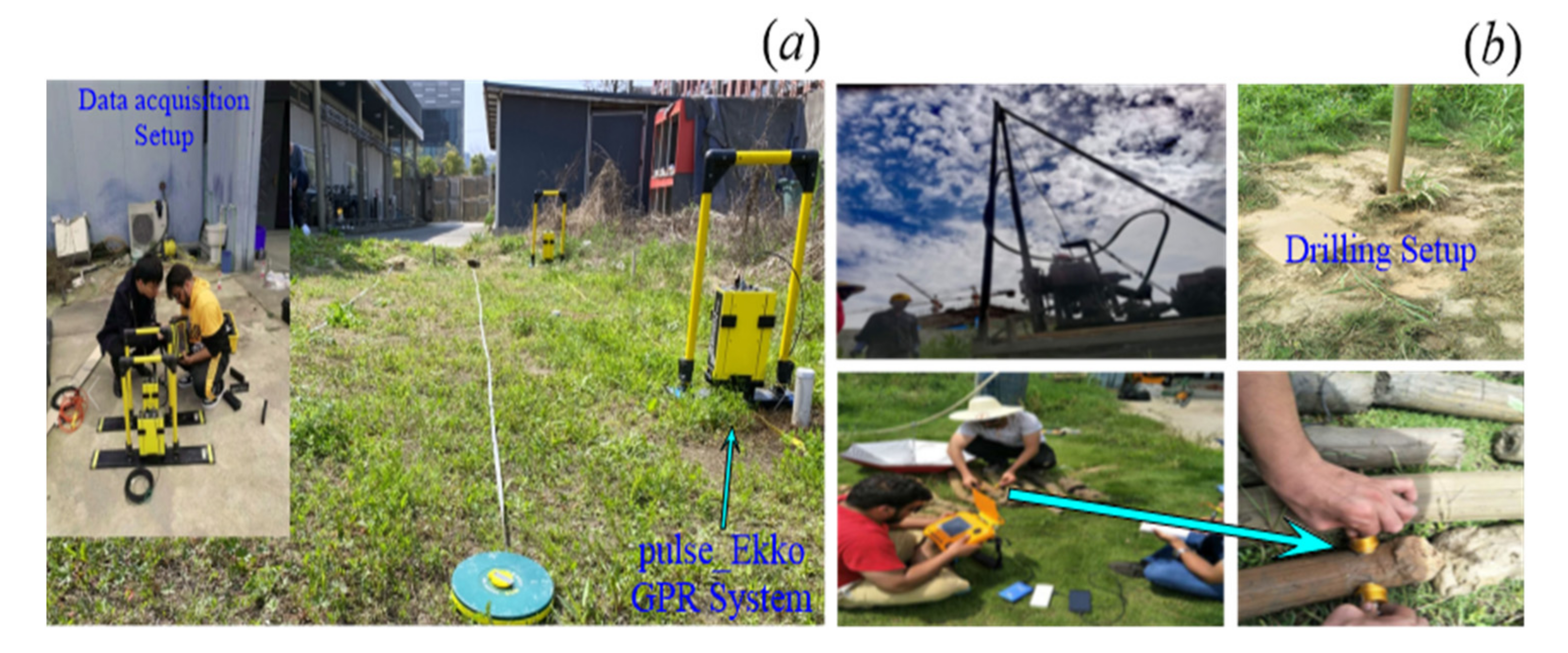
We used a pulse EKKO GPR system (Sensors and Software Inc.) with bi-static 50–200 MHz unshielded GPR antennas, and a single operator with WARR complete data acquisition setup can be seen in Figure 7a.

To verify the previous results, we conducted a field experiment. In the experimental site, a drilling well 10-meter deep and approximately 2.9 cm diameter was drilled to collect subsurface samples for the validation analysis ground truthing Figure 7b.

Velocity is related to permittivity and resistivity, but the values of velocity are most reliable when they are acquired using the permittivity or a dielectric constant. An established procedure can be used to estimate the electromagnetic (EM) velocity using ground-penetrating radar (GPR) data; we can also estimate the velocity both theoretically and practically but using a different method. The technique is based on the inversion of reflection amplitudes to compute the series of reflection coefficients used to estimate the velocity in each interpreted layer.

The proposed method recursively calculates the incident angles at all interfaces, taking into account the offset between antennas; the input method requires the picked amplitudes values, a reference amplitude for each analyzed GPR trace and a velocity value for the shallowest layer [29]. The method produces two results, the velocity trend and the velocity of every layer. We used the method for the velocity calculation and to verify the results as follows.

As Figure 5 shows, the 2D velocity estimation does not show a clear velocity contrast depth. Up to 5 m depth, there is small contrast in the velocity with changing lithology, but the contrast is abrupt due to the presence of anomalous material in deeper. In our case, the contrast is due to the changing lithology at every meter, as observed with several samples collected from the borehole.

3.4. Velocity Estimation Using Dielectric Constant

The velocity that is calculated using the supersonic instrument may not be reliable due to error, but to avoid these errors, we decided to generate the velocity curve using the dielectric constants of the samples collected during our drilling. The instrument used to measure the permittivity of the sample is the parameter v.7 with the frequency of 40–50 MHz; moreover, the Display is LED, the Range of a parameter is 1–99.9 mS/cm; resolution is about 0.1 mS, and Power is 12 V. The Digital Percometer is a reliable, accurate, lightweight, and easy-to-use instrument for measuring the dielectric value, electrical conductivity, and temperature of materials indoors. A similar method has been applied to determine the dielectric constant of the material, i.e., 2 values per sample with a spacing of approximately 0.5 m. The mathematical expression used in our calculations is given as

$$V=c/{\left(\epsilon r\right)}^{0.5}$$

(13)

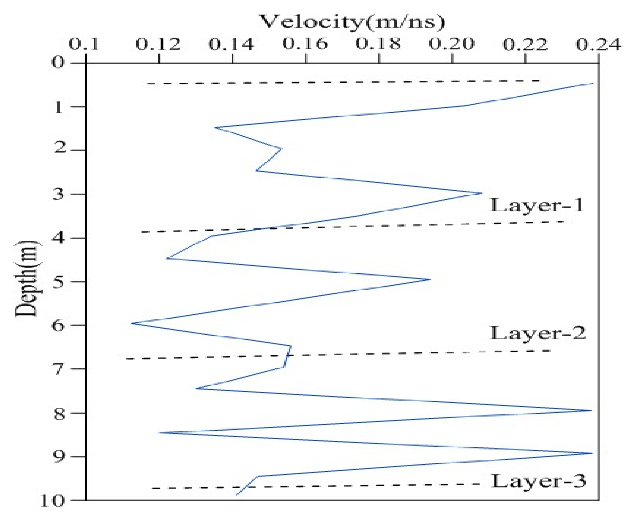
where ($c$) is the speed of light, and ($\epsilon r)$ is the dielectric constant of the material. The above equation, which is considered as a modified Maxwell equation, is well defined in the literature, e.g., [30]. The result of the calculation is shown in Figure 8. The figure shows that the velocity trend is similar to that of a 2D model and that of the supersonic instrument; however, the result closer to that of the model than to the electromagnetic (EM) velocity measurements.

One velocity trend is observed in the experimental calculation. First, the velocity values are changing with depth. Second, we observe the constant fluctuation with increasing depth and velocity that varies from 1 to 8 m depth, which is almost equal to the synthetic values we obtained earlier in our studies. With the dielectric constant, there is an abrupt change of 5 m depth, and this change corresponds to the values predicted in our synthetic study. It has been shown in the past that using this technique, the range of velocity is normally 0.07 to 0.25 m/ns. We see that our results, which range from 0.11 to 0.23 m/ns, are similar to the calculated values. This verifies that our results are accurate, and therefore, we can endorse the AVO method over any other geophysical technique to determine near-surface velocities. Based on the above calculations and discussions, we present the velocity distribution of the subsurface media at the test site in

Table 2. Velocity comparison of CMP, AVO, and experimental data.

Depth (m)	AVO Velocities (m/nsec)	CDP Velocities (m/nsec)	Lithology For the Dielectric Constant	Experimental Velocities via Dielectric Constant (m/nsec)
1.0	0.1152	3.9	Dry Sand Stone	0.23717
1.5	0.300	4.121	Dry Sand Stone	0.20226
2.0	0.965	4.1	Wet Sand Stone	0.13553
2.5	0.123	4.52	Wet Sand Stone	0.15390
3.0	0.500	5.0	Clay	0.14639
3.5	0.366	0.56	Wet Clay	0.20702
4.0	0.136	0.122	Wet Clay	0.17617
4.5	0.120	0.125	Wet Clay	0.13416
5.0	0.139	0.622	Wet Clay	0.12247
5.5	0.1639	0.750	Clay	0.19365
6.0	0.122	3.1	Granite	0.15191
6.5	0.600	3.1	Wet Granite	0.11310
7.0	0.160	3.1	Wet Granite	0.15596
7.5	0.4213	0.45	Clay	0.15390
8.0	0.1222	0.52	Wet Clay	0.1300
8.5	0.2121	0.52	Wet Clay	0.23717

. The transit time for 2.6 m of travel is 40 to 60 ns. This may indicate that the geological structure is a clay material with some water saturation. Otherwise, consider a dry sand ε = 5 with conductivity σ = 5 mS/m. The expected velocity is 0.15 m/ns, and the attenuation is 3.8 dB/m which corresponds to a distance of 26–27 m for 100 dB of attenuation and a travel time of 100ns or longer due to the presence of reflectors from 100 to 150 ns. This example might correspond to dry sedimentary rocks, such as divisions in clay, compact clay, and sandstone. From the above observations, we divided our site into three layers containing freshwater in their pore spaces. The results of the experiments become less valid as conditions vary from the initial assumptions (i.e., σ > 10 mS/m and µ ≠ 1) due to the dispersive effect of conductivity and the added influence of relative magnetic permeability on wave propagation.

These large variations in velocity and attenuation are the cause of success (target detection) or failure (insufficient penetration) for surveys in similar geologic settings. Since comprehensive catalogs of the properties of specific earth materials are not readily available, most GPR work is based on trial and error and empirical findings. The assumptions of low-conductivity and nonmagnetic material are valid for most nonclayey, sedimentary materials.

4. Conclusions

Precision velocity model estimation is critical for high-quality GPR surveys. Many methods have been used in the past for velocity estimation, but many do not yield good results in certain field conditions. Here, we have suggested that by using the AVO velocity estimation method, we can also observe the maximum resolution point by determining the cut-off from the amplitude spectrum; this method has been successful for both single and multi-traces. We have observed that our velocity models are not only important for applications in archeological sites but can also be used for water-saturated areas, especially where there is any kind of lithology under the water table. Finally, our field experiment provides the general trend of the velocity in the near-surface, and the field experiment shows that the AVO velocity estimation is superior compared to that of the CDP.