Article

Inverse Synthetic Aperture Radar Sparse Imaging Exploiting the Group Dictionary Learning

1
Key Laboratory of Radar Imaging and Microwave Photonics, Ministry of Education, Nanjing University of Aeronautics and Astronautics, Nanjing 210016, China
2
Center for Sensor Systems, University of Siegen, 57176 Siegen, Germany
*
Author to whom correspondence should be addressed.
Remote Sens. 2021, 13(14), 2812; https://doi.org/10.3390/rs13142812
Submission received: 20 May 2021 / Revised: 30 June 2021 / Accepted: 15 July 2021 / Published: 17 July 2021

Abstract

:
Sparse imaging relies on sparse representations of the target scenes to be imaged. Predefined dictionaries have long been used to transform radar target scenes into sparse domains, but the performance is limited by the artificially designed or existing transforms, e.g., Fourier transform and wavelet transform, which are not optimal for the target scenes to be sparsified. The dictionary learning (DL) technique has been exploited to obtain sparse transforms optimized jointly with the radar imaging problem. Nevertheless, the DL technique is usually implemented in a manner of patch processing, which ignores the relationship between patches, leading to the omission of some feature information during the learning of the sparse transforms. To capture the feature information of the target scenes more accurately, we adopt image patch group (IPG) instead of patch in DL. The IPG is constructed by the patches with similar structures. DL is performed with respect to each IPG, which is termed as group dictionary learning (GDL). The group oriented sparse representation (GOSR) and target image reconstruction are then jointly optimized by solving a l 1 norm minimization problem exploiting GOSR, during which a generalized Gaussian distribution hypothesis of radar image reconstruction error is introduced to make the imaging problem tractable. The imaging results using the real ISAR data show that the GDL-based imaging method outperforms the original DL-based imaging method in both imaging quality and computational speed.

Graphical Abstract

1. Introduction

Inverse synthetic aperture radar (ISAR) can obtain high resolution images of moving targets in all weather, day and night. It is an important tool for target surveillance and recognition in non-cooperative scenarios [1]. Traditionally, ISAR imaging uses the range-Doppler (RD) type of methods. Under the assumption of a small rotational angle, the cross-range imaging is achieved by fast Fourier transform (FFT). If the targets undergo complex motion, the imaging time needs to be selected or the high-order motion needs to be compensated. The imaging results of this type of method usually suffer from sidelobe interferences.
The sparsity-driven radar imaging methods have verified that incorporating the sparsity as prior information in the radar image formation process is able to cope with the shortcomings of the RD type of methods. These sparsity-driven imaging methods [2,3,4,5,6,7,8,9] assume that the target scene admits sparsity in a particular domain. In particular, regularized-based image formation models focus on enhancing point-based and region-based [2,3,4,5,6] image features by imposing sparsity on features of the target scene, whereas sparse transformation-based image formation models [7,8,9] represent the reflectivity fields sparsely with dictionaries by imposing sparsity on the representation coefficients through the dictionaries. Both models have been shown to offer better image reconstruction quality as compared to traditional RD imaging methods. However, the aforementioned ways for sparsifying the target scene only depict pre-defined image features and are not adaptive to the unknown target scenes; the performance is, therefore, limited.
In contrast to dictionaries constructed with fixed image transformations used in sparse transformation based image formation models, the dictionaries obtained by the dictionary learning (DL) technology [10,11,12,13] are generated with the prior information of the unknown target image. Thus, the learned dictionaries are adaptive to the target images to be reconstructed and can find the optimal sparse representation coefficients [14,15]. Nevertheless, the strategy of processing each target scene patch independently during the DL and sparse coding stages neglects the important feature information between the patches, such as the self-similarity information which has been proved to be very efficient for preserving image details [16,17,18,19,20] during the image formation process. Both DL and sparse coding stages are calculated with relatively expensive nonlinear estimations, e.g., orthogonal matching pursuit (OMP). These two deficiencies actually limit the improvement of the reconstruction quality and efficiency of DL-based ISAR sparse imaging, respectively.
In order to exploit self-similarity information between patches to recover more details of the target image, we adopt the image patch group (IPG) instead of the independent patch as the unit in DL and sparse coding stages. The IPG is constructed by the patches with a similar structure. A singular value decomposition (SVD) based DL method is performed with respect to each IPG, which is termed as group dictionary learning (GDL). The group-oriented sparse representation (GOSR) and target image reconstruction are then jointly optimized by solving a l 1 norm minimization problem exploiting GOSR, during which a generalized Gaussian distribution hypothesis [21] of radar image reconstruction error is employed to make the imaging problem tractable. The initial idea of our work for ISAR imaging using GDL was presented in the conference paper [22].
Compared with the existing ISAR sparse imaging methods, the innovations of the proposed imaging method are as follows: (1) The IPGs, instead of independent patches, are used as the units in DL and sparse coding stages. The GOSRs characterize the local sparsity of target image and self-similarity information between patches, simultaneously. (2) A GDL method with low complexity is designed. The GDL is performed with respect to each IPG rather than the target image using the simple SVD. (3) An iterative algorithm combined with soft thresholding function is developed to solve the GOSRs-based l 1 norm minimization problem for target sparse imaging.
The real ISAR data are used to demonstrate the performance of the proposed GDL-based sparse imaging method. The comparisons with the greedy Kalman filtering (GKF) based sparse imaging method [9] and on-line DL and off-line DL based sparse imaging methods [15] are conducted.
The rest of this paper is organized as follows: Section 2 briefly presents the ISAR measurements model and sparse imaging model. Section 3 presents the DL-based ISAR sparse imaging methods. Section 4 elaborates the GDL-based ISAR sparse imaging method in great detail. Section 5 shows the real ISAR data imaging results and the performance analyses of our imaging method. Section 6 draws the conclusions.

2. Imaging Model

2.1. Model of ISAR Measurements

We consider an ISAR imaging geometry, including a moving radar platform and a target with both transnational motion and rotational motion, in an image projection plan (IPP). The radar first transmits a linear frequency modulated (LFM) pulsed waveform p ( t ) = r e c t ( t / T p ) e j π k a t 2 e j ω 0 t . Here, t represents the fast time, T p represents the pulse width, k a is the frequency modulation rate, ω 0 is the carrier frequency of the transmitted waveform and r e c t ( · ) is the rectangular function. The received signal from the target scene is then mixed with a reference chirp. After performing the operations of demodulation, range compression and motion compensation of higher order [23] on the de-chirped signal, the ISAR image formation can be formulated as a 2D inverse Fourier transform (FT) [9] as follows:
T ^ ( f s , τ ) r m c ( s , f t ) e j 2 π f s s e j 2 π f t τ d s d f t [ A ( f s ) T ( f s , τ ) ] ( c 2 4 f 0 Ω ) e j ω 0 τ
where f t [ B / 2 , B / 2 ] is the range frequency with B denoting the bandwidth of the transmitted waveform, f s = 2 f 0 c Ω x and τ = 2 y c , Ω denotes the effective rotational vector of the target [24], x O y denotes the local coordinate system centered at O on the target, the A ( f s ) is the spectrum of the amplitude modulation due to the azimuth antenna beam pattern, and T ( f s , τ ) is the reflectivity distribution of the ISAR target scene to be reconstructed. The r m c ( s , f t ) is the ISAR measurement after motion compensation and range compression.

2.2. Sparse Imaging Model

Let σ be the vector of the reflectivity function T ( f s , τ ) and G be the vector of ISAR measurements r m c for discrete samples of fast-time and slow-time domain. The relationship between the ISAR measurements and the reflectivity function to be reconstructed can be modeled in terms of a linear system of equations in a matrix form [9] as follows:
G = H σ + n
where H is the observation matrix of ISAR imaging. Specifically, the H is a Fourier matrix formed by H = F C F R , where F C denotes the 1D Fourier transform matrix applied to the column dimension of T ( f s , τ ) , and F R denotes the 1D Fourier transform matrix applied to the row dimension of F R . n is the noise vector embedded in the ISAR measurements. We assume that the number of samples in the range and cross-range dimensions are N r and N a , respectively. G and σ are both vectors with the dimension of N r N a , and H is a N r N a × N r N a square matrix.
The σ is naturally sparse, considering that the background of an ISAR image usually has relatively low reflectivity and the target to be imaged is a composition of a number of relatively strong scatterers. The target image can be reconstructed with measurements smaller than N r N a in the theoretic framework of CS based on the following under-determined linear systems of equations:
G s = Ψ σ + n s
where G s C m is a randomly under-sampled measurement vector, Ψ C m × n with m < n , n = N r N a is the measurement matrix, which is a partial Fourier matrix obtained by Ψ = Θ H , where Θ denotes the sensing matrix, n s is the noise vector corresponding to the under-sampled measurements G s .
The imaging problem in Equation (3) can be formulated as a space sparse constrained l 1 norm minimization model as follows:
min σ σ 1 s . t . G s Ψ σ 2 2 < ϵ
The sparse representations in the transform domains depict the certain features (point-based or region-based image features) of the interested target [7,9], thereby enhancing the imaging quality of the target scene σ . Let D C n × n be a dictionary, which sparsely represents the σ as follows:
σ = D w
where the vector w C n is sparse representation of σ in the domain expanded by D . Thus, the image reconstruction in Equation (4) is performed by obtaining the sparse representation firstly as follows:
min w w 1 s . t . G s Ψ D w 2 2 < ϵ
and then form the target image by the following:
σ ^ = D w ^
However, these dictionaries were artificially designed using the fixed image transformations and cannot be adaptive to the unknown target scene to find optimal sparse representations.

3. DL-Based Sparse Imaging

The main idea of DL-based ISAR sparse imaging is to utilize an adaptive dictionary to sparsely represent the unknown target scenes [15]. The adaptive dictionary can be learned off-line from the previously available ISAR data or on-line from the current data to be processed; the atoms in the adaptive dictionary are generated with prior information of the unknown target scene rather than the fixed image transformations.

3.1. Off-Line DL Based Sparse Imaging

A block processing strategy is adopted for reducing the size of training images to improve the efficiency of DL. Extracting the patches from a training image can be simply expressed as follows:
σ t k = F k ( σ t )
where σ t C n denotes vectorized training image, σ t k C n p denotes the k t h vectorized patch extracted from σ t , F ( · ) denotes the operator of patch extraction and k = 1 , 2 , , N is the index of the patch.
Given a set of patches { σ t k } k = 1 N , the patch-based DL can be modeled as a l 1 norm minimization problem [15] as follows:
min D p , { w t k } k = 1 N σ t k D p w t k 2 2 s . t . k w t k 1 T p
where D p C n p × n p is the patch based dictionary to be learned, w t k is the sparse representation of σ t k over the D p , and T p is the required sparsity level for each patch.
The K-SVD algorithm is used to optimize D p and w t k alternatively, leading to the optimal D ^ p . Then, the D ^ p , containing the prior information of the unknown target image, is applied to the following joint optimization problem for reconstructing the target image:
min σ , { w k } k = 1 N σ k D ^ p w k 2 2 + λ G s Ψ σ 2 2 s . t . k w k 1 T p
where σ k is the to be reconstructed patch, and w k is the sparse representation of σ k over D ^ p , λ is the regularization parameter and balances the measurements fidelity and sparse representation.
An iterative strategy is utilized to minimize Equation (10). In each iteration, the w ^ k is obtained with OMP and the σ ^ k is reconstructed by σ ^ k = D ^ p w ^ k ; the target image σ ^ is estimated by performing conjugate gradient algorithm on the set { σ ^ k } k = 1 N .

3.2. On-Line DL-Based Sparse Imaging

On-line DL-based sparse imaging models the DL, sparse coding and image reconstruction as a joint optimization problem [15] as follows:
min σ , D p , { w k } k = 1 N σ k D p w k 2 2 + λ G s Ψ σ 2 2 s . t . k w k 1 T p
An alternating iteration procedure is adopted to solve Equation (11). D ^ p and w ^ k are alternately solved with K-SVD, and σ ^ is also reconstructed by implementing the conjugate gradient algorithm on set { σ ^ k } during each iteration.
The dictionaries offered by both off-line DL method and on-line DL method are able to find better sparse representations of the target image as compared to the fixed image transformations [15]. However, the K-SVD used for the DL inevitably requires high computational complexity. In addition, from Equations (9)–(11), it can be noticed intuitively that each patch is actually considered independently in the process of DL and sparse coding, which neglects the important feature information between similar patches in essence, such as self-similarity information.

4. GDL-Based Sparse Imaging

In order to rectify the above problems of DL-based sparse imaging, we adopt the IPG instead of an independent patch as the unit for DL and sparse coding with the aim of exploiting the local sparsity of target image and the self-similarity information between patches simultaneously. Each IPG is composed of patches with similar structures and is represented by the form of a matrix. An effective SVD-based DL method is performed with respect to each IPG to obtain the corresponding dictionary.

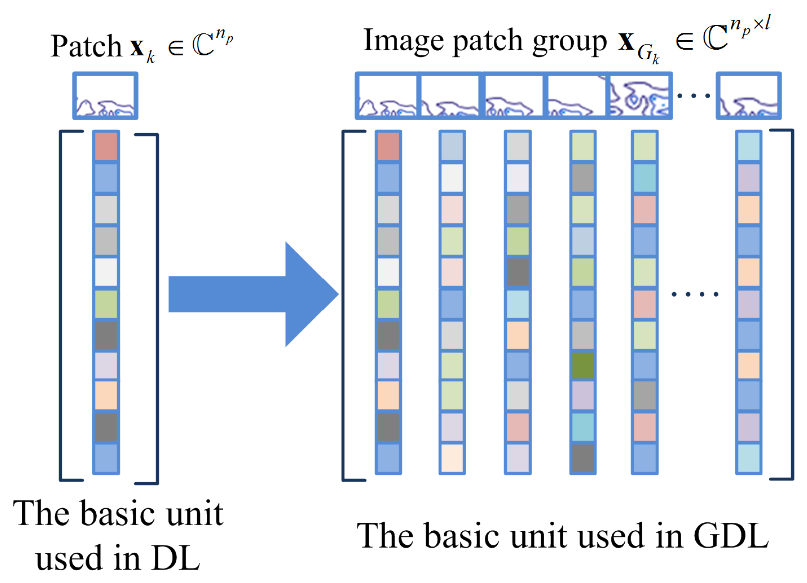
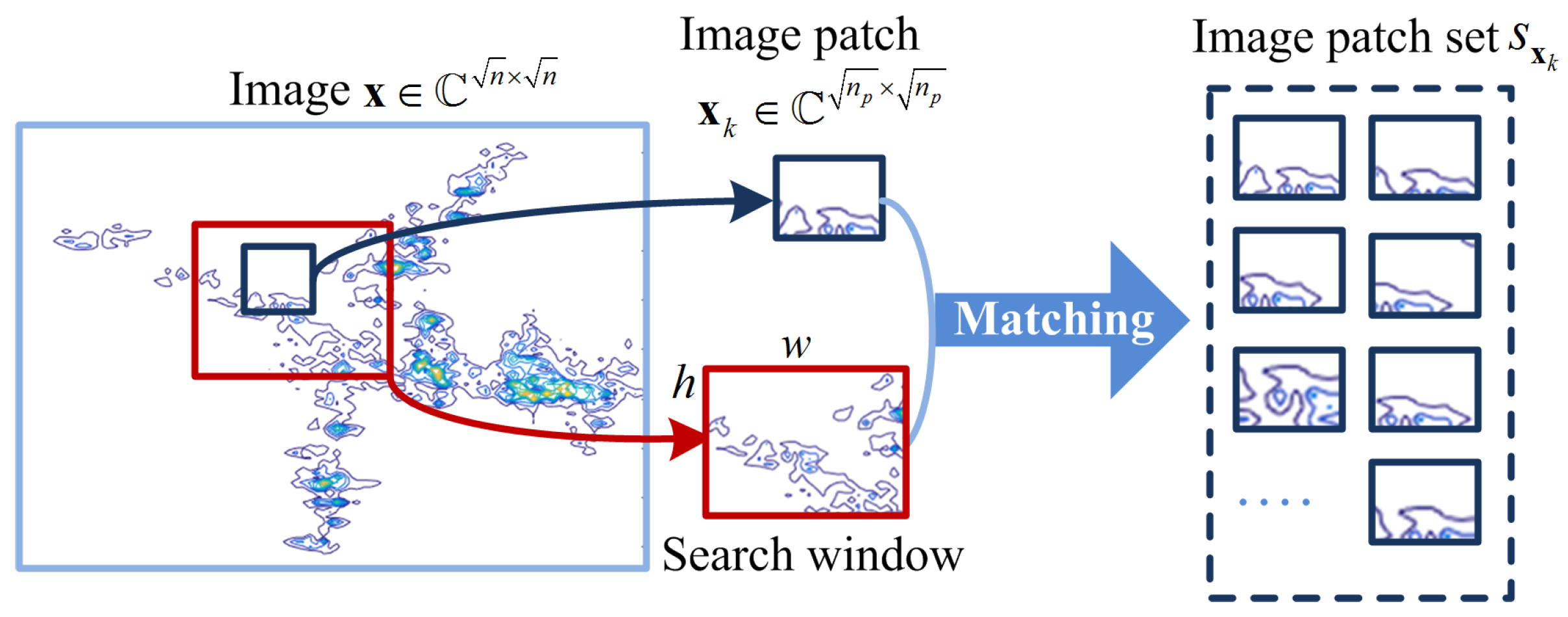
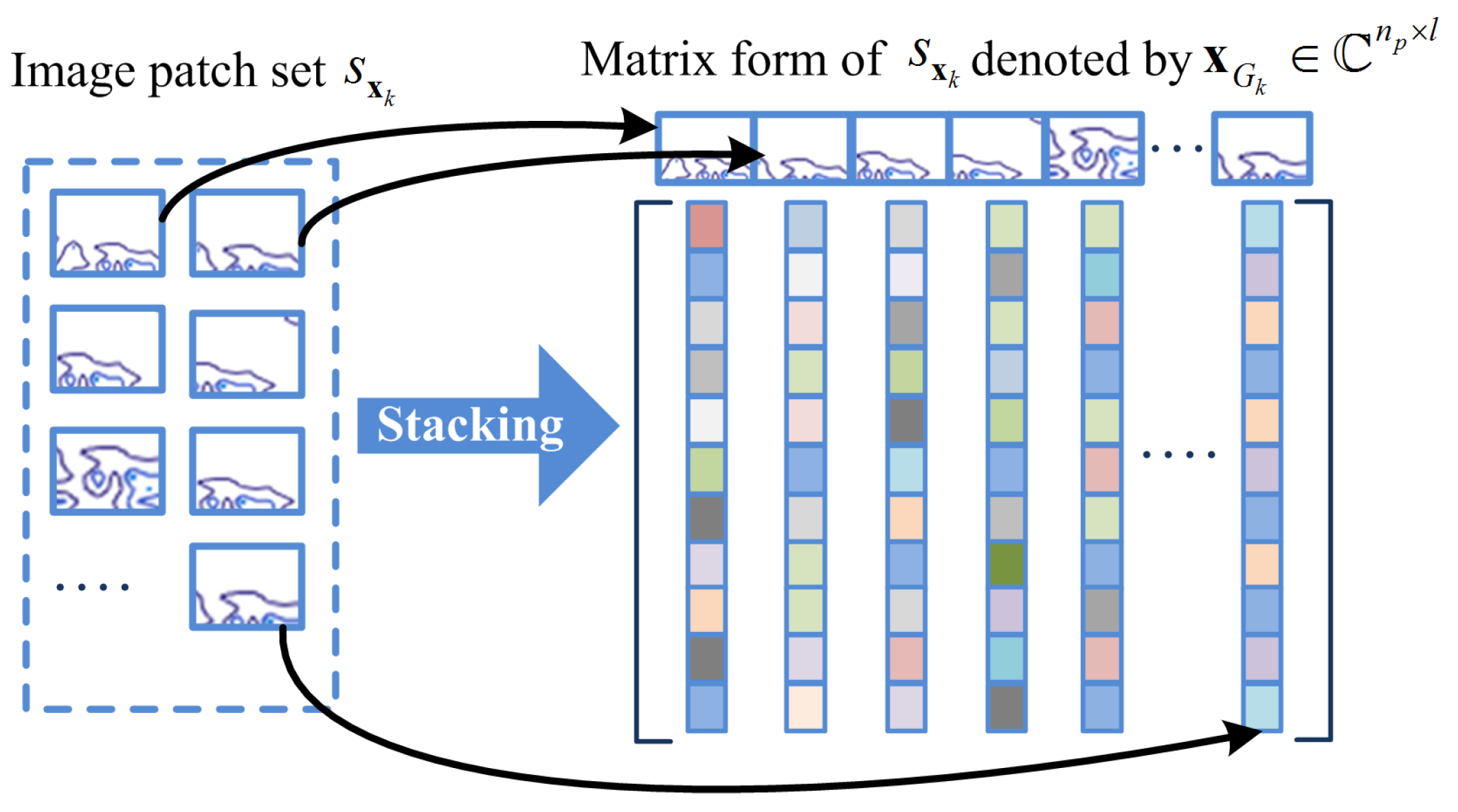
4.1. Construction of Image Patch Group

Given a vectorized image x , the size of x equals that of σ , i.e., x C n . In order to intelligibly elaborate the construction of IPG, the vectorized form of the x needs to be converted to the matrix form with the size of n × n as shown in Figure 1.
The image x is divided into N overlapped patches { x k } k = 1 N . For each patch x k C n p × n p , denoted by the dark blue square in Figure 1, in the search window (red square), we search its l best matched patches to compose the image patch set s x k . Here, the similarity between patches is measured, using a certain similarity criterion.
Next, all the patches in s x k are stacked into a matrix of size n p × l , represented by x G k , which contains every patch in s x k as its columns, as shown in Figure 2. The matrix x G k , including all patches with similar structures, is named an IPG. For simplicity, we define the construction of the IPG as follows:
x G k = F G k ( x )
where F G k ( · ) denotes the operator that extracts the k t h IPG from x , and its transpose, denoted by F G k T ( · ) , can put the k t h IPG back into its original position in the reconstructed image, padded with zeros elsewhere.
By averaging all the IPGs, the reconstruction of the whole image x from set { x G k } k = 1 N becomes the following:
x ^ = k = 1 N F G k T ( x G k ) . / k = 1 N F G k T ( B )
where . / " denotes the element-wise division and B is a matrix of size n p × l with all the elements being 1.
Note that in our work, each patch x k is represented as a vector, and each IPG x G k is represented as a matrix as shown in Figure 3. According to the above definition, it is obvious to observe that each patch x k corresponds to an IPG x G k . One can also see that the construction of x G k explicitly exploits the self-similarity information between patches.

4.2. ISAR Image Patch Group Based Imaging Model

Let I be an initial ISAR target image obtained by directly implementing the 2D FFT on the measurements G s , represented by the following:
I = Ψ T G s
The quality of the initial target image I C n is very poor as expected since the pulses cannot be coherently integrated. The purpose of GDL-based imaging is to completely reconstruct the high quality target image σ from I .
According to the method provided in Section 4.1, we construct the ISAR IPG set { I G k } k = 1 N using the I , and the size of each I G k is n p × l . During the construction of each IPG, the cross-correlation is selected as the criterion to measure the similarity between patches. Thus, reconstructing the σ from I can be modeled as follows:
min σ k = 1 N I G k 1 s . t . G s Ψ σ 2 2 < ϵ

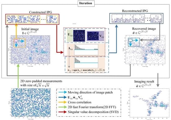
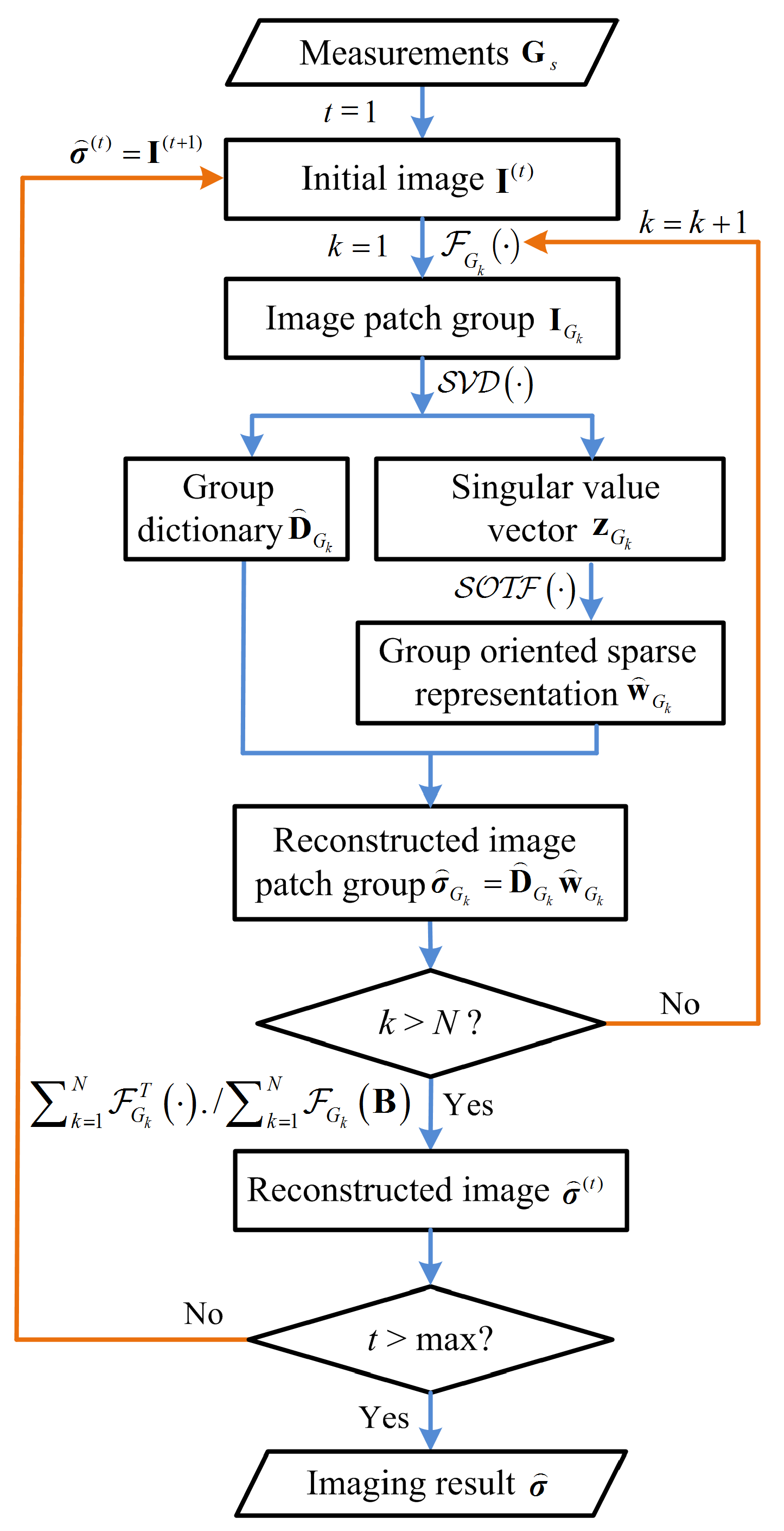
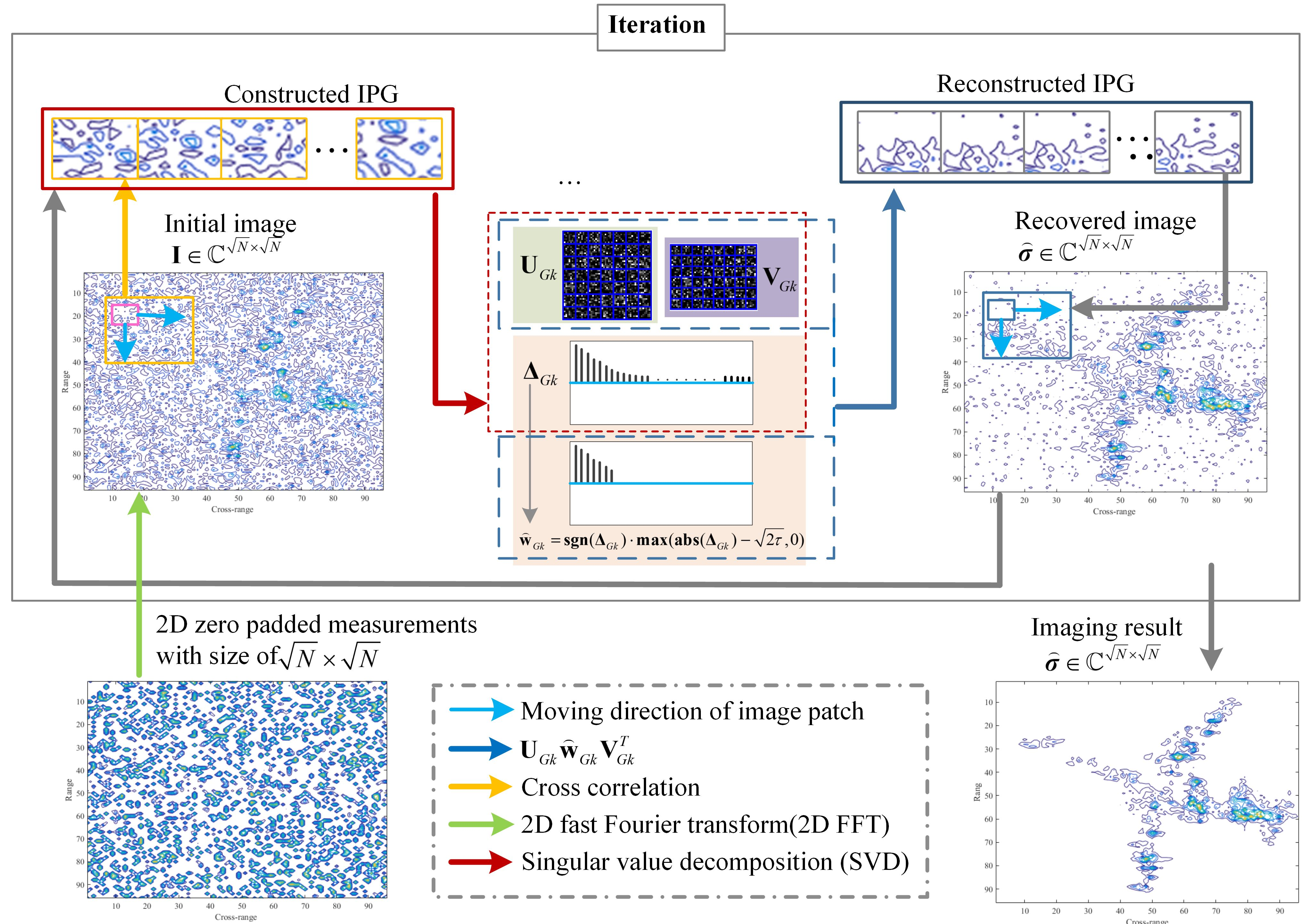
4.3. Group Dictionary Learning Based Sparse Imaging

To enforce the local sparsity and the self-similarity of target image simultaneously in a unified framework, we suppose that the I G k can be sparsely represented over a group dictionary D G k . Here, D G k = { d ( G k , 1 ) , d ( G k , 2 ) , , d ( G k , m ) } is assumed to be known. Note that each atom d ( G k , i ) C n p × l is a matrix of the same size as the IPG I G k , and m is the number of atoms in D G k . Different from the dictionary in patch-based DL, here, D G k is of size ( n p × l ) × m , that is, D G k C ( n p × l ) × m . How to learn D G k with high efficiency is given in detail in the next subsection.
Similar to the notations about sparse coding process in patch-based DL, the sparse coding process of each IPG over D G k is to seek a sparse representation w G k C m such that I G k D G k w G k , we refer to the w G k as GOSR. Thus, the target image reconstruction model in Equation (15) can be rewritten as follows:
min σ k = 1 N w G k 1 s . t . G s Ψ σ 2 2 < ϵ
Only measurement G s and IPG set { I G k } are available. However, we need to obtain the optimal group dictionaries { D G k } k = 1 N and corresponding GOSRs { w G k } k = 1 N . Similar to the joint optimization model in on-line DL-based sparse imaging described in Section 3, we reform the reconstruction model in Equation (16) as a joint optimization model as follows:
min σ , { D G k } , { w G k } k = 1 N I G k D G k w G k 2 2 + μ G s Ψ σ 2 2 s . t . k w G k 1 T g
where T g is sparse level of each group. The weight μ in our formulation is a positive constant and balances the measurements fidelity and GOSRs. The first term in Equation (17) captures the quality of the sparse approximations of { I G k } with respect to group dictionaries { D G k } , the second term in the cost measures of the measurements fidelity.
Our formulation is, thus, capable of designing an adaptive group dictionary for each IPG, and also using the group dictionary to reconstruct the current IPG. In addition, the model in Equation (17) can typically avoid artifacts seen in the initial image obtained in Section 4.2. All of the above are done, using only the under-sampled measurements G s and set { I G k } .
In our work, we adopt the alternate iteration strategy to minimize the joint optimization problem in Equation (17) to solve the { D G k } , the { w G k } and the σ . Each iteration includes N cycles, and each cycle involves two steps: learning D G k as well as jointly optimizing the w G k and I G k . In the first step, D G k is obtained by GDL, while the corresponding I G k and w G k are fixed. In the second step, the learned D G k is fixed, w G k and I G k are estimated by solving a l 1 norm minimization problem. The details of these two steps are further given in the following subsections.

4.4. Group Dictionary Learning

In this subsection, we show how to learn the group dictionary D G k for each IPG I G k . Note that, on one hand, we hope that each I G k can be represented by the corresponding D G k faithfully. On the other hand, we hope that the sparse representation coefficient of I G k over the D G k is as sparse as possible. According to the patch-based DL method presented in Section 3, the GDL can be intuitively modeled as follows:
min { D G k } k = 1 N I G k D G k w G k 2 2 s . t . k w G k 1 T g
Note that the group dictionary form is very complex. If we adopt the iteration method, such as K-SVD, to learn group dictionary, it is a time-consuming process. Therefore, we do not directly utilize Equation (18) to learn the group dictionary for each IPG.
In order to obtain the group dictionary with high efficiency, in this paper, the SVD-based GDL method is directly performed on each I G k . Thus, the I G k can be decomposed into the sum of a series of weighted rank-one matrices as follows:
SVD ( I G k ) = U G k Δ G k V G k H = i = 1 m δ ( G k , i ) ( u ( G k , i ) v ( G k , i ) H )
where Δ G k = { δ ( G k , 1 ) , δ ( G k , 2 ) , , δ ( G k , m ) } is the singular value set, z G k C m denotes the singular value vector with the values in set Δ G k as its elements. The left singular vector u ( G k , i ) C n p and the right singular vector v ( G k , i ) C l are the columns of unitary matrices U G k C n p × n p and V G k C l × l , respectively. H represents the Hermitian transpose operation.
Each atom in D G k for I G k is defined as follows:
d ( G k , i ) = u ( G k , i ) v ( G k , i ) H
where the d ( G k , i ) C n p × l .
Therefore, the ultimate adaptively learned group dictionary for I G k is defined as follows:
D ^ G k = { d ( G k , 1 ) , d ( G k , 2 ) , , d ( G k , m ) }
Based on the definitions in above, we can obtain I G k = D G k z G k . From Equations (19)–(21), we can obviously see that the SVD-based GDL method guarantees that all the patches in an IPG use the same group dictionary and share the same dictionary atoms. In addition, it is clear to see that the proposed GDL is self-adaptive to each IPG I G k and is quite efficient, requiring only one SVD for each IPG.

4.5. Group Sparse Representation and Target Image Reconstruction

According to the second term in Equation (17), the joint optimization problem of GOSRs and the target image can be formulated as follows:
min σ , { w G k } k = 1 N μ G s Ψ σ 2 2 s . t . k w G k 1 T g
By multiplying the Ψ T for G s and Ψ σ , the Equation (22) becomes the following:
min σ , { w G k } k = 1 N μ σ I 2 2 s . t . k w G k 1 T g
where σ denotes the target image to be reconstructed and I is the initial image of σ defined in Section 4.2.
The Equation (23) can be rewritten as a regularized form by introducing a regularized parameter λ :
{ σ ^ , { w ^ G k } } = min σ , { w G k } σ I 2 2 + λ μ k = 1 N w G k 1
where the parameter λ / μ controls the trade-off between the first and second terms in Equation (24).
The Equation (24) can be minimized in the iteration manners of greedy pursuit or convex optimization. In each iteration, using the I to reconstruct the σ , the reconstructed σ is regarded as a novel I in next iteration. Since the form of the k = 1 N w G k 1 is too complicated, to exactly reconstruct σ from I in the iteration manners is a very hard process.
In order to reduce the difficulty of minimizing Equation (24), we perform some experiments to investigate the statistics of the error between the initial images I ( t ) and corresponding reconstruction results σ ( t ) in each iteration, where t is the index of iteration. Since obtaining the initial images and the exact reconstruction results is not available, we use the poor quality images obtained by the RD method with different under-sampled measurements to approximate the initial images and reconstructed results. Concretely, the images reconstructed with 25%, 30% and 35% measurements are regarded as the approximated initial images in 1st, 2nd and 3rd iterations, and the images obtained by 30%, 35% and 40% measurements are regarded as the reconstruction result in the 1st, 2nd and 3rd iterations.
We use the real plane data and ship data as the examples. By implementing the approximate operation mentioned above for the motion compensated real plane data, we can calculate the reconstruction errors e ( t ) = σ ( t ) I ( t ) in the first three iterations, i.e., t = 1 , 2 , 3 . Then, we can drawn the probability density histograms for e ( 1 ) , e ( 2 ) and e ( 3 ) , as shown in Figure 4a–c, respectively. In Figure 4a, the horizontal axis denotes the range of the pixel values in error matrix e ( 1 ) , and the vertical axis denotes the probability of the number of pixel values in different ranges to the number of total pixel. From Figure 4a, we can observe that the probability density histograms of e ( 1 ) can quite be characterized as a generalized Gaussian distribution (the probability density function of generalized Gaussian distribution is given in https://sccn.ucsd.edu/wiki/Generalized_Gaussian_Probability_Density_Function, accessed on 22 November 2020.) where the mean is zero and variance is v ( t ) . The v ( t ) is estimated by the following:
v ( t ) = 1 n σ ( t ) I ( t ) 2 2
where n is the number of total pixels.
Similar to observation in Figure 4a, the probability density histograms of e ( 2 ) and e ( 3 ) shown in Figure 4b,c can also be approximated as the generalized Gaussian distributions.
We also perform the approximation operation mentioned above for the motion compensated ship data. The probability density histograms of e ( 1 ) , e ( 2 ) and e ( 3 ) of ship data are shown in Figure 4d–f, which have distributions similar to those of the plane data.
Based on the statistics of the probability density histograms of reconstruction errors in the iteration process, to enable minimizing Equation (24) tractably, a reasonable assumption is made in this paper. We suppose that each element in e ( t ) satisfies an independent distribution with zero mean and variance be v ( t ) . By this assumption, for ε > 0 , we can obtain the following conclusion:
lim n K P { | 1 n σ I 2 2 1 K k = 1 N σ G k I G k 2 2 | < ε } = 1
where σ G k denotes the to be reconstructed IPG, P ( · ) be a probability function. Probability coefficient K = n p × l × N with n p is the size of the patch, l is the number of patches in an IPG, and N is the number of IPGs extracted from the initial image. The detailed proof of Equation (26) is given in Appendix A.
According to the approximation in Equation (26), we have the following equation with probability nearly at 1:
σ I 2 2 = n K k = 1 N σ G k I G k 2 2
Incorporating Equations (27)–(24), we have the following:
min σ , { w G k } σ I 2 2 + λ μ k = 1 N w G k 1 = min σ , { w G k } n K k = 1 N σ G k I G k 2 2 + λ μ k = 1 N w G k 1 = min σ , { w G k } k = 1 N { σ G k I G k 2 2 + η w G k 1 }
where η = λ K / μ n .
Note that (28) can be efficiently minimized by solving N joint optimization problems, each of which is expressed as follows:
{ σ ^ G k , w ^ G k } = min σ G k , w G k σ G k I G k 2 2 + η w G k 1
From the definitions of w G k , z G k we can know σ G k = D G k w G k and I G k = D G k z G k , z G k is the singular value vector defined in Section 4.4. Due to the construction of D G k in Equation (21) and the unitary property of U G k and V G k , we can obtain the following relationship:
σ G k I G k 2 2 = w G k z G k 2 2
The detailed proof of Equation (30) is provided in Appendix B.
Submitting Equation (30) into Equation (29), Equation (29) can then be minimized by solving w G k first:
w ^ G k = min w G k w G k z G k 2 2 + η w G k 1
According to Lemma 1 in [25], the closed-form solution of w G k is as follows:
w ^ G k = SOTF ( z G k , η ) = sgn ( z G k ) · max ( abs ( z G k ) η , 0 )
where SOTF ( · ) denotes the soft thresholding function and “·” denotes the element-wise product.
Then, the IPG in Equation (29) can be reconstructed by the following:
σ ^ G k = D ^ G k w ^ G k
where D ^ G k is the group dictionary obtained in Equation (21).
According to the strategy of alternatively solving Equations (21) and (29), all IPGs can be sequentially recovered, and the target image is reconstructed through Equation (13).
So far, all issues in the process from under-sampled measurements to the target image reconstruction have been solved. In light of all derivations above, a detailed flow chart of the proposed algorithm for ISAR imaging using GDL is shown in Figure 5.

5. Experimental Results

In this section, we use real plane data and ship data sets to demonstrate the performance of the proposed GDL based ISAR imaging method. In order to evaluate the feasibility and the chief advantages of our method faithfully, the GDL ISAR imaging method is compared with the greedy Kalman filtering (GKF) imaging method [9], ISAR image patch based online dictionary learning (ONDL) imaging method and offline dictionary learning (OFDL) imaging method [15], which deal with the ISAR data in a spatial domain and transform domain adaptive to ISAR data, respectively.

5.1. Imaging Data and Parameters

The plane data were collected by a ground-based ISAR operating at C band; the bandwidth of the transmitted waveform is 400 MHz. A de-chirp processing was used for the range compression of the plane data. The ship data were collected by a shore-based X-band radar, and the bandwidth of corresponding transmitted waveform is 80 MHz.
All data sets were motion compensated by the minimum entropy based global range alignment algorithm [26] as well as the improved phase gradient algorithm (PGA) [27]. The details of the size of the raw data ( S_r_data ), under-sampling ratios ( S_ratios ) as well as the sparsity are listed in Table 1. Note that the sparsity is estimated, using the approach in [28].
All data sets used for verifying the reconstruction performance of the proposed imaging method were obtained by performing a random under-sampling operation on both the range domain and cross-range domain of the corresponding motion-compensated raw data. For the plane data, we consider two types of under-sampling ratios, which are 25 % and 50 % . For the ship data, we set the under-sampling ratio to 50 % , i.e., 4608 measurements, as listed in Table 1.
We set the optimal parameters in the GDL-based imaging method as listed in Table 2. The detailed settings of all the parameters are discussed in Section 5.5. All the experiments are performed in Matlab2015b on an assembled computer with Intel (R) Core (TM) i7-7700 CPU @ 3.60 GHz, 8G memory, and a Windows 7 operating system.

5.2. Image Quality Evaluation

To provide a quantitative evaluation of the images reconstructed with the proposed imaging method, we use two types of performance evaluation indices [29]. One is the “true-value” based indices and the other is the conventional image quality indices. The “true-value” based indices assess the accuracy of position of reconstructed scatterers. The conventional indices mainly assess the visual quality of the reconstructed images.
The “true-value” based evaluation is based on the comparison of the original or reference image (which represents the “true-value”) with the reconstructed image. Since we do not have ground-truth images of non-cooperative targets, in our experiment, a high-quality image reconstructed by the conventional RD method using full data is referred to as the reference image in our work. Thus, the metrics evaluate the performance of the proposed GDL-based imaging method as compared to the RD method. The “true-value” based evaluation uses the following indices: False Alarm (FA) and Missed Detection (MD). FA is used for assessing the scatterers that are incorrectly reconstructed. MD is used for assessing the missed scatterers.
The conventional image quality evaluation includes the target-to-clutter ratio (TCR), image entropy (ENT) and image contrast (IC). The TCR that we use in our work is defined as follows:
TCR = 10 log 10 ( r , p ) Ω τ σ ^ ( c , r ) 2 ( c , r ) Ω c σ ^ ( c , r ) 2
where ( c , r ) represents the pixel index, σ ^ ( c , r ) denotes the reconstructed value at pixel ( c , r ) in the reconstructed image σ ^ and Ω τ , Ω c denote the target region and clutter region in σ ^ , respectively. We determine Ω τ and Ω c by performing a binarization processing on the RD image. The pixels whose values are greater than a specified threshold are classified into Ω τ and otherwise into Ω c .

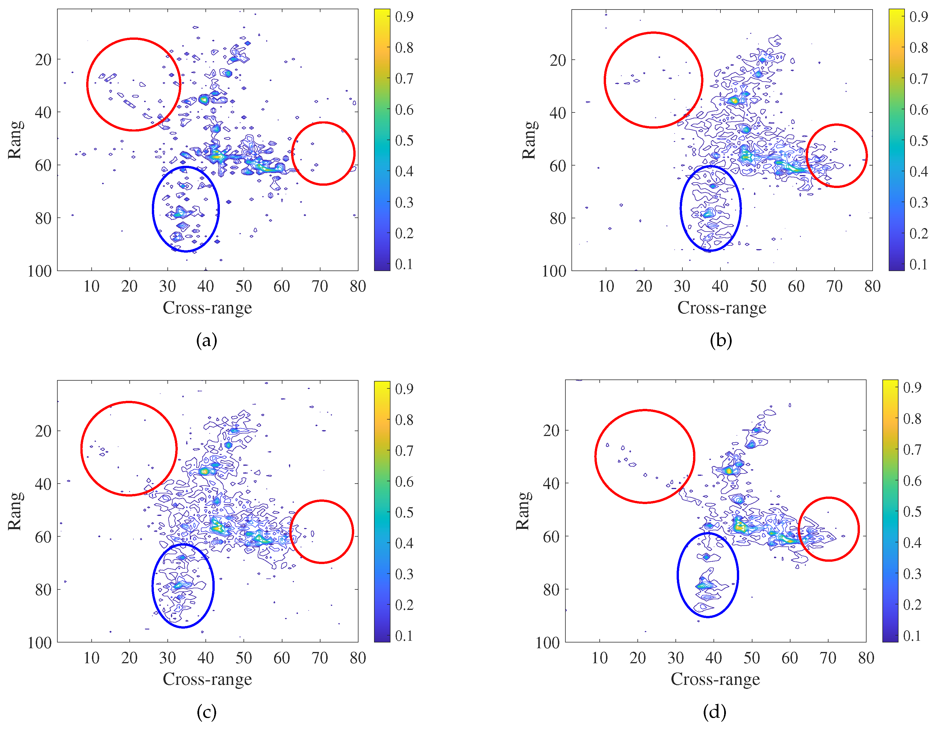
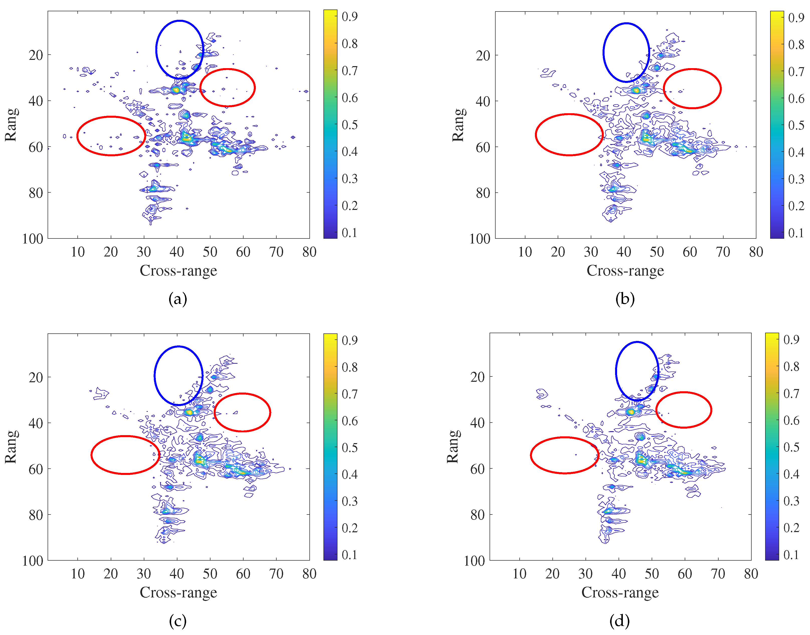
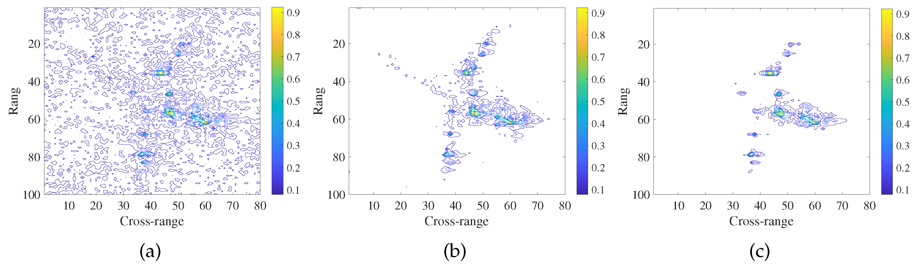
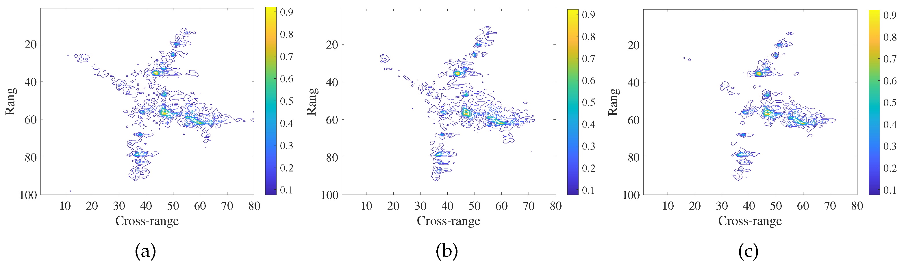
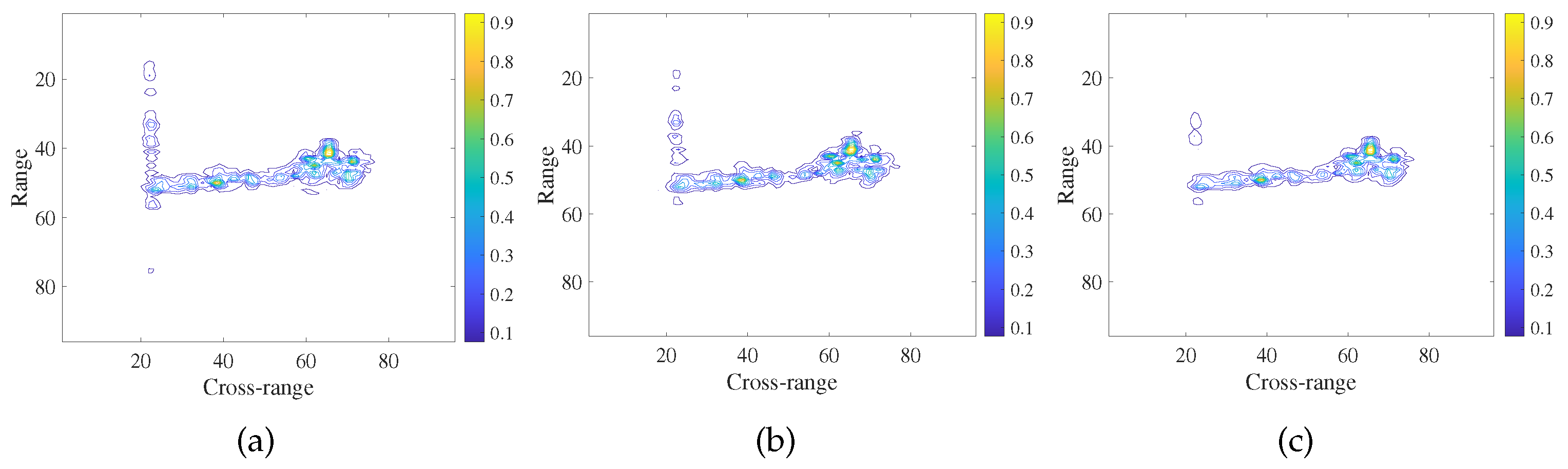
5.3. Imaging Results of Real Data

Figure 6a,b presents the full data imaging results of the plane data and ship data, using the RD method, respectively.
Figure 7 shows the imaging results of 25% measurements of plane data, using the GKF, ONDL, and OFDL, as well as our GDL-imaging methods, respectively. Figure 8 shows the imaging results of 50% measurements of plane data. Figure 9 shows the imaging results obtained by 50 % ship raw data, using the different imaging methods mentioned above. Note that all imaging results are displayed with the same contour level.
Comparing Figure 7a–d, we see that many artifacts appear in the results of the GKF, ONDL, and OFDL methods. The first three imaging methods cannot provide well-reconstructed images, while our GDL method well reconstructs the nose, tail, and wings of the plane as indicated by the red and blue circles in Figure 7. This verifies the superiority of the proposed GDL-based imaging method in target shape reconstruction. The GOSR obtained by the group dictionary can account for the self-similarity information between image patches, leading to better retaining of the information regarding the plane shape as compared to the other methods considered here.
Figure 8 shows the imaging results of 50% measurements of plane data, using the imaging methods considered here. Specifically, the GDL-based imaging method provides the best results. The fewest artifacts appear in the reconstructed image of GDL as shown in the regions indicated by the red and blue circles in Figure 8.
From Figure 9 we can see that the ship target can be reconstructed successfully, using these four methods. It shows the imaging results of the ship target obtained by the GKF, ONDL, OFDL, and GDL methods, using 50% measurements. By performing a further comparison of the regions indicated by red circles and blue rectangles, we see that the result shown in Figure 9d have the fewest artifacts or interferences.
We also see that there are some errors in the results of the GDL method, for example, the poor reconstruction of the nose of the plane in Figure 7. Note that the target region is reconstructed exploiting GOSRs that are calculated with Equation (32), which reflects that the quality of the GOSRs is influenced by the singular value vector of IPG and the soft thresholding. Therefore, the reasons for the poor reconstruction of the target may be that the singular value vector of IPG or the soft thresholding are not accurate enough.

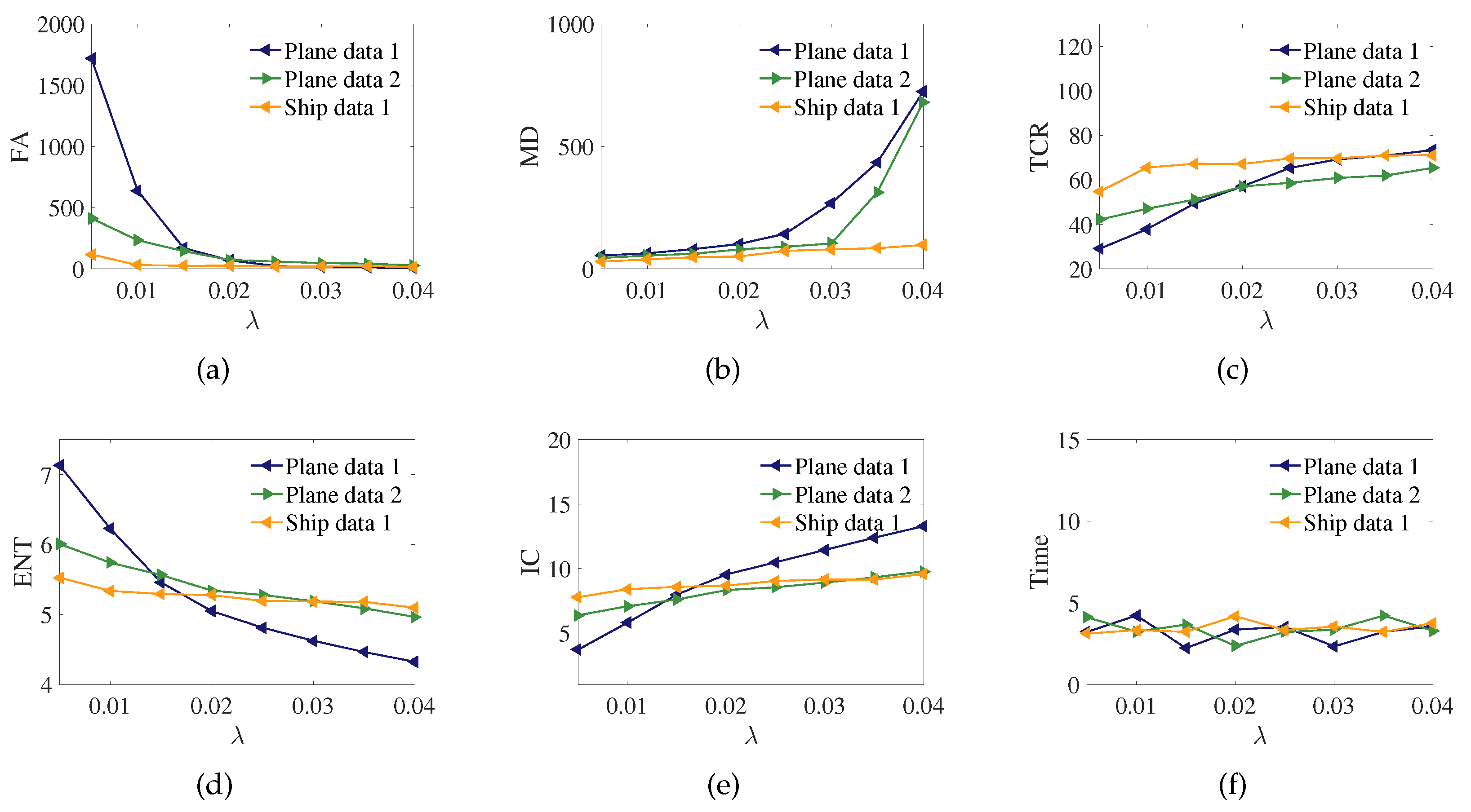
5.4. Quantitative Evaluation of Image Quality

Except for the visual comparisons of the imaging results, we also evaluate the image quality using the metrics introduced in Section 5.2. The evaluations of the imaging results are listed in Table 3.
From the second and third columns in Table 3, we see the results of our method have the smallest FA and MD, which means that our method can reconstruct the position of target scatterers most accurately and suppress the artifacts and sidelobe in the background well. This is consistent with the imaging results shown in Figure 7, Figure 8 and Figure 9.
As indicated in the fourth, fifth and sixth columns in Table 3, the TCR, ENT and IC of the GDL-based imaging method show the best values. This is also consistent with the visual comparison of Figure 7, Figure 8 and Figure 9.
The last column of Table 3 presents the computing time of each imaging method considered. It can be seen that the proposed GDL-based imaging method is the fastest one among all methods. This is due to the non-iterative processing employed in the SVD during the GDL process as compared to other methods.

5.5. Discussion on the Parameter Setting

In our experiments, all parameters in GDL based imaging method are shown in Table 2. The P _ s i z e denotes the size of the vectorized image patch, and the P _ s t e p denotes the moving step of the search window on the initial image during the IPG extraction process. h × w represents the initial size of search window, and l represents the number of similar image patches in an IPG. The μ and λ are the regularization parameters. The parameters, including P _ s i z e , P _ s t e p , h × w , l, μ and λ , are set empirically as shown in Table 2 and are kept unchanged for all three data sets where λ is adjustable.
From Equations (31) and (A1), we know the parameter λ balances the suppression of the artifacts and the preservation of the details of the target. If λ is too small, the artifacts cannot be fully suppressed, whereas if λ is too large, the target details may be lost. Thus, we consider the visual results and the quantitative indices of the imaging results simultaneously to explore the optimal values of λ for each type of imaging data.
Figure 10 shows the variation of FA, MD, TCR, ENT, IC and Times with different values of λ , where other parameters, including P _ s i z e , P _ s t e p , h × w , l, μ are kept constant for three data sets. We see that as the λ increases, the values of FA and ENT decrease, while the values of MD, TCR and IC increase. Note that all metrics but MD tend to the optimal situation with the increase in λ . The higher MD, in fact, indicates the sparser result, which means that the target structure details in the result may be missing, leading to the relatively bad appearance.
The target images of three data sets with different values of λ are shown in Figure 11, Figure 12 and Figure 13, respectively. From the Figure 11b, Figure 12b and Figure 13b; we can see that three data sets have the best image quality in the case of λ that equals 0.02, 0.03 and 0.035, respectively. The target images have the smallest number of artifacts and the best target shape. Furthermore, the quantitative indices of the three results are better than those of the results obtained by other imaging methods as shown in Table 3. Thus, the optimal values of λ for plane data 1 and plane data 2 as well as ship data 1 imaging can be set as 0.02, 0.03 and 0.035, respectively.

6. Conclusions

In this paper, we extended the DL-based ISAR sparse imaging method and presented the GDL based ISAR sparse imaging method. The GDL without the time-consuming iteration process has high efficiency. The sparse representation extracted from IPG contains the self-similarity information between the image patches and the local sparse prior information of the target image. The self-similarity information is very helpful in preserving the target shape or contour during the imaging process. The GDL ISAR sparse imaging method is better than the state-of-the-art ISAR sparse imaging methods considered in this paper in both imaging quality and computation speed.

Author Contributions

Conceptualization, C.H. and L.W.; methodology, C.H. and L.W.; software, C.H; validation, C.H. and L.W.; formal analysis, C.H.; writing—original draft preparation, C.H.; writing—review and editing, L.W., D.Z. and O.L.; visualization, C.H.; funding acquisition, L.W. All authors have read and agreed to the published version of the manuscript.

Funding

This work is supported by the National Key Research and Development Program of China with the Grant No. 2017YFB0502700, the National Natural Science Foundation of China with the Grant No. 61871217, the Aviation Science Foundation with the Grant No. 20182052011 and the Postgraduate Research and Practice Innovation Program of Jiangsu Province with the Grant No. KYCX18_0291, the Fundamental Research Funds for Central Universities under Grant NZ2020007 and the Fundamental Research Funds for Central Universities under Grant NG2020001.

Institutional Review Board Statement

Not applicable.

Informed Consent Statement

Not applicable.

Data Availability Statement

Data sharing is not applicable to this article.

Conflicts of Interest

The authors declare no conflict of interest.

Appendix A

Theorem A1.
Let σ C n × n , I C n × n , σ G k C n p × n p , I G k C n p × n p , be the error between σ and I denoted by e = σ I , where each element in e is represented by e i , i = 1 , , n . Assume that e i is independent and satisfies a distribution with N ( 0 , v 2 ) . Then, for ε > 0 , the relationship between σ I 2 2 and k = 1 N σ G k I G k satisfies the following property:
lim n K P { | 1 n σ I 2 2 1 K k = 1 N σ G k I G k 2 2 | < ε } = 1
Proof. 
Based on the assumption that each e i is independent, we know that each e i 2 is also independent. Since mean E { e i } = 0 and variance V { e i } = v 2 , the mean of e i 2 can be expressed as follows:
E { e i 2 } = V { e i } + { E { e i } } 2 = v 2
By invoking the Convergence in Probability of Law of Large Numbers, for ε > 0 , it leads to the following:
lim n P { | 1 n i = 1 n e i 2 v 2 | < ε 2 } = 1
i.e.,
lim n P { | 1 n σ I 2 2 v 2 | < ε 2 } = 1
Further, let σ G and I G denote the concatenations of all σ G k and I G k , respectively. The error between σ G and I G is represented by e G where each element in e G denoted by e j , j = 1 , 2 , , K and K = n p × l × N . Due to the assumption that each e j is independent and satisfies a distribution with N ( 0 , v 2 ) , the same manipulation with Equation (A3) applied to e j 2 yields the following:
lim K P { | 1 K j = 1 K e j 2 v 2 | < ε 2 } = 1
which can be rewritten as follows:
lim K P { | 1 K k = 1 N σ G k I G k 2 2 v 2 | < ε 2 } = 1
From Equation (A4), we know the following:
lim n P { ε 2 < ( 1 n σ I 2 2 v 2 ) < ε 2 } = 1 lim n P { ε 2 < ( 1 n σ I 2 2 1 K k = 1 N σ G k I G k 2 2 ) + ( 1 K k = 1 N σ G k I G k 2 2 v 2 ) = β < ε 2 } = 1 lim n P { ε 2 β < 1 n σ I 2 2 1 K k = 1 N σ G k I G k 2 2 < ε 2 β } = 1
From Equation (A6) we know lim K P { β ( ε 2 , ε 2 ) } = 1 . Therefore, when K , we have ε 2 β > ε 2 ( ε 2 ) = ε and ε 2 β < ε 2 ( ε 2 ) = ε . Thus, the Equation (A7) can be scaled to the following:
lim n K P { ε < 1 n σ I 2 2 1 K k = 1 N σ G k I G k 2 2 < ε } = 1
i.e.,
lim n K P { | 1 n σ I 2 2 1 K k = 1 N σ G k I G k 2 2 | < ε } = 1
Therefore, the Equation (A1) is proved.  □

Appendix B

Theorem A2.
σ G k I G k 2 2 = w G k z G k 2 2
Proof. 
According to the definitions of D G k , w G k and z G k , we have the following:
σ G k = D G k w G k I G k = D G k z G k
Then,
σ G k I G k 2 2 = D G k w G k D G k z G k 2 2 = U G k diag ( w G k ) V G k H U G k diag ( z G k ) V G k H 2 2 = U G k diag ( w G k z G k ) V G k H 2 2
where diag ( · ) denotes the diagonal matrix.
According to the property that the square of F norm of a matrix equals its trace, the Equation (A12) can be unfolded as follows:
U G k diag ( w G k z G k ) V G k H 2 2 = T ( U G k diag ( w G k z G k ) V G k H ( U G k diag ( w G k z G k ) V G k H ) H ) = T ( U G k diag ( w G k z G k ) V G k H V G k = V G k 1 V G k = E diag ( w G k z G k ) U G k H ) = T ( U G k diag ( w G k z G k ) diag ( w G k z G k ) U G k H ) = T ( diag ( w G k z G k ) U G k U G k H diag ( w G k z G k ) ) = T ( diag ( w G k z G k ) diag ( w G k z G k ) ) = w G k z G k 2 2
where T ( · ) is the operator for calculating the trace of a matrix.  □

References

  1. Chen, V.C.; Martorella, M. Principles of Inverse Synthetic Aperture Radar SAR Imaging; Scitech: Raleigh, NC, USA, 2014. [Google Scholar]
  2. Cetin, M.; Karl, W.C. Feature-enhanced synthetic aperture radar image formation based on nonquadratic regularization. IEEE Trans. Image Process. 2001, 10, 623–631. [Google Scholar] [CrossRef] [PubMed] [Green Version]
  3. Cetin, M.; Karl, W.C.; Castanon, D.A. Feature enhancement and ATR performance using nonquadratic optimization-based SAR imaging. IEEE Trans. Aerosp. Electron. Syst. 2003, 39, 1375–1395. [Google Scholar]
  4. Zhang, X.; Bai, T.; Meng, H.; Chen, J. Compressive Sensing-Based ISAR Imaging via the Combination of the Sparsity and Nonlocal Total Variation. IEEE Geosci. Remote Sens. Lett. 2014, 11, 990–994. [Google Scholar] [CrossRef]
  5. Xu, Z.; Wu, Y.; Zhang, B.; Wang, Y. Sparse radar imaging based on L1/2 regularization theory. Chin. Ence Bull. 2018, 63, 1306–1319. [Google Scholar] [CrossRef]
  6. Wang, M.; Yang, S.; Liu, Z.; Li, Z. Collaborative Compressive Radar Imaging With Saliency Priors. IEEE Trans. Geosci. Remote Sens. 2019, 57, 1245–1255. [Google Scholar] [CrossRef]
  7. Samadi, S.; Cetin, M.; Masnadi-Shirazi, M.A. Sparse representation-based synthetic aperture radar imaging. IET Radar Sonar Navig. 2011, 5, 182–193. [Google Scholar] [CrossRef] [Green Version]
  8. Raj, R.G.; Lipps, R.; Bottoms, A.M. Sparsity-based image reconstruction techniques for ISAR imaging. In Proceedings of the 2014 IEEE Radar Conference, Cincinnati, OH, USA, 19–23 May 2014; pp. 0974–0979. [Google Scholar] [CrossRef]
  9. Wang, L.; Loffeld, O.; Ma, K.; Qian, Y. Sparse ISAR imaging using a greedy Kalman filtering. Signal Process. 2017, 138, 1. [Google Scholar] [CrossRef]
  10. Aharon, M.; Elad, M.; Bruckstein, A. K-SVD: An Algorithm for Designing Overcomplete Dictionaries for Sparse Representation. IEEE Trans. Signal Process. 2006, 54, 4311–4322. [Google Scholar] [CrossRef]
  11. Rubinstein, R.; Peleg, T.; Elad, M. Analysis K-SVD: A Dictionary-Learning Algorithm for the Analysis Sparse Model. IEEE Trans. Signal Process. 2013, 61, 661–677. [Google Scholar] [CrossRef] [Green Version]
  12. Ojha, C.; Fusco, A.; Pinto, I.M. Interferometric SAR Phase Denoising Using Proximity-Based K-SVD Technique. Sensors 2019, 19, 2684. [Google Scholar] [CrossRef] [PubMed] [Green Version]
  13. Chen, S.S.; Donoho, D.L.; Saunders, M.A. Atomic decomposition by basis pursuit. SIAM Review 2001, 43, 129–159. [Google Scholar] [CrossRef] [Green Version]
  14. Soğanlui, A.; Cetin, M. Dictionary learning for sparsity-driven SAR image reconstruction. In Proceedings of the 2014 IEEE International Conference on Image Processing (ICIP), Paris, France, 27–30 October 2014; pp. 1693–1697. [Google Scholar] [CrossRef]
  15. Hu, C.; Wang, L.; Loffeld, O. Inverse synthetic aperture radar imaging exploiting dictionary learning. In Proceedings of the 2018 IEEE Radar Conference (RadarConf18), Oklahoma City, OK, USA, 23–27 April 2018; pp. 1084–1088. [Google Scholar] [CrossRef]
  16. Kindermann, S.; Osher, S.; Jones, P.W. Deblurring and Denoising of Images by Nonlocal Functionals. Multiscale Model. Simul. 2005, 4, 1091–1115. [Google Scholar] [CrossRef]
  17. Elmoataz, A.; Lezoray, O.; Bougleux, S. Nonlocal Discrete Regularization on Weighted Graphs: A Framework for Image and Manifold Processing. IEEE Trans. Image Process. 2008, 17, 1047–1060. [Google Scholar] [CrossRef] [PubMed] [Green Version]
  18. Peyré, G. Image Processing with Nonlocal Spectral Bases. Multiscale Model. Simul. 2008, 7, 703–730. [Google Scholar] [CrossRef] [Green Version]
  19. Jung, M.; Bresson, X.; Chan, T.F.; Vese, L.A. Nonlocal Mumford-Shah Regularizers for Color Image Restoration. IEEE Trans. Image Process. 2011, 20, 1583–1598. [Google Scholar] [CrossRef] [PubMed] [Green Version]
  20. Zhang, J.; Zhao, D.; Jiang, F.; Gao, W. Structural Group Sparse Representation for Image Compressive Sensing Recovery. In Proceedings of the 2013 Data Compression Conference, Snowbird, UT, USA, 20–22 March 2013; pp. 331–340. [Google Scholar] [CrossRef]
  21. Varanasi, M.K.; Aazhang, B. Parametric generalized Gaussian density estimation. J. Acoust. Soc. Am. 1989, 86, 1404–1415. [Google Scholar] [CrossRef]
  22. Hu, C.; Wang, L.; Sun, L.; Loffeld, O. Inverse Synthetic Aperture Radar Imaging Using Group Based Dictionary Learning. In Proceedings of the 2018 China International SAR Symposium (CISS), Shanghai, China, 10–12 October 2018; pp. 1–5. [Google Scholar]
  23. Lazarov, A.; Minchev, C. ISAR geometry, signal model, and image processing algorithms. IET Radar Sonar Navig. 2017, 11, 1425–1434. [Google Scholar] [CrossRef]
  24. Tran, H.T.; Giusti, E.; Martorella, M.; Salvetti, F.; Ng, B.W.H.; Phan, A. Estimation of the total rotational velocity of a non-cooperative target using a 3D InISAR system. In Proceedings of the 2015 IEEE Radar Conference (RadarCon), Arlington, VA, USA, 10–15 May 2015; pp. 0937–0941. [Google Scholar] [CrossRef]
  25. Zhang, J.; Zhao, D.; Zhao, C.; Xiong, R.; Ma, S.; Gao, W. Image Compressive Sensing Recovery via Collaborative Sparsity. IEEE J. Emerg. Sel. Top. Circuits Syst. 2012, 2, 380–391. [Google Scholar] [CrossRef]
  26. Zhu, D.; Wang, L.; Yu, Y.; Tao, Q.; Zhu, Z. Robust ISAR Range Alignment via Minimizing the Entropy of the Average Range Profile. IEEE Geosci. Remote Sens. Lett. 2009, 6, 204–208. [Google Scholar] [CrossRef]
  27. Ling, W.; Dai, Y.Z.; Zhao, D.Z. Study on Ship Imaging Using SAR Real Data. J. Electron. Inf. Technol. 2007, 29, 401. [Google Scholar] [CrossRef]
  28. Wang, L.; Loffeld, O. ISAR imaging using a null space l1 minimizing Kalman filter approach. In Proceedings of the 2016 4th International Workshop on Compressed Sensing Theory and its Applications to Radar, Sonar and Remote Sensing (CoSeRa), Aachen, Germany, 19–22 September 2016; pp. 232–236. [Google Scholar] [CrossRef]
  29. Bacci, A.; Giusti, E.; Cataldo, D.; Tomei, S.; Martorella, M. ISAR resolution enhancement via compressive sensing: A comparison with state of the art SR techniques. In Proceedings of the 2016 4th International Workshop on Compressed Sensing Theory and Its Applications to Radar, Sonar and Remote Sensing (CoSeRa), Aachen, Germany, 19–22 September 2016; pp. 227–231. [Google Scholar] [CrossRef]
Figure 1. Extract each patch x k (as shown by the dark blue square) from image x and for each x k , search its l best similar patches in the search window (as shown by the red square) to compose the image patch set s x k .
Remotesensing 13 02812 g001
Figure 2. Reshape each patch in s x k to vector, and stack all vectors in the form of matrix to construct the image patch group x G k .
Remotesensing 13 02812 g002
Figure 3. The comparison between image patch x k and image patch group x G k .
Remotesensing 13 02812 g003
Figure 4. The probability density histograms of errors e ( t ) of the plane imaging in (a) t = 1, (b) t = 2 and (c) t = 3 iterations and the ship imaging in (d) t = 1, (e) t = 2 and (f) t = 3 iterations. The shape parameter ρ in generalized Gaussian probability density function keeps constant of 1.3 for these instances. The horizontal axis denotes the range of pixel values in e and the vertical axis denotes the probability G g d ( e ) of the number of pixel values in different ranges to the number of total pixels.
Remotesensing 13 02812 g004
Figure 5. The flow chart of the group dictionary learning based ISAR imaging algorithm.
Remotesensing 13 02812 g005
Figure 6. The (a) plane image and (b) ship image obtained by RD method using full data.
Remotesensing 13 02812 g006
Figure 7. The imaging results of the plane data obtained by (a) GKF imaging method, (b) ONDL imaging method, (c) OFDL imaging method and (d) the GDL imaging method, using 25% measurements.
Remotesensing 13 02812 g007
Figure 8. The imaging results of plane data obtained by (a) GKF imaging method, (b) ONDL imaging method, (c) OFDL imaging method and (d) the GDL imaging method, using 50% measurements.
Remotesensing 13 02812 g008
Figure 9. The target images of ship data yielded by (a) GKF imaging method, (b) ONDL imaging method, (c) OFDL imaging method as well as (d) the GDL imaging method using 50% measurements.
Remotesensing 13 02812 g009
Figure 10. The curves showing the variation of the quantitative indices (a) FA, (b) MD, (c) TCR, (d) ENT, (e) IC and (f) time of imaging quality with different values of λ for three data sets.
Remotesensing 13 02812 g010
Figure 11. The imaging results of 25% measurements of plane data reconstructed by GDL method in the three cases of (a) λ = 0.01, (b) λ = 0.02, and (c) λ = 0.03.
Remotesensing 13 02812 g011
Figure 12. The target images of 50% measurements of plane data obtained by GDL method in the three cases of (a) λ = 0.02, (b) λ = 0.03, and (c) λ = 0.04.
Remotesensing 13 02812 g012
Figure 13. The imaging results of 50% measurements of ship data yield by GDL method in the three cases of (a) λ = 0.02, (b) λ = 0.035, and (c) λ = 0.04.
Remotesensing 13 02812 g013
Table 1. The parameters of the real ISAR data sets used for verifying the performance of the GDL-based ISAR imaging method.
DataS_r_dataS_ratios (Measurements)Sparsity
Plane data100 × 8025% (2000), 50% (4000)900
Ship data96 × 9650% (4608)841
Table 2. The parameter settings of GDL imaging method for different ISAR data sets imaging.
DataP_sizeP_step h × w l μ λ
Plane data 164216 × 1664170.02
Plane data 264216 × 1664170.03
Ship data 164216 × 1664170.035
Table 3. Evaluation of real ISAR data image quality.
MethodsFAMDTCR(dB)ENTICTime(s)
GKF14420950.01795.32058.08501.3408 × 10 3
PlaneONDL17017348.65255.46747.72298.2370
data 1OFDL17313048.97755.55507.50455.9370
GDL7010257.12225.04829.53763.3620
GKF8613355.59305.38008.14491.221 × 10 3
PlaneONDL4518753.45935.31528.42997.2510
data 2OFDL5512559.97375.33958.38475.8510
GDL5210460.39725.25808.72783.3620
GKF8813256.31615.60367.59651.3301 × 10 3
ShipONDL15512653.62965.63887.32396.3620
data 1OFDL14815452.51805.71097.37724.3620
GDL205568.48285.18139.14544.1526
Publisher’s Note: MDPI stays neutral with regard to jurisdictional claims in published maps and institutional affiliations.

