


Abstract
Scanning radar enables wide-range imaging through antenna scanning and is widely used for radar warning. The Rayleigh criterion indicates that narrow beams of radar are required to improve the azimuth resolution. However, a narrower beam means a larger antenna aperture. In practical applications, due to platform limitations, the antenna aperture is limited, resulting in a low azimuth resolution. The conventional sparse super-resolution method (SSM) has been proposed for improving the azimuth resolution of scanning radar imaging and achieving superior performance. This method uses the norm to represent the sparse prior of the target and solves the regularization problem to achieve super-resolution imaging under the regularization framework. The resolution of strong-point targets is improved efficiently. However, for some targets with typical shapes, the strong sparsity of the norm treats them as strong-point targets, resulting in the loss of shape characteristics. Thus, we can only see the strong points in its processing results. However, in some applications that need to identify targets in detail, SSM can lead to false judgments. In this paper, a sparse denoising-based super-resolution method (SDBSM) is proposed to compensate for the deficiency of traditional SSM. The proposed SDBSM uses a sparse minimization scheme for denoising, which helps to reduce the influence of noise. Then, the super-resolution imaging is achieved by alternating iterative denoising and deconvolution. As the proposed SDBSM uses the norm for denoising rather than deconvolution, the strong sparsity constraint of the norm is reduced. Therefore, it can effectively preserve the shape of the target while improving the azimuth resolution. The performance of the proposed SDBSM was demonstrated via simulation and real data processing results.
1. Introduction
Radar has been widely used in military and civilian fields thanks to its all-day and all-weather imaging capabilities. Scanning radar, as a simple radar device, can obtain target information in the imaging area only by antenna scanning [1,2,3]. Scanning radar has no imaging blind-zone and can achieve forward-looking imaging [4,5], which is of great significance for the precision guidance of weapons, automatic driving of vehicles and airdropping of materials.
In practice, we expect radar to provide high-resolution images. The technology of range resolution enhancement is mature. Range resolution can be expressed as by transmitting a large-bandwidth signal and compressing the received echo, where is the range resolution, c is the speed of light and B is the bandwidth. However, in an azimuth, the Rayleigh criterion indicates that its resolution cannot exceed the Rayleigh distance (RD) [6,7,8]. In radar imaging, RD is approximately equal to the antenna beam width. Thus, at distance R, the azimuth resolution is approximately , where is the antenna beam width. For a radar system with a bandwidth of 20 MHz and an antenna beam width of , the range resolution at 1000 m is approximately m, and the azimuth resolution is only approximately m. It can be seen that the azimuth and range resolutions are severely mismatched. To improve the azimuth resolution, radar emits a narrow beam, but a narrow beam requires a large antenna aperture. However, in practical applications, due to the limitations of platforms such as airplanes and automobiles, antenna aperture is limited, resulting in limited azimuth resolution.
Since increasing an antenna’s aperture is usually not feasible, researchers have sought to improve the azimuth resolution of scanning radar via signal processing methods. Current research has demonstrated that the azimuth echo after pulse compression and range walk correction can be regarded as a convolution of the antenna pattern and the target scattering distribution [9,10], which indicates that the azimuth resolution can be improved by deconvolution methods. However, deconvolution is extremely ill-conditioned. The effect of noise may cause the deconvolution results to deviate significantly from the true values.
A number of of methods have been proposed to improve the poor condition of deconvolution and improve the resolution in radar imaging. In 2000, Sadjadi F utilized the famous Wiener filtering method (WFM) to improve the resolution of radar [11]. This method transforms the signal into the frequency domain for processing while essentially minimizing the mean square of the estimation error. However, WFM has limited resolution improvement, and its performance is susceptible to noise interference. The truncated singular value decomposition method (TSVDM) is based on the theory of matrix decomposition, and it can suppress noise by setting a threshold to truncate smaller singular values [12,13]. In 2019, it was utilized in through-the-wall radar imaging [14]; however, it only achieved limited resolution improvement. Based on an array signal, Capon [15,16] and multiple signal classification (MUSIC) algorithms (such as [17,18]) can also be used to improve radar resolution. However, they need multiple snapshots, as their performance is poor for single snapshots. The iterative adaptive approach (IAA) can provide robust resolution improvements for single snapshots [19,20]. In [21,22], Zhang Y et al. applied IAA to airborne radar forward-looking imaging and achieved good results, but the resolution can be further improved. In 1992, L. Rudin et al. proposed a well-known total variation method (TVM) which can better preserve the contour information of the target [23]. TVM is widely used in many fields because of its excellent contour preservation ability [24,25,26]. In 2020, we proposed a fast TVM (FTVM) for airborne radar imaging [27]; however, since the TV operator is sensitive to noise, the performance is limited to low signal-to-noise (SNR) conditions. The method, based on probability and statistics, is also a research hotspot. This method assumes the prior distribution of the target and noise and estimates the target via probability and statistics. In recent years, research has mainly focused on maximum likelihood estimation (MLE) [28,29] and maximum a posteriori estimation (MAPE) [30,31]. These methods have also recently been utilized in radar imaging [32,33,34].
In addition, the sparse super-resolution method (SSM) is another well-studied method and has been widely used to achieve super-resolution imaging for sparse targets [35,36]. This method employs the norm to represent the priors of sparse targets; then, the super-resolution is achieved by solving an regularization problem. It has been proven that SSM achieves better super-resolution performance for sparse strong-point targets than the above methods. In [37], SSM was utilized to improve the azimuth resolution of a scanning radar. The study found that the SSM regards the target as a strong point with sparse characteristics, which is beneficial to the resolution improvement of strong-point targets. However, for some targets with typical shape characteristics, SSM causes the shape characteristics of the target to be lost. In such cases, we cannot determine the specific shape of the target from the SSM processing result, which leads to misjudgment.
Based on the convolution model of azimuth echo in scanning radar imaging, a sparse denoising-based super-resolution method (SDBSM) is proposed to improve the azimuth resolution in this paper. For the research, we assumed that the target is sparse, and we studied the method based on regularization theory. Then, the norm was used to characterize the sparsity of the target and was used for denoising. Next, under the framework of regularization, we combined denoising and least squares deconvolution to obtain the objective function. The azimuth resolution was improved by cross-iteration. The improved resolution exceeded the Rayleigh limit and achieved super-resolution imaging. The proposed SDBSM uses the norm for denoising, whereas SSM uses the norm for deconvolution. In this way, SDBSM can not only improve the resolution but also weaken the strong sparsity of SSM. For sparse targets with typical shape characteristics, it can effectively preserve the shapes of targets, which is helpful for accurate identification. The performance of the proposed SDBSM is demonstrated herein by experimental data.
The main contributions of the paper are as follows:
- We point out that the azimuth echo of a scanning radar can be regarded as a convolution of the antenna pattern and target scattering distribution, so the azimuth resolution of scanning radar can be improved via deconvolution methods.
- To improve on the shortcomings of traditional SSM, we propose the SDBSM method to improve the azimuth resolution of a scanning radar. The proposed SDBSM uses the sparsity constraint of the target to denoise, and it realizes the scanning radar super-resolution imaging through the cross-iteration of denoising and deconvolution.
- We compare SDBSM with traditional TSVDM, FTVM, MLE, IAA, MAPE and SSM using simulations and real data. This demonstrates that SDBSM can effectively preserve the shape of a main target while resolving the adjacent targets, which is helpful for identifying the main target.
The rest of the paper is organized as follows. In Section 2, we review the traditional SSM. In Section 3, we provide details of the development of the proposed SDBSM. In Section 4, we use simulations and real data to verify the performance of the proposed SDBSM in terms of resolution improvement and shape preservation. In Section 5, we summarize the full paper and present the conclusions.
2. Super-Resolution Imaging Using Traditional SSM
In previous research, we have deduced the signal components of scanning radar images and indicated that the azimuth echo after pulse compression and range walk correction can be modeled as a convolution of the antenna pattern and target scattering distribution [4,38]. After discretization, the echo is expressed as
where is the received echo of the radar, is the target scattering distribution, is noise and is the convolution matrix structured by the antenna pattern, i.e.,
SSM is an excellent tool to recover the target from the noise-polluted echo . It requires minimization of the following optimization problem:
where .
To minimize problem (3), we use the split Bregman algorithm. Firstly, a variable is employed to replace , i.e.,
Then the constraint of the problem (4) can be relaxed; i.e.,
Next, using the Bregman iteration algorithm, we can obtain the iteration strategy [39]:
where
3. Super-Resolution Imaging Using the Proposed SDBSM
In this section, the proposed SDBSM is presented in detail to realize super-resolution imaging for scanning radar, and the computational complexity is analyzed.
3.1. Deduction of the Method
The proposed SDBSM uses norm constrain denoising. The objective function is composed of alternate deconvolution and denoising; i.e.,
where and are positive regularization parameters.
In (11), the term can be regard as a least square deconvolution process, and the term is a standard sparse denoising problem. When comparing (11) with (3), the denoising process is added.
Problem (11) can be solved by decoupling deconvolution and denoising. Beginning from an initial variation , this method computes a sequence of iterates and , where and denote the iterative values of and , and K is the number of iterations.
As the -problem (12) only includes the norm, it can be solved by the gradient method; that is,
As for the -problem (13), it is solved by the split Bregman algorithm.
We first introduce a variation to replace the norm; i.e.,
Then, the constrained problem (15) can be transformed to an unconstrained one:
where and is a positive parameter.
Finally, the iteration equations are obtained using the Bregman iteration algorithm:
where
When fixing and , the -problem is solved by minimizing the following problem:
It is solved by iterating
While fixing and , the problem can be solved by minimizing
It can be solved by iterating:
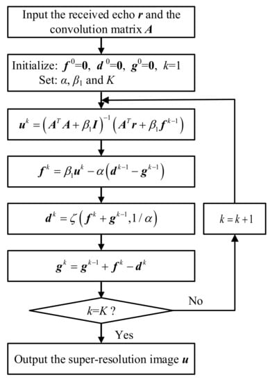
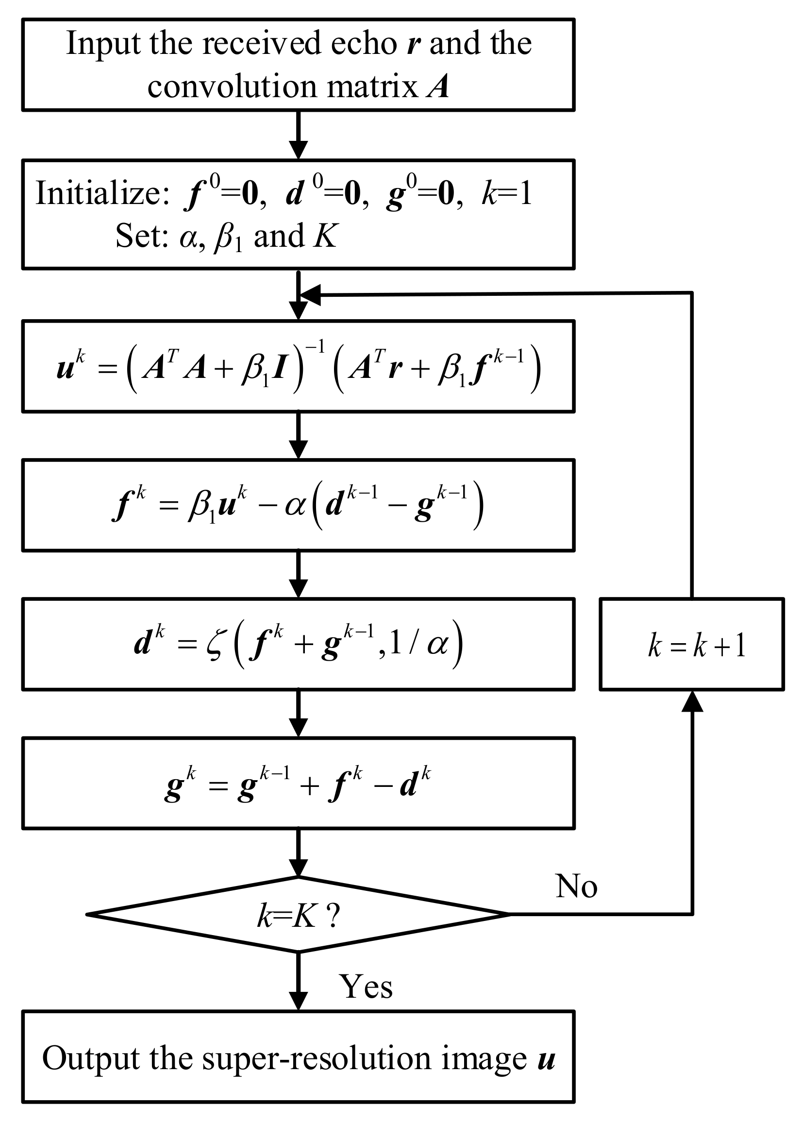
Therefore, for using the proposed SDBSM to achieve super-resolution imaging of scanning radar, the flowchart is show in Figure 1. The pseudocode code of SDBSM is shown in Appendix A.
Figure 1.
A flowchart of super resolution imaging using SDBSM.
3.2. Analysis of the Computational Complexity
The above deduction shows that SDBSM can be realized by four-step iteration, i.e., (14), (20), (22) and (18). After analysis, it can be seen that the main computational complexity comes from (14), which reaches the order of . As for (20), (22) and (18), only basic operations are included. Compared with (14), their computational complexity is negligible.
For (14), assume that the azimuth samples is N. The matrix is transposed to , and the computational complexity is . In the iterative process, and need to be calculated once, and the computational complexities are and , respectively, where can be obtained by fast Fourier transform with a computational complexity of [27]. Let ; then, the computational complexity of each iteration is . For the inversion of , the computational complexity is . Let ; the computational complexity of each iteration is and can be ignored. Then, multiply and with a computational complexity of . Therefore, the computational complexity of the proposed SDBSM is , where K is the number of iterations. It can be seen that the computational complexity of the proposed SDBSM is high. In the next study, we will analyze the reasons for the high computational complexity and accelerate the algorithm.
4. Experimental Verification of the Proposed SDBSM
In this section, we discuss the experiments conducted to demonstrate the performance of the proposed SDBSM. We consider two aspects of performance: the ability to distinguish adjacent targets and the ability to maintain the shape of the target. In addition, the experimental results are compared with some traditional super-resolution methods, including TSVDM [13], FTVM [27], IAA [40], MLE [32], MAPE [34] and SSM [37].
4.1. A Simulation of Strong-Point Targets
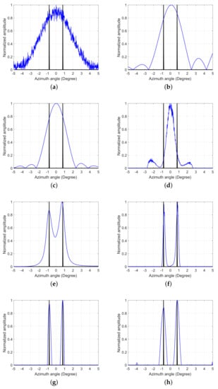
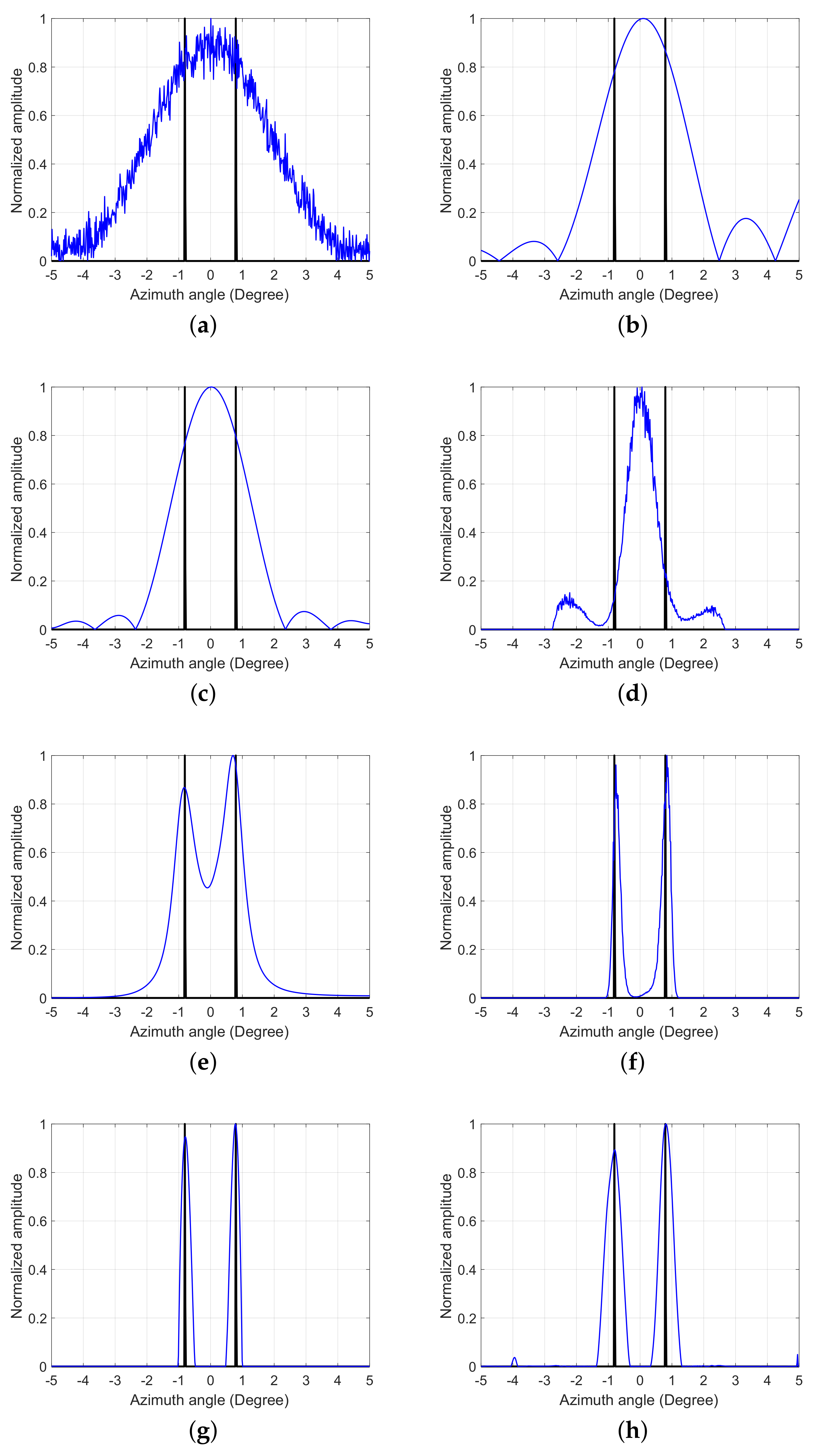
The first set of experiments were designed to verify the algorithm’s ability to distinguish adjacent targets. The original scene consisted of two adjacent strong-point targets at and with the same magnitude. The beam width of antenna pattern was . The scanning region was , the pulse repetition frequency (PRF) was 1000 Hz, the scanning speed was /s and the working distance was 2000 m. Based on the parameters, at 2000 m, the resolution of real-aperture imaging was approximately m, and the interval between adjacent targets was approximately m. The adjacent targets were not distinguished in real-aperture echo, in accordance with the Rayleigh resolution criterion.
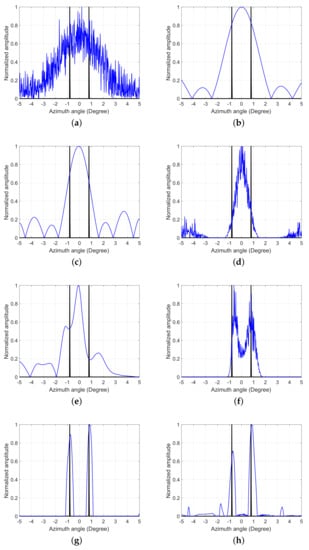
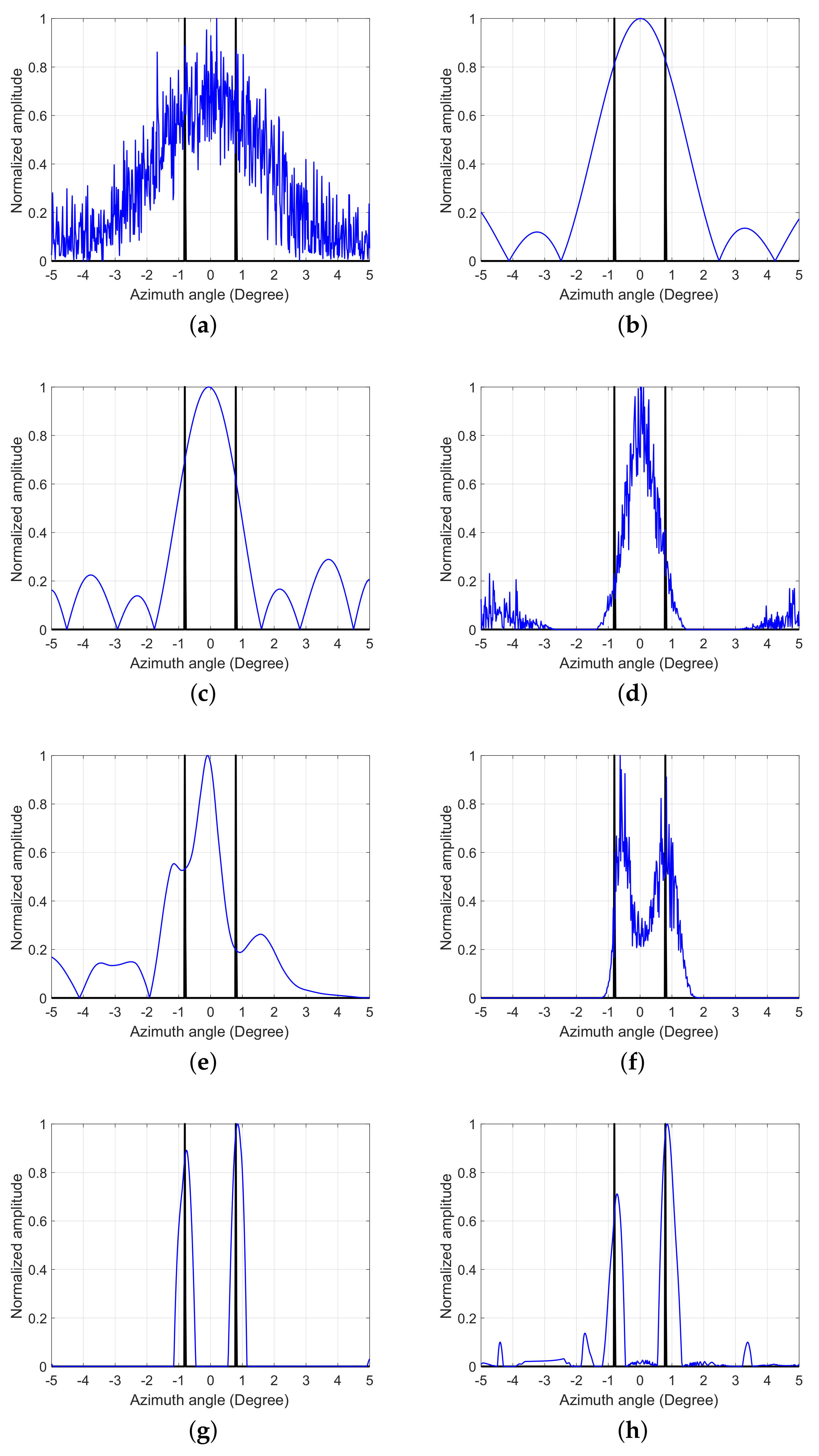
The simulation was first conducted under high-SNR conditions. We let and ; the simulation results are shown in Figure 2, where the black mark indicates the true distribution of the targets, and the blue mark indicates the processing results of different methods. Figure 2a shows the real-aperture echo with the SNR of 20 dB. It can be seen that the adjacent targets are not distinguishable. Figure 2b–h presents the processed results of different methods. From the results of TSVDM, FTVM and MLE shown in Figure 2b–d, it can be seen that TSVDM and FTVM only smoothed the noise and could not distinguish adjacent targets. Although MLE sharpened the echo, it could not distinguish adjacent targets. Figure 2e shows that IAA distinguished the adjacent targets and suppressed the noise, but the adjacent targets were not completely distinguished. It seems that there was still high adhesion between adjacent targets. Under the high SNR condition, MAPE, SSM and the proposed SDBSM could distinguish adjacent targets and suppress the noise, as Figure 2f–h show.
Figure 2.
Point targets simulation results with the SNR of . (a) Real-aperture echo. (b) Result processed by TSVDM. (c) Result processed by FTVM. (d) Result processed by MLE. (e) Result processed by IAA. (f) Result processed by MAPE. (g) Result processed by SSM. (h) Result processed by SDBSM.
Then, the above simulation was repeated under the condition of low SNR. In the simulation, SNR was set to 10 dB. The simulated results are shown in Figure 3. Under the condition of low SNR, the performances of all methods were degraded due to strong noise. The adjacent targets were not distinguishable by TSVDM, FTVM, MLE or IAA, as Figure 3b–e shows. Although MAPE seemed to be able to distinguish adjacent targets, the ability tp suppress noise deteriorated seriously, resulting in many burrs in the results, as shown in Figure 3f. Figure 3g shows that SSM still can distinguish the adjacent targets and suppress noise. For the proposed SDBSM, the result is shown in Figure 3h. Although adjacent targets are also identified, noise remains in non-target areas. It can be seen that the performance of SDBSM was slightly weaker than SSM under low-SNR conditions, but it was still superior to the other methods.
Figure 3.
Point targets simulation results with the SNR of . (a) Real-aperture echo. (b) Result processed by TSVDM. (c) Result processed by FTVM. (d) Result processed by MLE. (e) Result processed by IAA. (f) Result processed by MAPE. (g) Result processed by SSM. (h) Result processed by SDBSM.
At high SNR, IAA, MAPE, SSM and SDBSM could distinguish adjacent targets. At a low SNR, IAA could not distinguish adjacent targets. To quantitatively evaluate the performance of distinguishing adjacent targets, we introduced the beam sharpening ratio (BSR) for different methods. The BSR is defined as the ratio of the width of a single point before processing to its width after processing. The larger the BSR, the better the beam sharpening performance of the method, which is conducive to the distinguishing of adjacent targets.
The BSRs of different methods are shown in Table 1. It can be seen that the BSR of SDBSM was higher than that of IAA but lower than those of MAPE and SSM at high and low SNR. However, from the processing results shown in Figure 2 and Figure 3, it can be seen that MAPE amplified noise at a low SNR and the adjacent targets were not fully distinguished. SDBSM, however, was able to completely distinguish adjacent targets despite a decrease in noise suppression. As for SSM, its ability to distinguish adjacent targets (and suppress noise) was superior to that of SDBSM.
Table 1.
BSRs of different methods.
For this simulation, because the original scene contained two strong-point targets, it was very beneficial for SSM. Therefore, SSM achieved superior super-resolution performance to SDBSM. For targets with a typical shape, SSM may treat the target as a strong point and lose its shape. The next simulation sought to verify this conclusion.
4.2. Simulations of Area Targets
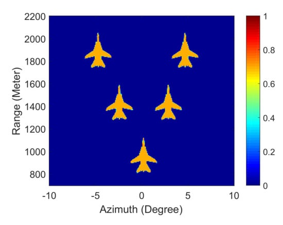
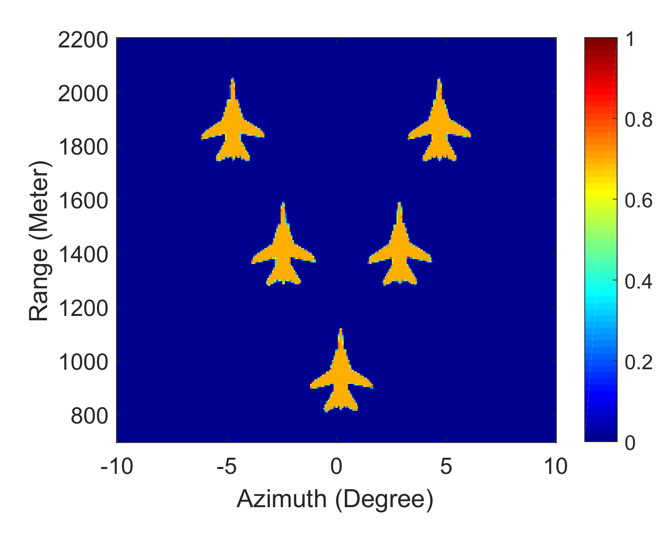
In order to verify the shape-preserving ability of SDBSM, an original scene was composed of five aircraft in a V-shape, as shown in Figure 4. It can be seen that there was an isolated aircraft at 900 m, and there were two adjacent aircraft at 1400 m and 1900 m. The beam width was , the scanning region was , the PRF was 1000 Hz and the scanning speed was /s.
Figure 4.
An original scene of the targets simulation.
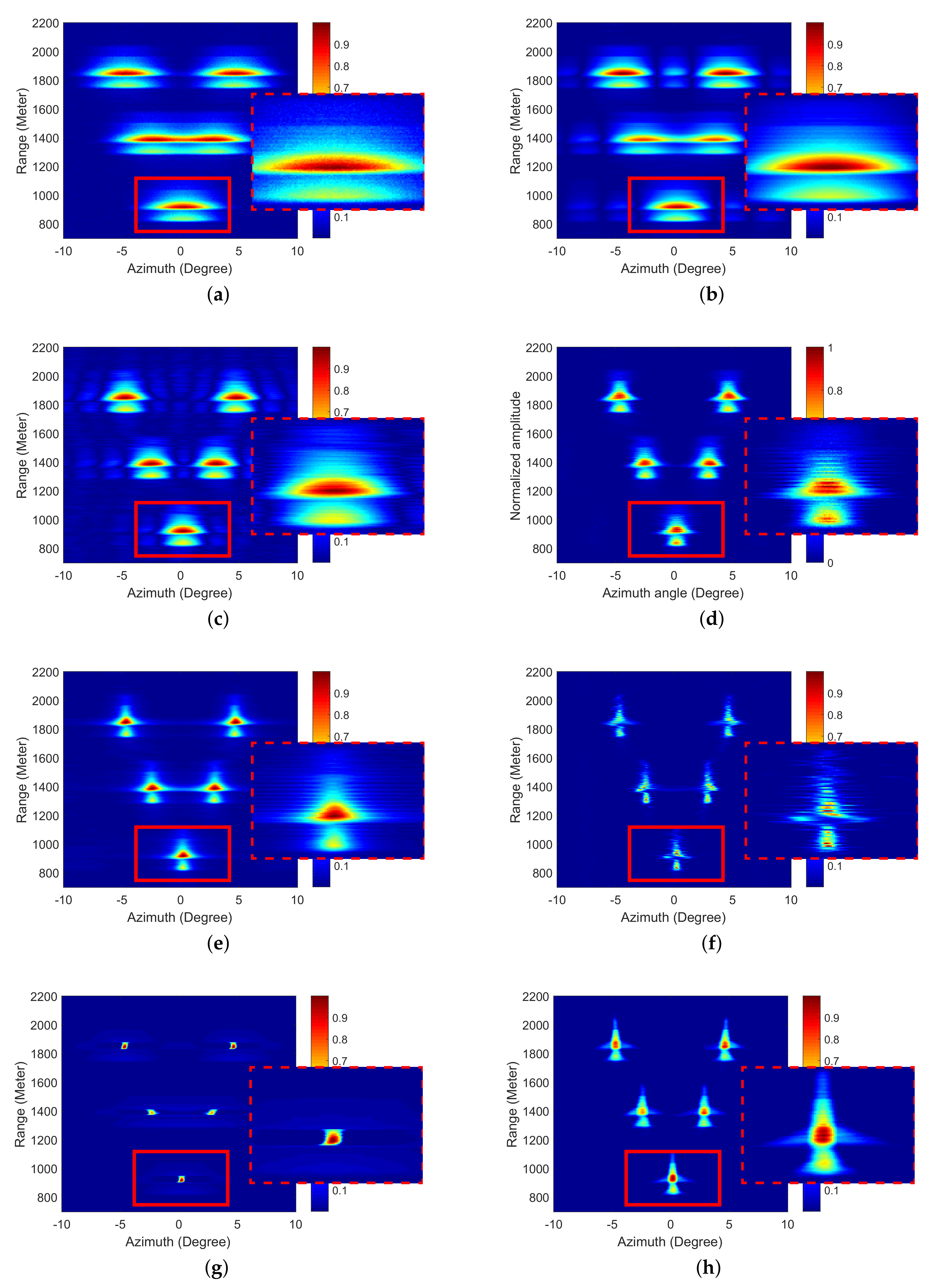
Similarly, the simulation was first conducted under high-SNR conditions, and the SNR of the real-aperture echo was 20 dB. The simulation results are shown in Figure 5. The red solid rectangle marks an isolated aircraft and was used to measure the performances of different methods in terms of preserving the shape of the target. The red dashed rectangle indicates partial enlarged drawings. Figure 5a presents the real-aperture echo. It can be seen that the adjacent aircraft at 1900 m was distinguished, but not the one at 1400 m, and the shape of the aircraft was blurred.
Figure 5.
Area targets simulation results with the SNR of 20 dB. (a) Real-aperture echo. (b) Result processed by TSVDM. (c) Result processed by FTVM. (d) Result processed by MLE. (e) Result processed by IAA. (f) Result processed by MAPE. (g) Result processed by SSM. (h) Result processed by SDBSM.
The results generated by the different methods are shown in Figure 5b–h. It shows that, for TSVDM, the improvement in the resolution was poor, and the adjacent aircraft at 1400 m was not distinguishable. FTVM could distinguish all the adjacent aircraft, but it was sensitive to noise. The noise was amplified to a certain degree. MLE, IAA and MAPE could distinguish the adjacent aircraft and suppress the noise, but the edges of the aircraft were fuzzy. SSM could also distinguish the adjacent aircraft, but because SSM regarded the target as a strong point, the shape of the target was completely lost. For the proposed SDBSM, we let and . It can be seen that it could not only distinguish the adjacent aircraft and suppress the noise, but it also maintained the shape of the planes. We can clearly see five planes in the processing results. The results of SDBSM are obviously clearer than those of other methods. Besides, from the partial enlarged drawings, we can obviously see that the edges of the aircraft are fuzzy in the results of TSVDM, FTVM, MLE, IAA and MAPE. The shape was completely lost by SSM. However, the edges of the aircraft are clearly preservated in the result of the proposed SDBSM.
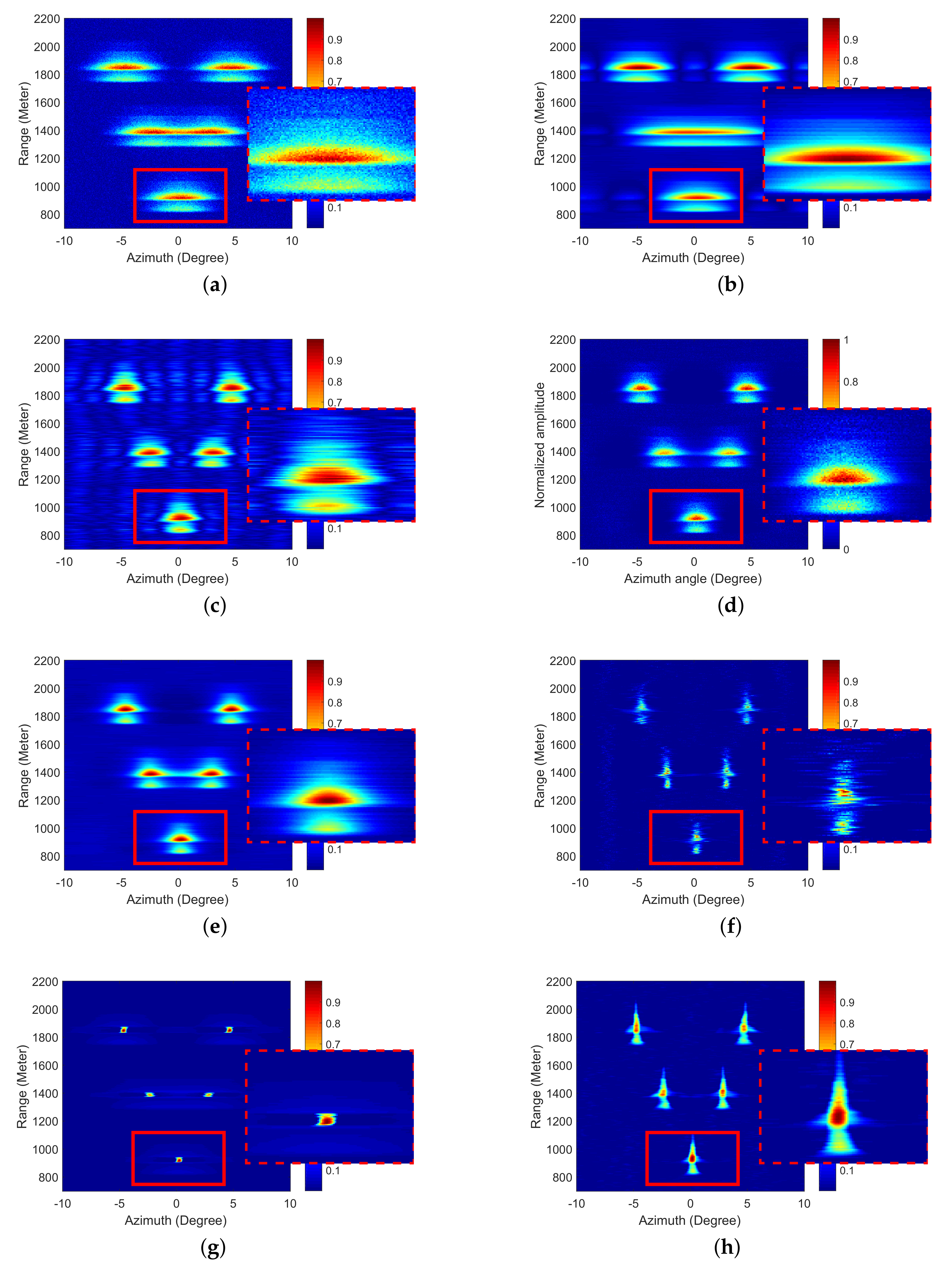
Next, the simulation results under low-SNR conditions are shown in Figure 6, wherein the SNR of the real-aperture echo was 10 dB. At the low SNR, the proposed SDBSM could also distinguish the adjacent aircraft, and the shape of the aircraft was preserved. The super-resolution performance proved superior to the other methods.
Figure 6.
Area targets simulation results with the SNR of 10 dB. (a) Real-aperture echo. (b) Result processed by TSVDM. (c) Result processed by FTVM. (d) Result processed by MLE. (e) Result processed by IAA. (f) Result processed by MAPE. (g) Result processed by SSM. (h) Result processed by SDBSM.
Visual observations show that the processing results of SDBSM were clearer than those of other methods. To quantitatively validate this conclusion, image entropy was introduced. According to the principle of minimum entropy, the entropy increases with an increase in the image blurring level [41]. The entropy can be calculated by the equation:
where E is the entropy, and is the proportion of pixels whose gray value is i after normalization.
By computation, the entropy of the results processed by different methods is shown in Table 2. It can be seen that the entropy of the results of the proposed SDBSM os lower than the entropies generated by other methods in both high and low-SNR conditions. According to the principle of minimum entropy, these findings show that the processing results of SDBSM are clearer than those of other methods, which is also in line with the visual observations.
Table 2.
Entropy of the results.
4.3. Real Data Verification
The performance of the proposed SDBSM has been demonstrated by simulations. Next, real airborne data were processed to verify the performance of SDBSM in practice. The real data were collected in the ancient town of Luodai, Chengdu. In this experiment, the radar system was suspended on a helicopter, and the antenna’s beam scanned the ground. The system parameters of the radar are shown in Table 3.
Table 3.
Parameters of the experiment.
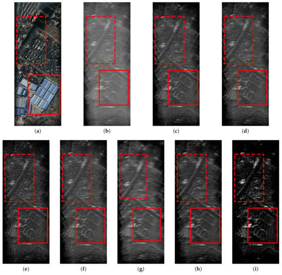
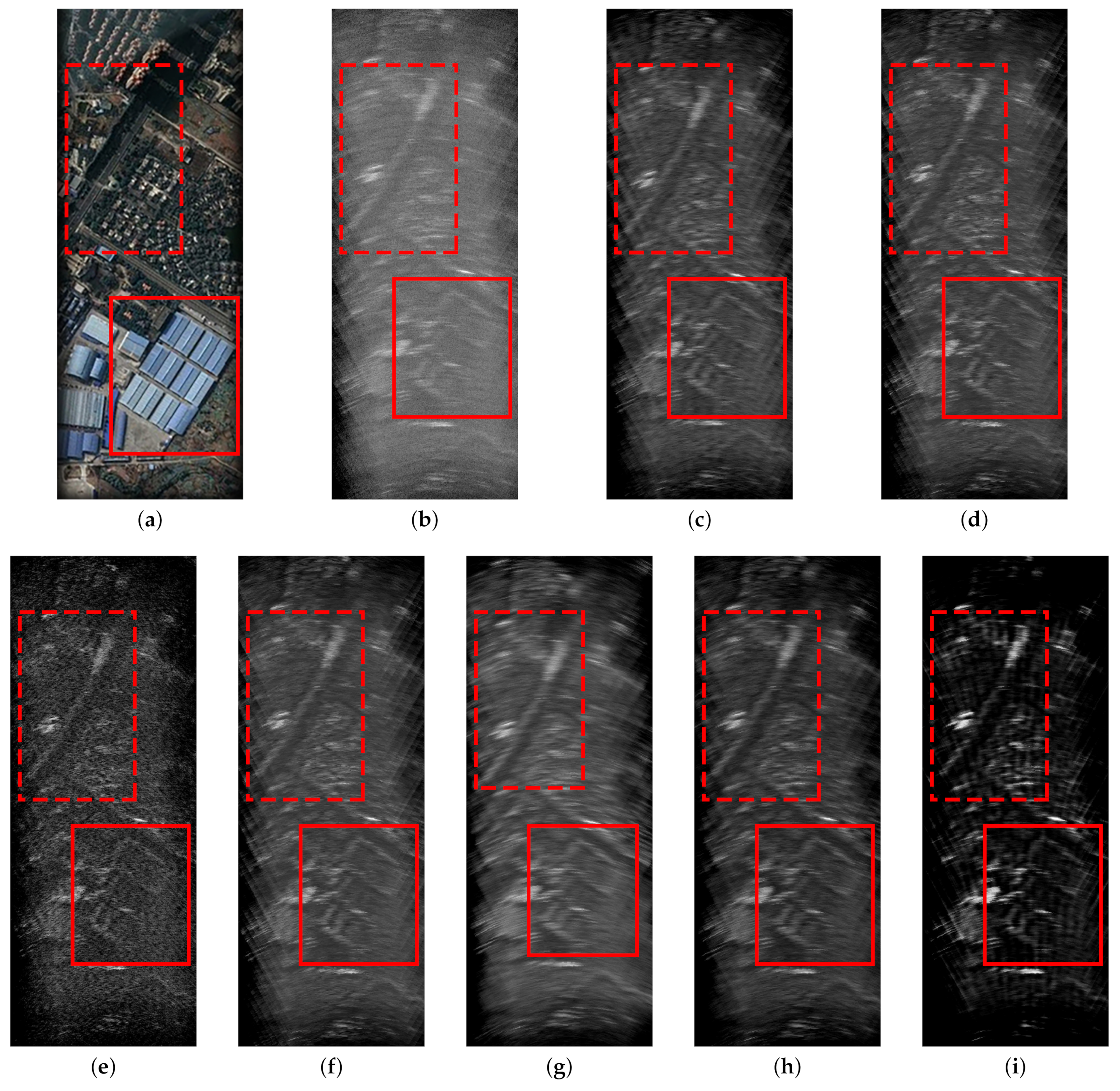
The results of the experiment are shown in Figure 7. Figure 7a shows the optical scene derived from Google Earth. The original scene contains distinct roads and houses, marked with red dashed rectangles and solid rectangles, respectively. The real-aperture echo with low resolution is shown in Figure 7b. The scene is blurry, and the houses and roads are not clear. Figure 7c,d presents the results processed by TSVDM and FTVM. It can be seen that the resolution improvement was greatly limited. Figure 7e shows the results processed by MLE. Although the resolution was improved, the edges of roads and houses were blurred. Figure 7f–h presents the results of IAA, MAPE and SSM. Although these methods were able to improve the resolution to a certain degree, the shapes of the roads and houses were not clear. Figure 7i shows the results of the proposed SDBSM. On the whole, the results of SDBSM were clearer than those of other methods, and the houses and roads were very distinct.
Figure 7.
Super-resolution results of real data. (a) Optical scenario. (b) Real-aperture echo. (c) Result processed by TSVDM. (d) Result processed by FTVM. (e) Result processed by MLE. (f) Result processed by IAA. (g) Result processed by MAPE. (h) Result processed by SSM. (i) Result processed by SDBSM.
Similarly to the area target simulation, we used image entropy to quantitatively evaluate the clarity of the processing results shown in Figure 7. The image entropy is shown in Table 4. We can see that the entropy of the proposed SDBSM was smaller than those of the other methods, demonstrating that the proposed SDBSM achieved a greater resolution improvement than the other methods.
Table 4.
Entropy and contrast of the real data results.
In addition, for the real data shown in Figure 7, we introduced image contrast to further measure their clarity [42]. From the perspective of image processing, the greater the contrast, the clearer the image. The contrast is defined as:
where C is the contrast, is the gray difference between adjacent pixels and is the pixel distribution probability of adjacent pixels with a gray difference of . The results are also shown in Table 4, which shows that the contrast of Figure 7i is higher than that of other images. It also shows that the processing results of the proposed SDBSM are clearer than those of the other methods.
5. Conclusions
In this paper, a SDBSM was proposed to improve the azimuth resolution for scanning radar imaging. The proposed SDBSM is an improvement over traditional SSM. Unlike traditional SSM, SDBSM introduces the norm for denoising and then achieves super-resolution imaging by cross-iteration of denoising and deconvolution.
From our experiments, we can draw the following conclusions: for the strong-point targets, the SSM method has a good super-resolution effect and can effectively distinguish the adjacent targets and suppress the noise. In contrast, the performance of SDBSM is slightly inferior. However, for a target with typical shape characteristics, although SSM can distinguish adjacent targets and suppress noise, the shape of the target is lost. SDBSM can not only distinguish the adjacent targets and suppress the noise, but also retain the shape information of the target better, which is helpful in the accurate identification of the specific shape of a target in practical applications.
Of course, as described in Section 3.2, SDBSM has high computational complexity. In practical applications, the real-time imaging ability needs to be improved. In the next step, we will accelerate the algorithm to improve its real-time imaging ability in practical applications.
Author Contributions
Conceptualization, Q.Z.; methodology, Q.Z., Y.Z. (Yin Zhang), Y.Z. (Yongchao Zhang); software, Q.Z.; validation, Q.Z. and Y.Z. (Yin Zhang); formal analysis, Q.Z.; investigation, Q.Z.; resources, Q.Z., Y.Z. (Yongchao Zhang), Y.H. and J.Y.; data curation, Q.Z.; writing—original draft preparation, Q.Z.; writing—review and editing, Q.Z.; visualization, Q.Z.; supervision, Y.Z. (Yin Zhang); project administration, Y.Z. (Yin Zhang); funding acquisition, Y.Z. (Yin Zhang), Y.Z. (Yongchao Zhang), Y.H. and J.Y. All authors have read and agreed to the published version of the manuscript.
Funding
This work was supported in part by the National Natural Science Foundation of China under Grant 61671117, 61901090 and 61901092.
Institutional Review Board Statement
Not applicable.
Informed Consent Statement
Not applicable.
Data Availability Statement
I exclude this statement because the study did not report any data.
Conflicts of Interest
The authors declare no conflict of interest.
Appendix A. Pseudocode of the Proposed SDBSM
function s = SDBSM(r,H,alpha,beta1,K) % r:echo; H: convolution matrix; K: iterations;
N = length(r);
I = eye(N);
s = zeros(N,1);
for i = 1:K
f = inv(H’*H+alpha*I)*(H’*r+alpha*((s)));
s = denoising(abs(f), beta1,alpha);
end
s = s./max(abs(s));
end
function u = denoising(y,miu,lambda)
N = length(y);
d = zeros(N,1); b = zeros(N,1);
u = miu*y + lambda*(d − b);
d = sign(u + b).*max(abs(u + b) − 1/lambda,0);
b = b + u − d;
end
References
- Zhang, Y.; Luo, J.; Li, J.; Mao, D.; Zhang, Y.; Huang, Y.; Yang, J. Fast inverse-scattering reconstruction for airborne high-squint radar imagery based on doppler centroid compensation. IEEE Trans. Geosci. Remote Sens. 2021. [Google Scholar] [CrossRef] [Scilit]
- North, K.W.; Oue, M.; Kollias, P.; Giangrande, S.E.; Collis, S.M.; Potvin, C.K. Vertical air motion retrievals in deep convective clouds using the ARM scanning radar network in oklahoma during MC3E. Atmos. Meas. Tech. 2017, 10, 2785–2806. [Google Scholar] [CrossRef] [Scilit]
- Albright, K.S. Environmental scanning: Radar for success. Inf. Manag. J. 2004, 38, 38–45. [Google Scholar]
- Zhang, Q.; Zhang, Y.; Huang, Y.; Zhang, Y.; Pei, J.; Yi, Q.; Li, W.; Yang, J. TV-sparse super-resolution method for radar forward-looking imaging. IEEE Trans. Geosci. Remote Sens. 2020, 58, 6534–6549. [Google Scholar] [CrossRef] [Scilit]
- Soldovieri, F.; Gennarelli, G.; Catapano, I.; Liao, D.; Dogaru, T.; Soldovieri, F.; Gennarelli, G.; Catapano, I.; Liao, D.; Dogaru, T. Forward-looking radar imaging: A comparison of two data processing strategies. IEEE J. Sel. Top. Appl. Earth Obs. Remote Sens. 2016, 10, 562–571. [Google Scholar] [CrossRef] [Scilit]
- Biondi, F. Recovery of partially corrupted SAR images by super-resolution based on spectrum extrapolation. IEEE Geosci. Remote Sens. Lett. 2016, 14, 139–143. [Google Scholar] [CrossRef] [Scilit]
- Rehacek, J.; Paúr, M.; Stoklasa, B.; Sánchez-Soto, L.L. Optimal measurements for resolution beyond the Rayleigh limit. Opt. Lett. 2017, 42, 231–234. [Google Scholar] [CrossRef] [Scilit]
- Davis, E.J.; Bridges, M.A. The Rayleigh limit of charge revisited: Light scattering from exploding droplets. J. Aerosol Sci. 1994, 25, 1179–1199. [Google Scholar] [CrossRef] [Scilit]
- Dropkin, H.; Ly, C. Superresolution for scanning antenna. In Proceedings of the 1997 IEEE National Radar Conference, Syracuse, NY, USA, 13–15 May 1997; pp. 306–308. [Google Scholar]
- Li, Y.; Liu, J.; Jiang, X.; Huang, X. Angular superresol for signal model in coherent scanning radars. IEEE Trans. Aerosp. Electron. Syst. 2019, 55, 3103–3116. [Google Scholar] [CrossRef]
- Sadjadi, F. Radar beam sharpening using an optimum FIR filter. Circuits Syst. Signal Process. 2000, 19, 121–129. [Google Scholar] [CrossRef] [Scilit]
- Hansen, P.C. Truncated singular value decomposition solutions to discrete ill-posed problems with ill-determined numerical rank. Siam J. Sci. Stat. Comput. 1990, 11, 503–518. [Google Scholar] [CrossRef] [Scilit]
- Gao, P.; Rong, J.; Pu, H.; Liu, T.; Zhang, W.; Zhang, X.; Lu, H. Sparse view cone beam x-ray luminescence tomography based on truncated singular value decomposition. Opt. Express 2018, 26, 23233–23250. [Google Scholar] [CrossRef] [Scilit]
- Doğu, S.; Akıncı, M.N.; Çayören, M.; Akduman, I. Truncated singular value decomposition for through-the-wall microwave imaging application. IET Microw. Antennas Propag. 2019, 14, 260–267. [Google Scholar] [CrossRef] [Scilit]
- Li, J.; Stoica, P.; Wang, Z. On robust Capon beamforming and diagonal loading. IEEE Trans. Signal Process. 2003, 51, 1702–1715. [Google Scholar]
- Zhang, H.; López-Dekker, P. Persistent scatterer densification through the application of capon-and apes-based sar reprocessing algorithms. IEEE Trans. Geosci. Remote Sens. 2019, 57, 7521–7533. [Google Scholar] [CrossRef]
- Cheney, M. The linear sampling method and the MUSIC algorithm. Inverse Probl. 2001, 17, 591. [Google Scholar] [CrossRef] [Scilit]
- Zhang, D.; Zhang, Y.; Zheng, G.; Feng, C.; Tang, J. Improved DOA estimation algorithm for co-prime linear arrays using root-MUSIC algorithm. Electron. Lett. 2017, 53, 1277–1279. [Google Scholar] [CrossRef] [Scilit]
- Guili, Z.; Youming, L.I.; Mingchen, Y.U.; Wang, X. Impulsive noise mitigation based on iteration adaptive approach in underwater acoustic communication. Telecommun. Sci. 2017, 33, 66. [Google Scholar]
- Glentis, G.O.; Jakobsson, A. Efficient implementation of iterative adaptive approach spectral estimation techniques. IEEE Trans. Signal Process. 2011, 59, 4154–4167. [Google Scholar] [CrossRef] [Scilit]
- Zhang, Y.; Mao, D.; Zhang, Q.; Zhang, Y.; Huang, Y.; Yang, J. Airborne forward-looking radar super-resolution imaging using iterative adaptive approach. IEEE J. Sel. Top. Appl. Earth Obs. Remote Sens. 2019, 12, 2044–2054. [Google Scholar] [CrossRef] [Scilit]
- Zhang, Y.; Zhang, Y.; Li, W.; Huang, Y.; Yang, J. Super-Resolution Surface Mapping for Scanning Radar: Inverse Filtering Based on the Fast Iterative Adaptive Approach. IEEE Trans. Geosci. Remote Sens. 2018, 56, 127–144. [Google Scholar] [CrossRef] [Scilit]
- Rudin, L.I.; Osher, S.; Fatemi, E. Nonlinear total variation based noise removal algorithms. Phys. D Nonlinear Phenom. 1992, 60, 259–268. [Google Scholar] [CrossRef] [Scilit]
- Yang, J.H.; Zhao, X.L.; Ma, T.H. Remote sensing images destriping using unidirectional hybrid total variation and nonconvex low-rank regularization. J. Comput. Appl. Math. 2020, 363, 124–144. [Google Scholar] [CrossRef] [Scilit]
- Wang, Y.; Peng, J.; Zhao, Q.; Leung, Y.; Zhao, X.-L.; Meng, D. Hyperspectral image restoration via total variation regularized low-rank tensor decomposition. IEEE J. Sel. Top. Appl. Earth Obs. Remote Sens. 2017, 11, 1227–1243. [Google Scholar] [CrossRef] [Scilit]
- Thanh, D.N.H.; Thanh, L.T.; Hien, N.N.; Prasath, S. Adaptive total variation L1 regularization for salt and pepper image denoising. Optik 2020, 208, 163677. [Google Scholar] [CrossRef] [Scilit]
- Zhang, Q.; Zhang, Y.; Zhang, Y.; Huang, Y.; Yang, J. Airborne radar super-resolution imaging based on fast total variation method. Remote Sens. 2021, 13, 549. [Google Scholar] [CrossRef] [Scilit]
- Peng, J.; Li, L.; Tang, Y.Y. Maximum likelihood estimation-based joint sparse representation for the classification of hyperspectral remote sensing images. IEEE Trans. Neural Netw. Learn. Syst. 2018, 30, 1790–1802. [Google Scholar] [CrossRef] [Scilit]
- Li, K.; Peng, S.; Zhang, T.; Malik, J. Multimodal image synthesis with conditional implicit maximum likelihood estimation. Int. J. Comput. Vis. 2020, 128, 2607–2628. [Google Scholar] [CrossRef] [Scilit]
- Shao, J.; Liao, W.-C.; Liang, R.; Barnard, K. Resolution enhancement for fiber bundle imaging using maximum a posteriori estimation. Opt. Lett. 2018, 43, 1906–1909. [Google Scholar] [CrossRef] [Scilit]
- Anandhi, D.; Valli, S. An algorithm for multi-sensor image fusion using maximum a posteriori and nonsubsampled contourlet transform. Comput. Electr. Eng. 2018, 65, 139–152. [Google Scholar] [CrossRef] [Scilit]
- Tan, K.; Li, W.; Zhang, Q.; Huang, Y.; Wu, J.; Yang, J. Penalized maximum likelihood angular super-resolution method for scanning radar forward-looking imaging. Sensors 2018, 18, 912. [Google Scholar] [CrossRef] [Scilit]
- Hunziker, J.; Laloy, E.; Linde, N. Bayesian full-waveform tomography with application to crosshole ground penetrating radar data. Geophys. J. Int. 2019, 218, 913–931. [Google Scholar] [CrossRef] [Scilit]
- Wu, Q.; Lai, Z.; Amin, M.G. Through-the-wall radar imaging based on Bayesian compressive sensing exploiting multipath and target structure. IEEE Trans. Comput. Imaging 2021, 7, 422–435. [Google Scholar] [CrossRef] [Scilit]
- Shao, Z.; Wang, L.; Wang, Z.; Deng, J. Remote sensing image super-resolution using sparse representation and coupled sparse autoencoder. IEEE J. Sel. Top. Appl. Earth Obs. Remote. Sens. 2019, 12, 2663–2674. [Google Scholar] [CrossRef] [Scilit]
- Poon, C.; Peyré, G. Multidimensional sparse super-resolution. SIAM J. Math. Anal. 2019, 51, 1–44. [Google Scholar] [CrossRef] [Scilit]
- Zhang, Q.; Zhang, Y.; Huang, Y.; Zhang, Y. Azimuth superresolution of forward-looking radar imaging which relies on linearized Bregman. IEEE J. Sel. Top. Appl. Earth Obs. Remote Sens. 2019, 12, 2032–2043. [Google Scholar] [CrossRef] [Scilit]
- Zhang, Y.; Jakobsson, A.; Zhang, Y.; Huang, Y.; Yang, J. Wideband sparse reconstruction for scanning radar. IEEE Trans. Geosci. Remote Sens. 2018, 56, 6055–6068. [Google Scholar] [CrossRef] [Scilit]
- Goldstein, T.; Osher, S. The split Bregman method for L1-regularized problems. SIAM J. Imaging Sci. 2009, 2, 323–343. [Google Scholar] [CrossRef] [Scilit]
- Raju, C.; Reddy, T.S. MST radar signal processing using iterative adaptive approach. Geosci. Lett. 2018, 5, 20. [Google Scholar] [CrossRef] [Scilit]
- Ke, L.; Marcellin, M.W. Near-lossless image compression: Minimum-entropy, constrained-error dpcm. Image Process. IEEE Trans. 1998, 7, 225–228. [Google Scholar]
- Cai, J.; Gu, S.; Zhang, L. Learning a deep single image contrast enhancer from multi-exposure images. IEEE Trans. Image Process. 2018, 27, 2049–2062. [Google Scholar] [CrossRef] [Scilit] [PubMed]

Publisher’s Note: MDPI stays neutral with regard to jurisdictional claims in published maps and institutional affiliations. |
© 2021 by the authors. Licensee MDPI, Basel, Switzerland. This article is an open access article distributed under the terms and conditions of the Creative Commons Attribution (CC BY) license (https://creativecommons.org/licenses/by/4.0/).