Article

Fine-Resolution Mapping of Pan-Arctic Lake Ice-Off Phenology Based on Dense Sentinel-2 Time Series Data

1
School of Geospatial Engineering and Science, Sun Yat-Sen University, Guangzhou 510275, China
2
Southern Marine Science and Engineering Guangdong Laboratory (Zhuhai), Zhuhai 519000, China
*
Author to whom correspondence should be addressed.
Remote Sens. 2021, 13(14), 2742; https://doi.org/10.3390/rs13142742
Submission received: 13 May 2021 / Revised: 30 June 2021 / Accepted: 7 July 2021 / Published: 13 July 2021
(This article belongs to the Special Issue Temporal Resolution, a Key Factor in Environmental Risk Assessment)

Abstract

:
The timing of lake ice-off regulates biotic and abiotic processes in Arctic ecosystems. Due to the coarse spatial and temporal resolution of available satellite data, previous studies mainly focused on lake-scale investigations of melting/freezing, hindering the detection of subtle patterns within heterogeneous landscapes. To fill this knowledge gap, we developed a new approach for fine-resolution mapping of Pan-Arctic lake ice-off phenology. Using the Scene Classification Layer data derived from dense Sentinel-2 time series images, we estimated the pixel-by-pixel ice break-up end date information by seeking the transition time point when the pixel is completely free of ice. Applying this approach on the Google Earth Engine platform, we mapped the spatial distribution of the break-up end date for 45,532 lakes across the entire Arctic (except for Greenland) for the year 2019. The evaluation results suggested that our estimations matched well with both in situ measurements and an existing lake ice phenology product. Based on the generated map, we estimated that the average break-up end time of Pan-Arctic lakes is 172 ± 13.4 (measured in day of year) for the year 2019. The mapped lake ice-off phenology exhibits a latitudinal gradient, with a linear slope of 1.02 days per degree from 55°N onward. We also demonstrated the importance of lake and landscape characteristics in affecting spring lake ice melting. The proposed approach offers new possibilities for monitoring the seasonal Arctic lake ice freeze–thaw cycle, benefiting the ongoing efforts of combating and adapting to climate change.

1. Introduction

Lakes, through their seasonal ice cover extent and duration, are a major landscape in the Arctic [1,2,3,4,5]. Governed by both geographical and morphological settings, the spring lake ice phenology (i.e., timing of ice-off) is a primary driver of Arctic hydrological processes [6], and has been identified as a sensitive metric to measure climate change [7,8,9]. Regional coherence or synchrony of lake break-up timing also regulates greenhouse gas emissions from fresh water into the atmosphere [9,10,11,12], affecting the land surface energy balance [13], which in turn generates feedbacks into the climate system. Given their wide-ranging importance, accurately estimating the spatial distribution of lake ice-off phenology is essential to understand Arctic ecosystem functions and project their responses to global environmental dynamics under various climate change scenarios [14,15].
Before the advent of remote sensing, lake ice-off phenology data could only be collected through in-field observations, which are nevertheless laborious and spatially sparse [16]. Satellite remote sensing has revolutionized our ability to monitor fresh water freeze–thaw cycling processes, especially at the continental to global scales [17]. Using high temporal frequency satellite image time series, many attempts have been made to extract lake ice-off timing information [18]. The microwave brightness temperature, with long available archives and the all-weather imaging capability, is perhaps the most widely used data source for lake ice phenology parameter identification [15,19,20,21]. However, most of the passive microwave sensors have coarse spatial resolutions (typically ranging from 6.25 km to 25 km), hence limiting their effectiveness within heterogeneous landscapes [15]. Therefore, other remote sensing data types with higher spatial resolutions, including synthetic aperture radar (SAR) [7,22], optical imagery [8,9,23,24], and UAV [25], have also been used for mapping lake ice-off phenology.
Despite previous efforts at estimating fresh water freeze–thaw cycling in many regions of the world, the extent and distribution of lake ice-off phenology have not yet been quantified across the entire Arctic, which vary with respect to ground thermal regime, topography, surface geology, and land cover [3]. Moreover, most of the current studies have been conducted by treating a lake as the smallest unit of interest, concealing the internal variability of lake ice-off timing distribution [26]. Technical challenges exist in almost every aspect of lake ice phenology mapping, including data acquisition, lake extent extraction, time series modeling, and ice melting/freezing identification. These challenges are even more critical for small lakes (typically less than 1000 ha), which account for approximately 99% of the total Arctic lake population [1], and which are more sensitive to climate change and land disturbance events [9,27].
This study aims to develop a spatially continuous map that first estimates Pan-Arctic lake ice-off phenology at a fine spatial resolution (i.e., 20 m). To achieve this goal, we design a new approach that identifies the per-pixel ice break-up date during the spring melting season based on dense time series stacks of Sentinel-2 data. We implement the algorithm on the Google Earth Engine (GEE) platform and apply it to lakes across the Pan-Arctic region (except for Greenland). To evaluate the mapping performance, we compare our results with those derived from daily freeze–thaw satellite products as well as in situ data for validation. In the remainder of this paper, we introduce the materials and methods (Section 2), report on the validation and mapping results of the Arctic lake ice-off phenology (Section 3), present discussions (Section 4), and draw some conclusions from the study (Section 5).

2. Materials and Methods

2.1. Study Area Boundaries and Lake Selection

The study area covers the entire Arctic, which is defined as the northernmost part of the Earth featured by tundra vegetation, an arctic climate, and arctic flora, with the tree line and the coastline joint-shaping its extent borders (Figure 1a) [27,28,29]. The lake selection in this study was based on HydroLAKES [30], which provides the shoreline polygons of global lakes with a surface area of no less than 10 ha. We filtered the HydroLAKES dataset by the extent of the study area, and excluded lakes that have a surface area less than 1 km2 to avoid noise introduced by mixing pixels at the shore line [8]. We also masked out supraglacial lakes in Greenland because of their inter-annual fluctuations in extent and distribution [31]. After the abovementioned selection procedure, there remained 47,230 lakes, ranging from 1 km2 to 4909 km2, with their spatial concentration displayed in Figure 1b.

2.2. Datasets

Our primary data source used was Sentinel-2 A/B satellite imagery, accessed from the European Space Agency (https://sentinel.esa.int/web/sentinel/user-guides/sentinel-2-msi, (accessed on 23 November 2020)) via the GEE platform [32]. Among the various Sentinel-2 products, we selected the category of Level 2A because it meets the formal quality of orthorectified Bottom-of-Atmosphere (BOA) reflectance, and thus multi-temporal images can be directly used to construct time series for further analysis [33]. Within the Sentinel-2 Level 2A data, we used mainly the Scene Classification Layer (termed SCL hereafter) band for lake ice-off phenology mapping at a 20 m resolution. For each Sentinel-2 image, the SCL band is a pixel classification map derived from four technical steps: cloud/snow detection, cirrus detection, cloud shadow detection, and classification map generation. A specific land cover scheme is designed for classifying each pixel into 11 different categories, including cloud, cloud shadows, vegetation, soils/deserts, water, snow/ice, etc. Readers can refer to the Sentinel-2 Level-2A Algorithm Overview (https://sentinels.copernicus.eu/web/sentinel/technical-guides/sentinel-2-msi/level-2a/algorithm, (accessed on 28 November 2020)) for more technical details of SCL generation. We processed all Sentinel-2 Level 2A data with less than 85% cloud obscuration acquired between 1 February and 1 September 2019, a collection of 1621 images with their average revisit interval pattern displayed in Figure 1c. In addition to satellite imagery, we also obtained ERA5 air temperature (ERA5 Ta hereafter), which is a reanalysis product that combines modeled data with observations into a globally gridded dataset, developed by the European Centre for Medium-Range Weather Forecasts (ECMWF). Compared with its predecessors, ERA5 Ta benefits from an enhanced spatial resolution and is becoming increasingly popular in lake/river ice applications [15,17]. Similar to the Sentinel-2 data collection, we accessed ERA5 Ta from the GEE’s public data archive, and utilized the daily average air temperature at 2 m height for better identification of the ice-melting timing information.

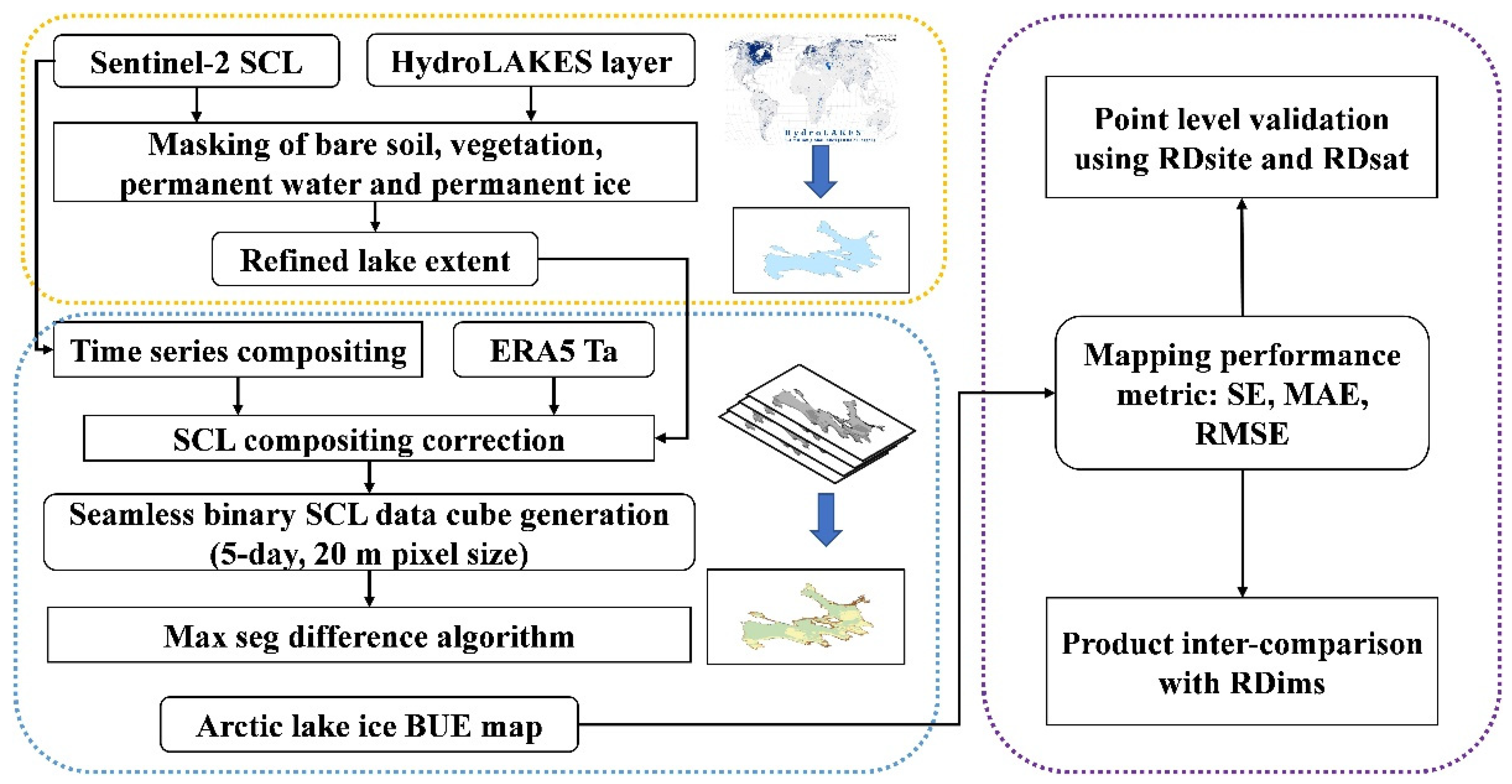
2.3. Lake Ice-Off Phenology Mapping Algorithm

Many ice phenology variables have been used for characterizing the spring melting process at the level of a pixel or lake. Here, we mainly focus on break-up end (BUE), which is defined as the day of the year (DOY) when the pixel becomes totally ice free [20,24]. Figure 2 displays the proposed approach that aims to utilize pixel-level SCL time series information for BUE mapping on the GEE platform. Particularly, the framework includes three sequentially integrated parts. In the first part, we refined the lake extent derived from HydroLAKES. This procedure was implemented by referring to Sentinel-2 SCL class information (Section 2.3.1). In the second part, we again used time series of Sentinel-2 SCL and ERA5 Ta to generate a seamless, binary phenophase time series at the 20 m resolution and 5-day interval. Then, such a dataset was utilized as the input of the “max-seg-difference” algorithm, which identifies the per-pixel BUE by seeking the transition time point when the pixel is completely free of ice (Section 2.3.2). Finally, we performed an accuracy assessment (Section 2.3.3) and analyzed the spatial pattern of our estimated lake ice-off phenology result across the entire Arctic (Section 2.3.4).

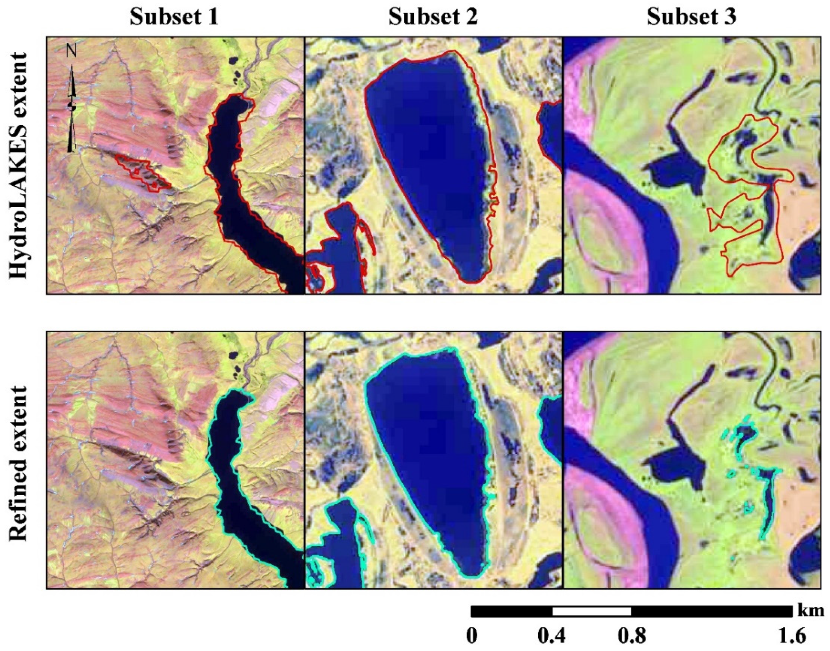
2.3.1. Lake Extent Refinement

Despite overall high accuracy, the HydroLAKES shoreline layer still bears errors for lake ice-off phenology mapping. Some waterbodies are frozen or clear of ice all year round, neither of which should be included in our analysis. Moreover, several Arctic lakes may have changed in their extents [34] or seasonal fluctuation patterns [35] since the release of HydroLAKES. Therefore, a lake extent refinement is required in this study. We rasterized the original HydroLAKES shoreline layer into a binary image consisting of two types: lake and non-lake. Then, a frequency threshold-based method [36,37] was applied only to the lake pixels for selecting waterbodies with seasonal ice duration based on Sentinel-2 SCL data. In particular, for pixel i , only by satisfying the following criterion can it be identified as valid and used for lake ice BUE mapping.
P i = { 1 ,   F b a r e 10 %   a n d   F v e g 10 %   a n d   F i c e 10 %   a n d   F w a t e r 10 % 0 ,   o t h e r w i s e
where P i is the final lake extent refinement result, with “1” denoting valid and “0” invalid. F b a r e , F v e g , F i c e , and F w a t e r are percentages of the SCL time series classified as bare soil, vegetation, water, and ice, respectively, within the study period (from 1 February 2019 to 1 September 2019). The threshold of 10% was adopted due to the overall classification uncertainty of the SCL data [38]. To evaluate the refined lake extent result, 800 stratified random sample points were selected, with one half collected within the refined lake extent while the other half from the masked regions. After removing points that were unable to be identified, there remained 324 and 325 sample points, respectively. Three metrics, including commission error, omission error, and F1 score, were selected for refinement assessment [39]. Here, commission and omission represent the percentage of valid lake samples that were falsely masked, and the percentage of invalid lake samples that were not detected by the refinement procedure, respectively. The F1 score quantifies the level of balance between precision (commission) and recall (omission).

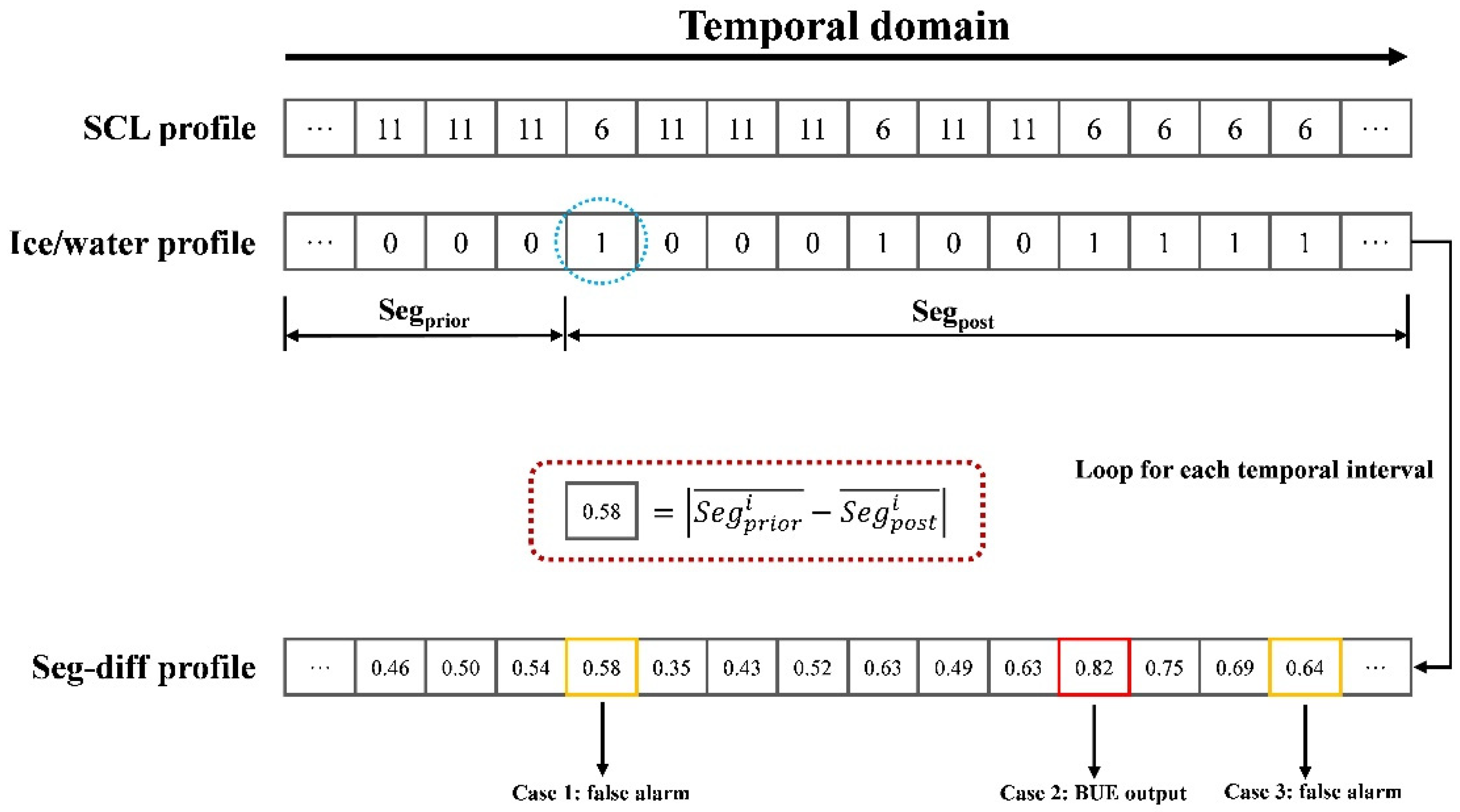
2.3.2. BUE Identification

  • Creation of phenophase time series
At the pixel level, this study used Sentinel-2 SCL data to create a binary (ice/water) phenophase time series. Within the refined lake extent, we first masked poor quality or irrelevant observations, leaving only observations classified as water or ice by the SCL (labeled as 6 and 11, respectively). Second, an equitemporal phenophase composite was obtained by deriving the mode value of all valid observations during each temporal interval, which was set to 5 days as a balance of multiple factors, including the sensor revisit cycle, swath (the area imaged on Earth surface) overlap, and the temporal uncertainty control of the final BUE map. It should be noted that an extreme case may exist; that is, in a 5-day interval, there might be no valid data from any Sentinel-2 observations. In this case, a filling value was determined according to temporally adjacent (within 15 days) valid observations.
  • Outlier removal
Several outliers remain in the created phenophase data cube because of the misclassification errors of the SCL. These errors on the temporal dimension could undermine or even lead to the failure of the BUE identification. In this study, we used ERA5 Ta data for outlier removal because the lake ice melting is highly correlated to the warming process of air temperature [9,25,40]. Due to the spatial resolution mismatch, the bicubic interpolation algorithm [41] was used for resizing the original ERA5 Ta data to 20 m, and the 28-day average air temperature ( T a 28 ) was adopted as the metric to correct unreasonable ice or water presence [9]. Two threshold values, −5 °C and 5 °C, were selected, corresponding to the upper and lower boundaries of T a 28 when the outlier removal takes effect. Specifically, two situations are involved. In the first situation, we assume no ice should melt if T a 28 is equal or lower than −5 °C. By contrast, in the second situation, we assume no ice should exist when T a 28 is equal or higher than 5 °C. Such a threshold filter approach has been widely applied in previous studies [9,42], and proven effective for reducing the spurious detection results of ice melting.
  • The “max-seg-difference” algorithm
Traditionally, the lake ice BUE is identified from satellite sensors by detecting a sharp change in surface reflectance or brightness temperature trajectory during the spring melting period [8,43]. This method is straightforward, but its usefulness could be affected by a number of factors, including sun illumination [8], ice thickness [25], and microwave dielectric properties [22]. As a consequence, additional intervention from the user is usually needed, hampering the application of BUE mapping over large areas. To deal with this issue, here we proposed a new BUE identification algorithm, aiming to be more self-adaptive at the per-pixel level through segmentation of the phenophase time series. Figure 3 graphically displays how the BUE date is determined for one pixel. First, we used the SCL trajectory to create a new Boolean time series profile, indicating the phenophase (water as 1, ice as 0) at each temporal interval. Then, for a given temporal interval D O Y i (highlighted with the blue circle), the entire phenophase profile can be divided into two parts: S e g p r i o r i and S e g p o s t i , with D O Y i as the boundary point. Since BUE represents the ending of ice cover and the beginning of open water, our core target here is to find a temporal interval D O Y m a x when the difference between S e g p r i o r i (ice dominated) and S e g p o s t i (water dominated) can be maximized. The objective function is thus written as
arg m a x   | S e g ¯ p r i o r i S e g ¯ p o s t i | ,   i [ 1 ,   N ]
where S e g ¯ p r i o r i and S e g ¯ p o s t i are the average values of S e g p r i o r i and S e g p o s t i , respectively, and N is the length of the temporal domain (the total number of temporal intervals). In practice, we created a loop for each temporal interval and generated a “seg-diff” profile, through which BUE can be identified according to the maximum principle. A primary advantage of the “max-seg-difference” algorithm is that it can make full use of the time series information so that the impacts of “false” alarms (e.g., Case 1 and Case 3 in Figure 3) would be greatly reduced or even eliminated. We implemented the “max-seg-difference” algorithm within the refined lake extent using GEE, and the final Pan-Arctic BUE map were produced and exported at a 20 m spatial resolution.

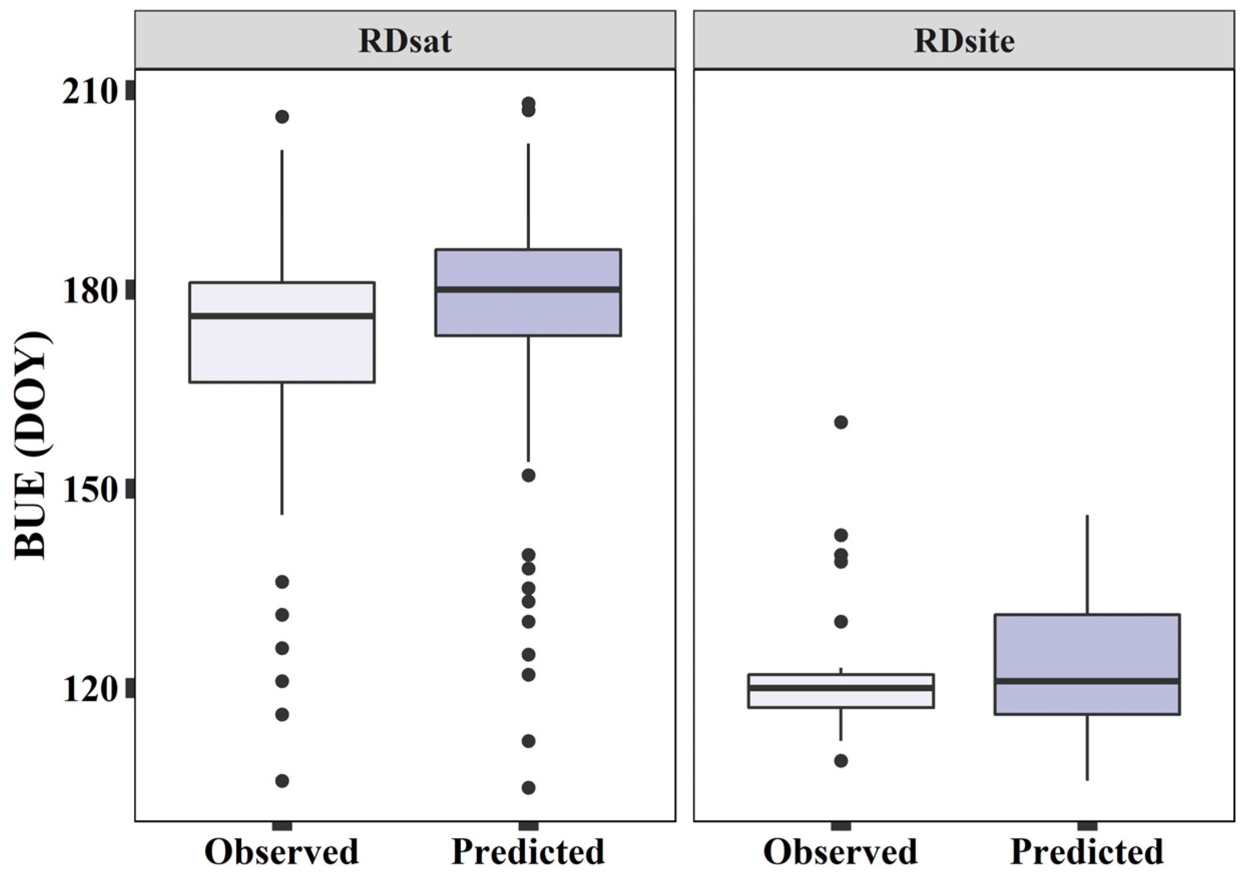
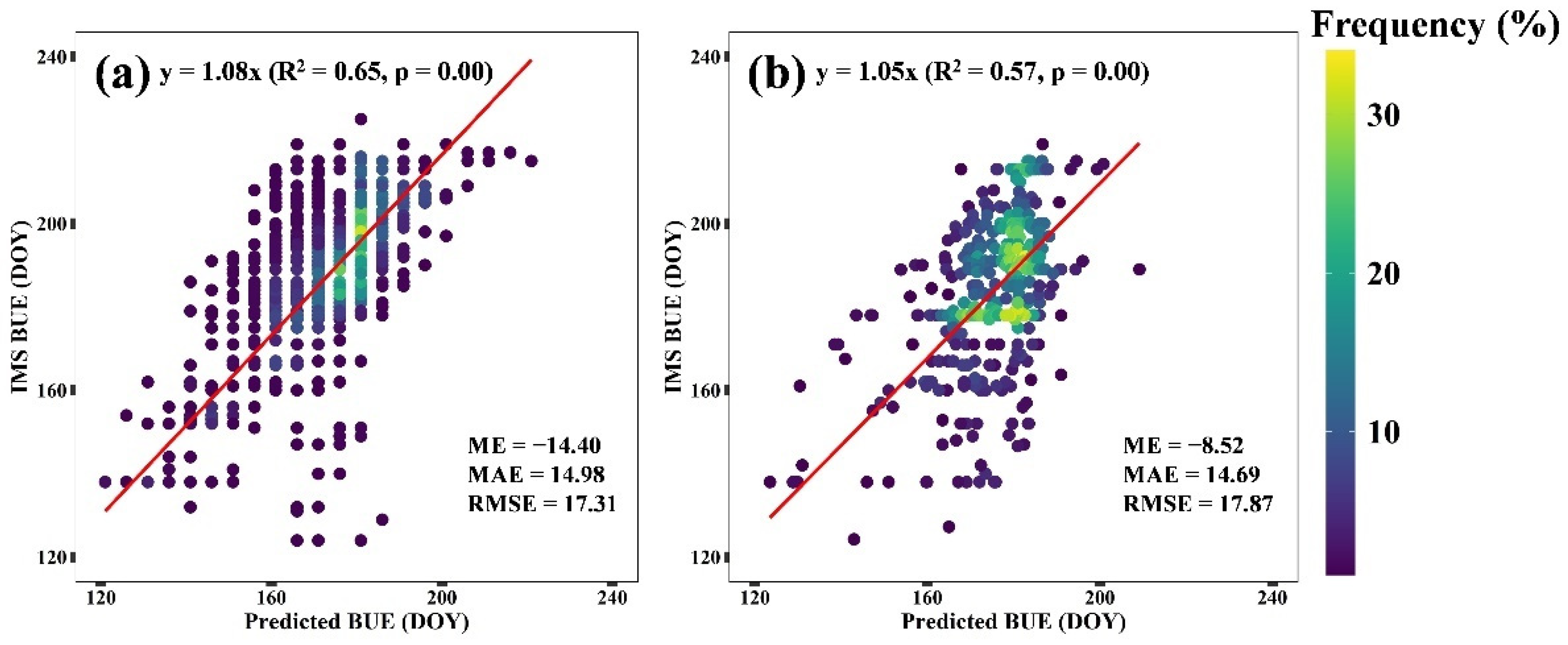
2.3.3. Evaluation of Lake Ice-Off Phenology Mapping

The performance evaluation of the Pan-Arctic lake ice BUE map was conducted in two ways. In the first evaluation method, we randomly created 400 sample points within the refined lake extent, and their BUE dates for the year 2019 were visually identified based on multi-temporal satellite images, including Sentinel-1, Sentinel-2, Landsat-8, and Planet, for the purpose of interpretation bias minimization. We kept only well-interpreted points with a high level of confidence, which eventually resulted in a total of 234 samples (termed RDsat hereafter). We also collected in situ ice phenology observations of 29 lakes provided by the Finnish Environmental Institute. It should be noted that these lakes are geographically beyond the Arctic extent. To make use of these valuable measurements (termed RDsite hereafter) for algorithm validation, we created a 20 m buffer for each lake ice observation site, and implemented our approach of lake ice BUE identification within each buffer. Previous studies suggested that using only a pixel-level evaluation may be insufficient to reflect the quality of a spatially continuous map [44]. Therefore, we implemented a second evaluation method by comparing our result with an independent lake ice BUE map derived from the 1 km Interactive Multisensor Snow and Ice Mapping System (IMS) snow and ice product for the year 2019 (termed RDims hereafter) [15]. We aggregated our 20 m × 20 m lake ice BUE map to 1 km × 1 km using the majority rule, and kept only those pixels whose surrounding area within the 1 km buffer is all lake, to reduce the uncertainty caused by sub-pixel heterogeneity. The evaluation metrics include mean error (ME), mean absolute error (MAE), and root mean square error (RMSE), where f ^ i and f i   are the estimated and reference BUE results for sample point i , respectively. M represents the sample number.
M E = 1 M i = 1 M ( f ^ i f i )
M A E = 1 M i = 1 M | f ^ i f i |
R M S E = 1 M i = 1 M ( f ^ i f i ) 2

2.3.4. Analysis Method

To investigate the distribution patterns of lake ice-off phenology across the entire Arctic, we conducted our analysis through three levels of spatial aggregation. Based on our 20 m lake ice-off phenology mapping result, we first calculated the mean BUE value for each 5 km × 5 km grid. In this way, a coarse resolution map was derived, which was used for visual interpretation of the Pan-Arctic lake ice BUE distribution. We also divided the Arctic landmass into zones defined by administrative boundaries and calculated the country-level lake ice BUE estimates. To investigate the sensitivity of the lake ice BUE to the geographical environment, we examined the latitudinal trend of our estimated lake ice BUE map. For each country (except for Norway and Iceland, due to their limited lake numbers), a latitudinal profile of BUE was created with an aggregation interval of 500 m, and the trend was calculated as the slope of the linear regression outputs. The t-test was used to examine the significance level of the trend.
We further analyzed the lake-level relationship between the ice BUE and four morphology/landscape parameters: lake area, lake depth, residence time of the lake waters, and shoreline development, measured as the ratio between the shoreline length and the circumference of a circle with the same area. All these parameter records were derived from the HydroLAKES dataset. Similar to the latitudinal analysis, for each parameter–BUE pair, we derived the linear trend as well as its significance level.

3. Results

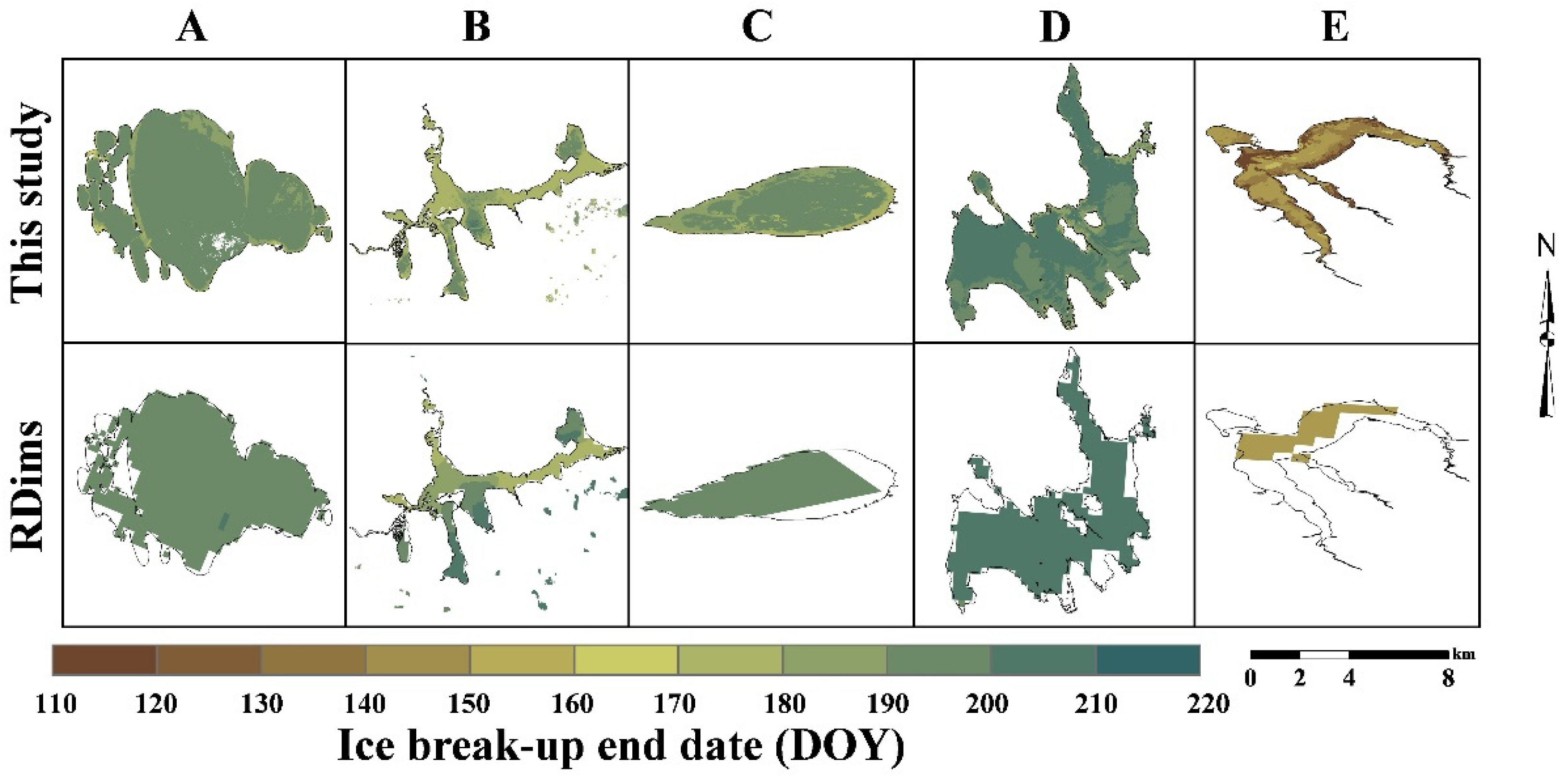
3.1. Assessment of the Refined Lake Extent

Table 1 shows the evaluation results of the lake extent refinement procedure. For the entire Pan-Arctic region, 45,532 lakes of 138,733 km2 were identified as the valid lake extent within the study area. In general, we observed the refined Pan-Arctic lake extent exhibits high accuracies, with a commission error, omission error, and F1 score of 6.7%, 6.8%, and 93.2%, respectively. In other words, the refinement procedure is effective for masking out irrelevant land covers (bare soil, vegetation, stable ice, and stable water) that were included in the original HydroLAKES dataset. We also found substantial accuracy variations across countries. Referring to the F1 score, the best performances are observed in Iceland (97.3%) and Norway (95.3%), followed by the USA (93.9%), Russia (91.2%), and Canada (88.3%). Moreover, in the USA and Canada, the accuracies measured by commission are slightly lower than those by omission, while in other countries the opposite trend (higher omission than commission) is observed. Referring to the lake area, we found that the majority of Arctic lakes are located in three countries, including Canada (30,325 lakes, 100,938 km2), Russia (11,495 lakes, 27,841 km2) and the USA (3647 lakes, 9905 km2), where the permafrost landscape is widely distributed. On the other hand, Norway and Iceland have tiny shares of the total lake area extent, primarily due to the smaller landmass of these two countries.
The discrepancy between the original HydroLAKES product and the refined lake extents can be attributed to two primary reasons: misclassification errors of the HydroLAKES dataset and changes in lake extents. Figure 4 displays three typical subsets (200 × 200 pixels for each), representing the diversity of Arctic lake and landscape characteristics. The lake shoreline polygons before and after the refinement were compared and analyzed. Subset 1 is located in Siberia, Russia, while Subsets 2 and 3 are located in Alaska, USA. In Case 1, HydroLAKES mistakenly identifies a cluster of pixels as a lake, which is actually a shaded region covered by shrubs. Such an omission error, however, is not observed in our refined output. In Case 2, both the results with and without the refinement procedure capture the overall pattern of the lake boundaries. However, differences still existed following a further look. Specifically, we observed a slight shrinking trend in the largest lake in the middle, which is correctly reflected in the refined shoreline result. Case 3 further shows a more extreme situation in which the majority of lake areas has been lost and replaced by new plants. Therefore, the refined lake extent used in this study is more reasonable than the original HydroLAKES product for lake ice BUE mapping.

3.2. Evaluation of Lake Ice-Off Phenology Mapping

We evaluated the estimated lake ice BUE map based on the RDsite and RDsat datasets. We found that our predictions and the actual BUE dates are overall in good agreement (Figure 5). Table 2 further displays the quantitative accuracy metrics. We found that the predicted outputs are more subject to positive bias errors, with ME values of 0.34 and 6.14 days for RDsite and RDsat, respectively, meaning a higher probability of a delay in the lake ice BUE date detection. Comparatively, our BUE predictions show a slightly better performance in matching RDsite than RDsat by all measures.
We further evaluated the performance of our proposed algorithm in estimating lake ice BUE using the RDims dataset. These results were summarized in the density plots using pixel and lake as the statistical unit, respectively (Figure 6). In general, we found that our predictions are generally consistent with those derived from the IMS time series, although the BUE difference is inherently variable within and among lakes. By forcing the intercept of the linear fit to zero [44], we found that our predictions show systematic underestimations (i.e., slope > 1.00 and ME < 0) with the IMS-based BUE. Specifically, at the pixel level our predictions explain 65% of the variations of RDims, while at the lake level 57% of the variation can be explained by the predicted BUE. Regarding MAE and RMSE, similar results were observed, indicating consistent performance across different spatial levels.
Figure 7 further compares lake ice BUE maps from RDims and our predictions by selecting five Arctic lakes, each of which represents one typical landscape. In general, we found that both mapping results correctly reflect the BUE variation within and among lakes, with BUE dates ranging from 110 to 220. Spatially, our BUE maps can provide more details over space and exhibit more consistent BUE patterns. Taking lake Taymyr (A) and lake Hall (D) as examples, the BUE difference between the lake center and lake shore is better captured by our predictions than those of RDims. Such a mapping performance enhancement is primarily due to the improved spatial resolution of Sentinel-2, which allows us to reveal the hidden patterns of BUE heterogeneity that would otherwise not be detected using coarse resolution products (e.g., IMS). Apart from the improvement in mapping accuracy, our 20 m BUE map is also associated with reduced uncertainty caused by the noise introduced by mixing pixels at the shoreline (e.g., lake Ozero Yarato (C) and lake Nanvaranak (E) in Figure 7), and is capable of offering more spatially continuous lake ice BUE estimates across the entire Arctic.

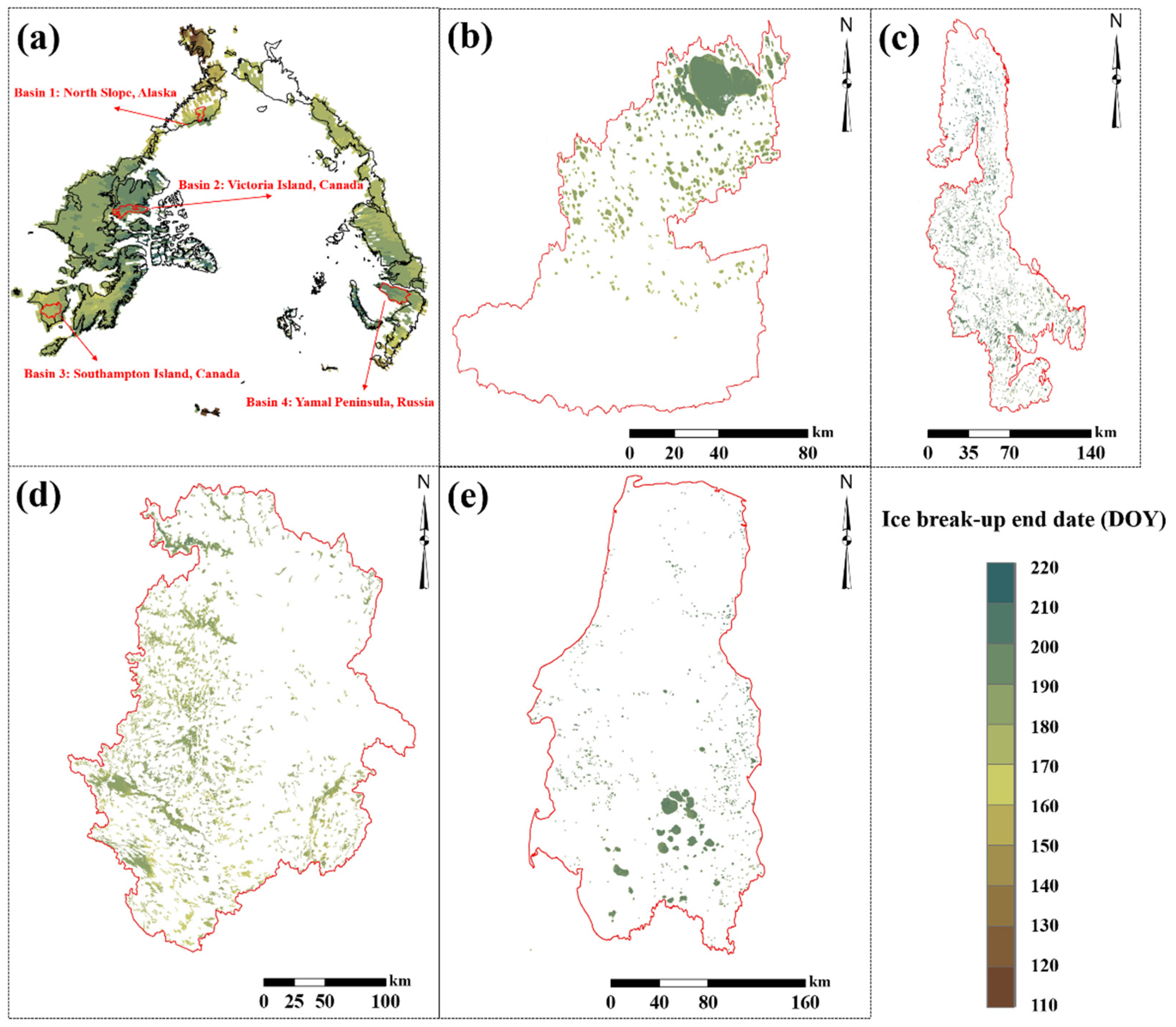
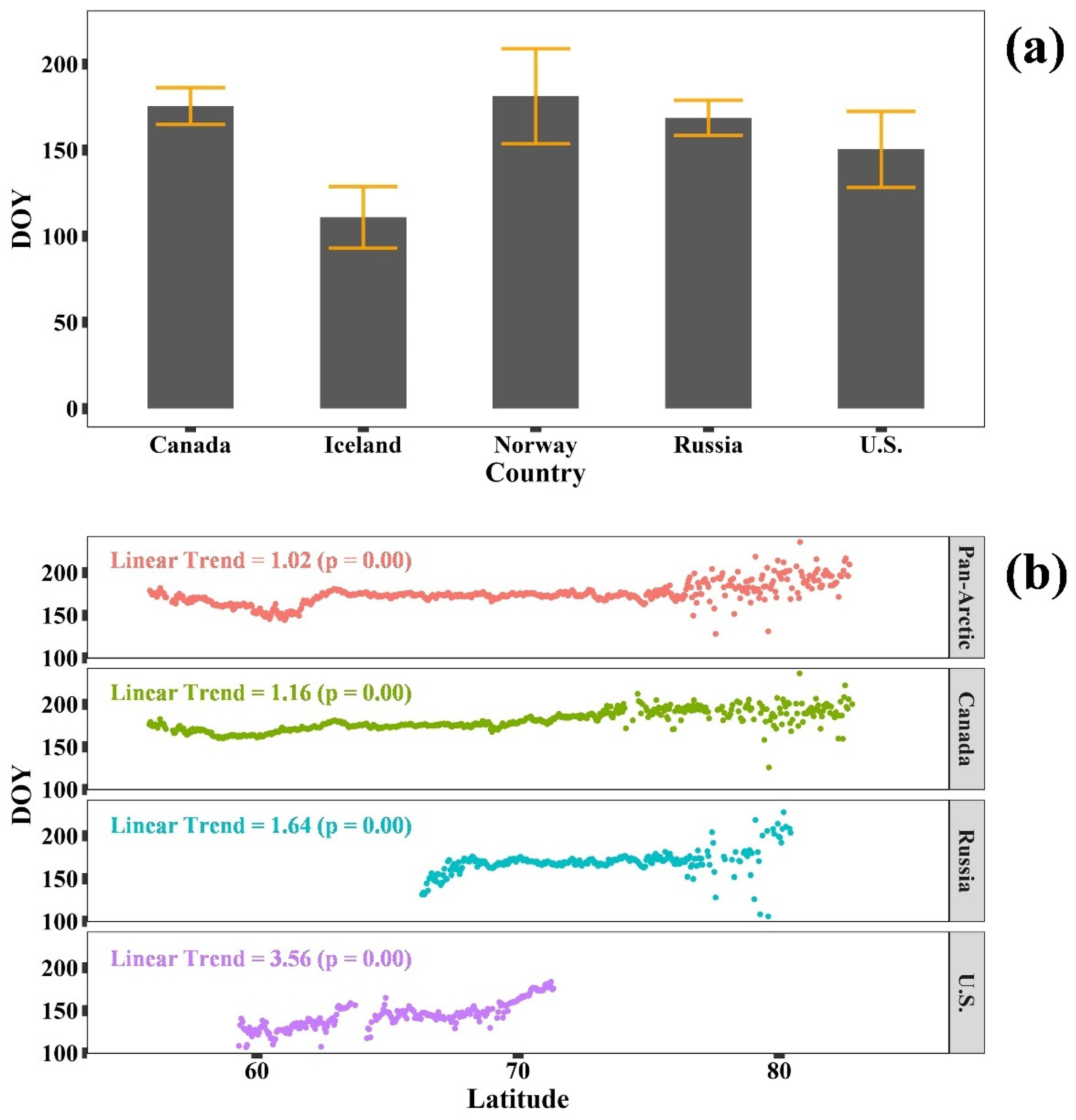
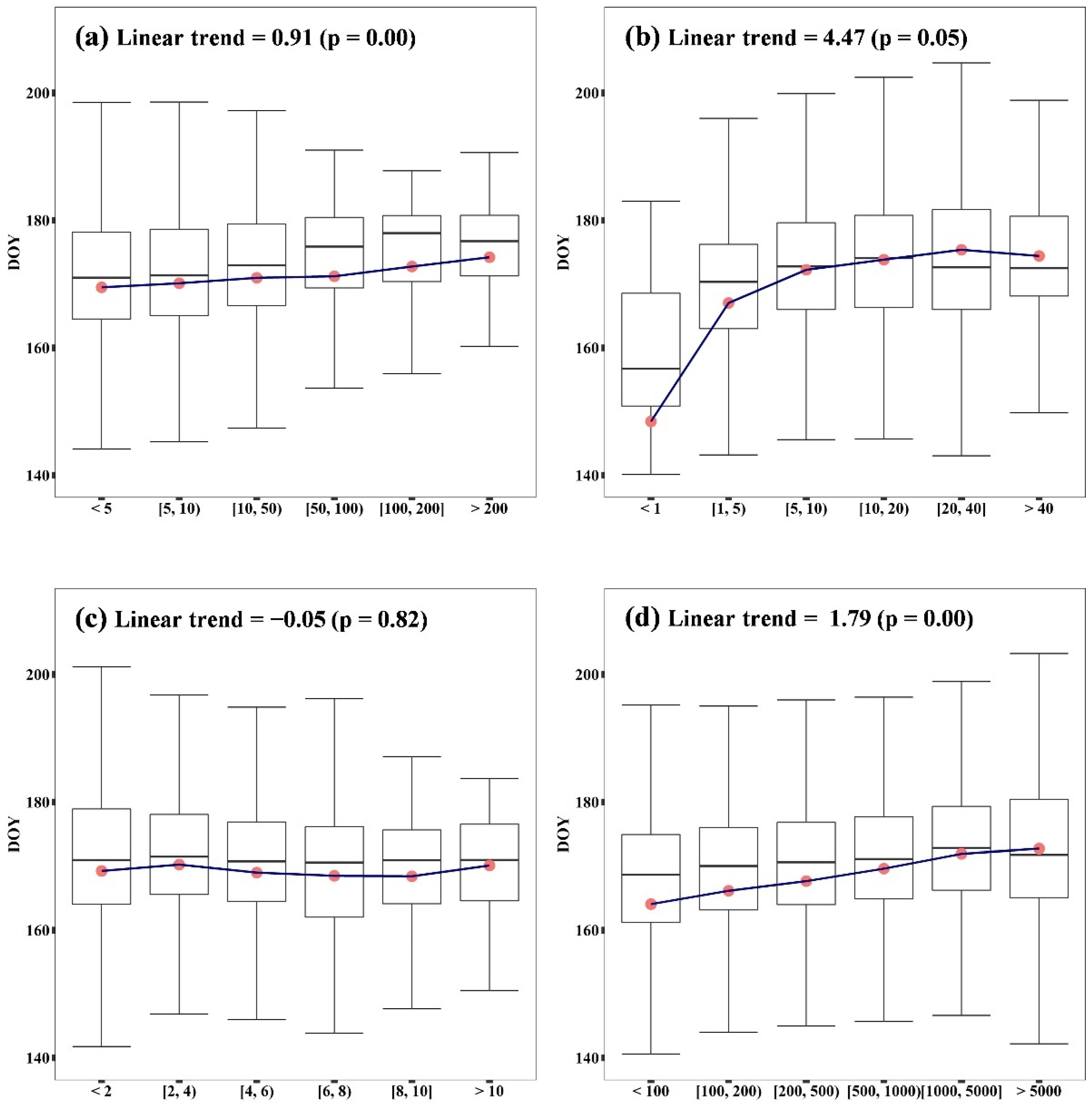
3.3. Spatial Pattern of Pan-Arctic Lake Ice BUE

Using the proposed approach, we calculated the Pan-Arctic lake ice BUE and mapped its distribution (Figure 8). Based on this map, we estimated that the average BUE of Pan-Arctic lakes for the year 2019 is 21 June (DOY = 172 ± 13.4 days, one standard deviation). Spatially, we found that the BUE distribution is strongly associated with latitudinal gradients. Earlier lake ice-off is observed in Iceland, Southwest Alaska, the Southampton Island of Canada, and some parts of Southern Siberia. Conversely, later clearing of lake ice is detected over relatively high latitudes, such as the Svalbard Archipelago of Norway, the Ellesmere Island of Canada, and the Severny Island of Russia. We also displayed finer-scale lake ice BUE mapping results by selecting four hydrological basins. In general, we found that small lakes have earlier ice BUE dates than large ones (see Basin 1 and Basin 3), though the magnitude of difference varies across basins. Similar with Figure 7, for some big lakes there exist discrepancies between the nearshore pixels and those located in the central lake areas.
We further divided the Pan-Arctic lake ice BUE map into countries, and the results are shown in Figure 9a. Regarding the average value of the BUE, we found that Norway exhibits the latest BUE date (181), followed by Canada (175), Russia (169), and the USA (150), respectively. In contrast, an earlier BUE estimation by our output is observed in Iceland (112). Overall, countries with greater lake concentrations are less subject to internal variability, as reflected by the lower standard deviations (error bar in Figure 9a). In particular, for Russia, Canada, Iceland, the USA, and Norway, the BUE standard deviations are ± 10.2, ± 10.7, ± 17.9, ± 22.1, and ± 27.6 days, respectively. Along latitude, all countries (except for Norway and Iceland) exhibit significant trends, together resulting in a linear slope of 1.02 days per degree for the Pan-Arctic (Figure 9b). Moreover, the latitudinal profile of Pan-Arctic lake ice BUE can be roughly divided into four phases by visual interpretation. There is a slight negative trend from 55°N to 62°N, followed by a dramatic increase from 62°N to 65°N, and a relatively stable sequence from 65°N to 78°N. Finally, the BUE is likely to increase from 78°N onward. At the country level, the greatest positive trend is detected in the USA, although its latitudinal range is limited (approximately from 59°N to 72°N). For Russia, relatively obvious increases are found in its southern and northern parts. The latitudinal profile of Canada exhibits the strongest agreement with the entire study area, indicating its prominent role in shaping the Pan-Arctic lake ice-off phenology.
To examine the sensitivity of the BUE to landscape parameters, we conducted an analysis of the influence of parameter change on BUE distribution at the lake level. These results are displayed and summarized in Figure 10. Except for shoreline development, we found that lake ice BUE is significantly impacted by the selected parameters, including lake area (p = 0.00), lake depth (p = 0.05), and residence time of the lake waters (p = 0.00). As suggested by previous studies [25,45], we demonstrated that bigger lakes are more likely to have later BUE dates and less internal variability than smaller lakes (Figure 10a). On the other hand, an overall later trend is also detected with lake depth increasing, with the most striking BUE change occurring at a lake depth of approximately 1 m (Figure 10b). Additionally, we found the BUE response to lake depth gradient is highly nonlinear, displaying a “saturation” phenomenon for deep lakes. Our analysis further indicates that the relationship between lake ice BUE and shoreline development is insignificant (p = 0.82, Figure 10c). Such a result, however, is different from that of several regional research studies, highlighting the impact of lake morphology on lake ice phenology [46,47]. Last but not least, we found a consistent and linear increase along the residence time profile (Figure 10d), suggesting that Arctic lakes with higher hydrologic connectivity tend to have earlier ice melting dates [48].

4. Discussion

Regulating many aspects of Arctic ecosystems, the spatial distribution of lake ice-off phenology is important for us to understand the earliest detected impacts of climatic warming [40,43,49,50]. However, the diversity of freshwater lakes, landscape heterogeneity, and varying weather conditions make fine-resolution Pan-Arctic lake ice BUE mapping a challenging task. In this study, we proposed a novel approach for per-pixel BUE identification based on Sentinel-2 constellation data. We examined the lake ice BUE mapping performance and found that the estimated results matched well with in situ measurements and existing microwave satellite records (Table 2, Figure 5, Figure 6 and Figure 7). The main advantages of the new approach are threefold. First, we confirmed the effectiveness of the SCL band of the Sentinel-2 Level 2A product for seasonal ice/water monitoring and incorporated it into our BUE identification approach. We showed that the refined lake extent can better reflect the shoreline boundaries than the original HydroLAKES dataset (Table 1, Figure 4); therefore, the errors caused by lake/land confusion can be greatly reduced or even eliminated. Second, we designed a “max-seg-difference” algorithm, which detects the abrupt change of the binary phenophase time series through temporal segmentation at the pixel level (Figure 3). Compared with commonly used threshold-based methods (e.g., [9,43]), the “max-seg-difference” algorithm is more robust and self-adaptive. As a result, it can be applied to various geographical environments without user intervention. Moreover, the use of phenophase information rather than initial satellite reflectance data has the potential of integrating more data types (e.g., SAR) for fine-resolution lake ice BUE mapping. Finally, we employed the GEE platform to run the full process under the proposed approach, which enables us to apply BUE mapping over a large spatial extent in an effective and efficient manner.
To the best of our knowledge, this study provides the first spatially continuous map of Pan-Arctic lake ice BUE at a 20 m resolution, which can facilitate ongoing efforts to understand the changing Arctic ecosystems. Finer spatial resolution BUE information is not only statistically beneficial for more accurate estimation, but also allows us to reveal the hidden patterns of lake ice melting that would otherwise not be detected using coarse resolution products [15,20]. For example, we found that the nearshore lake ice is likely to melt earlier than that distributed in the central lake area (Figure 7 and Figure 8). Consistent with some previous studies [15,24], our lake ice BUE estimates exhibited an overall later trend with latitudinal gradients across the Pan-Arctic region. However, the magnitude of the latitudinal BUE shift is unevenly distributed (Figure 9), highlighting the complex suite of climatic and ecological forces that can play roles in spring lake ice melting. With an improved resolution, the new BUE map is particularly valuable for monitoring spring ice melting of small lakes, which constitutes the majority of total Arctic lake populations that are most vulnerable to climate change [27]. Theoretically, a small lake is fundamentally different from a big one in thermodynamic processes [25]. Our results confirmed this discrepancy by showing that the BUE date tends to occur later with increasing lake areas and lake depths (Figure 10a,b). Since small lakes are commonly ignored in previous Arctic lake ice phenology studies, reanalysis may be needed using finer-resolution data to clarify the existing findings of Arctic lake ice-off timing dynamics over space and time. We noted an insignificant change in lake ice BUE along the shoreline development profile (Figure 10c), reflecting the internal heterogeneity that obscures the expected effects of lake morphology. For example, within the lake extent, its shoreline topography can be very different. This may influence the wind speed and direction, both of which are drivers of initial ice breaking in early spring [25]. Additionally, our study also provides observational evidence of the hydrological drivers in joint-shaping BUE diversity through connectivity (Figure 10d). Water bodies with high hydrologic connectivity and short residence times are more subject to heat exchange, thus taking fewer days to become ice free in spring [25].
While presenting substantial confidence regarding the Pan-Arctic mapping of fine-resolution lake ice BUE, the proposed approach has limitations and uncertainties. In this study, we selected twin Sentinel-2 satellites as the base data source because of its relatively high spatial and temporal resolutions. With a temporal interval of 5 days, the reconstructed Sentinel-2 composite performed well in general for extracting Pan-Arctic BUE information. Nevertheless, cloud obscuration will lower the actual revisit frequency, making our approach less effective in tracking sub-seasonal variations in lake ice extent. In this sense, the increasing availability of miniature satellites in low Earth orbit, known as CubeSats (e.g., Planet and RapidEye), may offer added value for the timely and accurate estimation of lake ice phenology [5,49]. The derivation of accurate lake extent has always been a critical constraint on ice BUE mapping. In this study, the depicting of lake extent mainly relies on the HydroLAKES dataset, even after a refinement procedure was conducted. The errors of incorrect lake shoreline boundaries will be eventually propagated to the final BUE outputs, and make our estimates less informative. The “max-seg-difference” algorithm depends heavily on the accuracy of SCL, which inevitably contains classification errors. A recent study showed that there is room for improvement in the current scene classification algorithm by ESA [38]. Hence, a better BUE mapping performance of our approach can be expected once the new version of the SCL product is ready for use.
This study has both methodological and practical implications for future endeavors on Arctic-wide lake ice monitoring. By further including SAR time series data, the proposed approach can be extended to track the ice freeze-up process, which is equally important in understanding the Arctic lake system. Using this study as the baseline, the spatial-temporal dynamics of Arctic lake ice phenology can be quantified, making it possible to examine their drivers and project future changes. Moreover, the fine-resolution lake ice BUE map will benefit a variety of scientific research on Arctic ecosystems. For example, lakes are considered a major source of atmospheric methane (CH4) [11,12], and the timing of ice-off can affect the annual quantity of methane emitted from water to the atmosphere [17]. Finally, we emphasize the necessity of more comprehensive, spatially representative databases that can provide in situ ice phenology records to support model development and validation. So far, there are many lakes where the measurements are discontinued and outdated [8]. We expect this data gap can be filled by new and collaborative programs in the near future.

5. Conclusions

Accurately mapping lake ice-off phenology is essential for us to understand a changing Arctic. In this study, we developed a novel approach for fine-resolution BUE mapping with the use of dense Sentinel-2 time series data via the GEE platform. Experimental results in 45,532 lakes across the Arctic reveal the feasibility of this approach. From the estimated Pan-Arctic lake ice BUE map, four major conclusions can be drawn. First, the Sentinel-2 SCL time series dataset shows great potential in monitoring the sub-seasonal dynamics of ice/water coverage with high spatial (20 m) and temporal (5 day) resolutions, which can facilitate the fine-scale detection of lake ice melting. Second, the utilization of a binary phenophase profile rather than original spectral signatures can reduce data uncertainties, making the “max-seg-difference” algorithm self-adaptive for per-pixel BUE identification and efficient for large area application. Third, the mapped lake ice-off phenology exhibits gradients along the latitude profile and lake characteristics, indicating the joint control of climate and local landscapes in determining Arctic lake ice melting. Finally, we concluded that the new approach provided an improved estimate of Pan-Arctic lake ice BUE, which is expected to enlighten the continuing endeavor for achieving sustainable development goals. Future studies can consider environmental characteristics that were not explored in this study, such as lake ice quality, human footprint, and their impacts on Arctic lake ice BUE. Additionally, SAR satellite data hold potential in capturing ice melting/freezing information without the influence of unfavorable weather conditions. They can be thus combined with optical imagery for providing a refined characterization of Arctic lake ice phenology as well as its multi-decadal dynamics.

Author Contributions

Conceptualization, C.L., F.H. and X.C.; methodology, C.L. and H.H.; software, C.L. and Z.Z.; validation, C.L. and Z.Z.; formal analysis, C.L.; investigation, C.L. and Z.Z.; writing—original draft preparation, C.L.; writing—review and editing, C.L., H.H., F.H. and X.C.; visualization, C.L.; supervision, X.C. All authors have read and agreed to the published version of the manuscript.

Funding

This research was funded by the National Key R&D Program of China (No. 2019YFC1509104, No. 2018YFC1407103) and Innovation Group Project of Southern Marine Science and Engineering Guangdong Laboratory (Zhuhai) (No. 311021008).

Data Availability Statement

The Pan-Arctic lake ice-off phenology map for the year 2019 at 20 m resolution is publicly available from the corresponding author on reasonable request.

Acknowledgments

We are grateful to the European Space Agency for providing the Sentinel-2 data, European Centre for Medium-Range Weather Forecasts for providing the ERA5 data, World Wildlife Fund for providing the HydroLAKES dataset, and the Finnish Environmental Institute for providing in situ lake ice phenology measurements. This work would not have been possible without the computing support from the Google Earth Engine platform, which is a cloud-based platform for planetary-scale geospatial analysis. We would also like to thank Qi Zhang and Shiqi Tao for their assistance in manuscript editing.

Conflicts of Interest

The authors declare no conflict of interest.

References

  1. Paltan, H.; Dash, J.; Edwards, M. A Refined Mapping of Arctic Lakes Using Landsat Imagery. Int. J. Remote Sens. 2015, 36, 5970–5982. [Google Scholar] [CrossRef] [Green Version]
  2. Muster, S.; Roth, K.; Langer, M.; Lange, S.; Cresto Aleina, F.; Bartsch, A.; Morgenstern, A.; Grosse, G.; Jones, B.; Sannel, A.B.K.; et al. PeRL: A Circum-Arctic Permafrost Region Pond and Lake Database. Earth Syst. Sci. Data 2017, 9, 317–348. [Google Scholar] [CrossRef] [Green Version]
  3. Nitze, I.; Grosse, G.; Jones, B.M.; Romanovsky, V.E.; Boike, J. Remote Sensing Quantifies Widespread Abundance of Permafrost Region Disturbances across the Arctic and Subarctic. Nat. Commun. 2018, 9, 5423. [Google Scholar] [CrossRef]
  4. Olefeldt, D.; Hovemyr, M.; Kuhn, M.A.; Bastviken, D.; Bohn, T.J.; Connolly, J.; Crill, P.; Euskirchen, E.S.; Finkelstein, S.A.; Genet, H.; et al. The Boreal-Arctic Wetland and Lake Dataset (BAWLD). Earth Syst. Sci. Data Discuss. 2021, 2021, 1–40. [Google Scholar] [CrossRef]
  5. Cooley, S.W.; Smith, L.C.; Ryan, J.C.; Pitcher, L.H.; Pavelsky, T.M. Arctic-Boreal Lake Dynamics Revealed Using CubeSat Imagery. Geophys. Res. Lett. 2019, 46, 2111–2120. [Google Scholar] [CrossRef]
  6. Newton, A.M.W.; Mullan, D. Climate Change and Northern Hemisphere Lake and River Ice Phenology. Cryosphere Discuss. 2020, 2020, 1–60. [Google Scholar] [CrossRef]
  7. Surdu, C.M.; Duguay, C.R.; Fernández Prieto, D. Evidence of Recent Changes in the Ice Regime of Lakes in the Canadian High Arctic from Spaceborne Satellite Observations. Cryosphere 2016, 10, 941–960. [Google Scholar] [CrossRef] [Green Version]
  8. Weber, H.; Riffler, M.; Nõges, T.; Wunderle, S. Lake Ice Phenology from AVHRR Data for European Lakes: An Automated Two-Step Extraction Method. Remote Sens. Environ. 2016, 174, 329–340. [Google Scholar] [CrossRef]
  9. Zhang, S.; Pavelsky, T.M. Remote Sensing of Lake Ice Phenology across a Range of Lakes Sizes, ME, USA. Remote Sens. 2019, 11, 1718. [Google Scholar] [CrossRef] [Green Version]
  10. Cory, R.M.; Ward, C.P.; Crump, B.C.; Kling, G.W. Sunlight Controls Water Column Processing of Carbon in Arctic Fresh Waters. Science 2014, 345, 925. [Google Scholar] [CrossRef]
  11. Engram, M.; Anthony, K.W.; Meyer, F.J.; Grosse, G. Synthetic Aperture Radar (SAR) Backscatter Response from Methane Ebullition Bubbles Trapped by Thermokarst Lake Ice. Can. J. Remote Sens. 2013, 38, 667–682. [Google Scholar] [CrossRef]
  12. Engram, M.; Walter Anthony, K.M.; Sachs, T.; Kohnert, K.; Serafimovich, A.; Grosse, G.; Meyer, F.J. Remote Sensing Northern Lake Methane Ebullition. Nat. Clim. Chang. 2020, 10, 511–517. [Google Scholar] [CrossRef]
  13. Rey, D.M.; Walvoord, M.; Minsley, B.; Rover, J.; Singha, K. Investigating Lake-Area Dynamics across a Permafrost-Thaw Spectrum Using Airborne Electromagnetic Surveys and Remote Sensing Time-Series Data in Yukon Flats, Alaska. Environ. Res. Lett. 2019, 14, 025001. [Google Scholar] [CrossRef]
  14. Ruan, Y.; Zhang, X.; Xin, Q.; Qiu, Y.; Sun, Y. Prediction and Analysis of Lake Ice Phenology Dynamics Under Future Climate Scenarios Across the Inner Tibetan Plateau. J. Geophys. Res. Atmos. 2020, 125, e2020JD033082. [Google Scholar] [CrossRef]
  15. Dauginis, A.A.; Brown, L.C. Recent Changes in Pan-Arctic Sea Ice, Lake Ice, and Snow on/off Timing. Cryosphere Discuss. 2021, 2021, 1–35. [Google Scholar] [CrossRef]
  16. Brown, L.C.; Duguay, C.R. Modelling Lake Ice Phenology with an Examination of Satellite-Detected Subgrid Cell Variability. Adv. Meteorol. 2012, 2012, 529064. [Google Scholar] [CrossRef] [Green Version]
  17. Yang, X.; Pavelsky, T.M.; Allen, G.H. The Past and Future of Global River Ice. Nature 2020, 577, 69–73. [Google Scholar] [CrossRef]
  18. Duguay, C.R.; Bernier, M.; Gauthier, Y.; Kouraev, A. Remote sensing of lake and river ice. In Remote Sensing of the Cryosphere; John Wiley & Sons, Ltd.: Hoboken, NJ, USA, 2015; pp. 273–306. ISBN 978-1-118-36890-9. [Google Scholar]
  19. Che, T.; Li, X.; Jin, R. Monitoring the Frozen Duration of Qinghai Lake Using Satellite Passive Microwave Remote Sensing Low Frequency Data. Chin. Sci. Bull. 2009, 54, 2294–2299. [Google Scholar] [CrossRef]
  20. Kang, K.-K.; Duguay, C.R.; Howell, S.E.L. Estimating Ice Phenology on Large Northern Lakes from AMSR-E: Algorithm Development and Application to Great Bear Lake and Great Slave Lake, Canada. Cryosphere 2012, 6, 235–254. [Google Scholar] [CrossRef] [Green Version]
  21. Xiong, C.; Lei, Y.; Qiu, Y. Contrasting Lake Ice Phenology Changes in the Qinghai-Tibet Plateau Revealed by Remote Sensing. IEEE Geosci. Remote Sens. Lett. 2020, 1–5. [Google Scholar] [CrossRef]
  22. Murfitt, J.; Duguay, C.R. Assessing the Performance of Methods for Monitoring Ice Phenology of the World’s Largest High Arctic Lake Using High-Density Time Series Analysis of Sentinel-1 Data. Remote Sens. 2020, 12, 382. [Google Scholar] [CrossRef] [Green Version]
  23. Yang, Q.; Song, K.; Wen, Z.; Hao, X.; Fang, C. Recent Trends of Ice Phenology for Eight Large Lakes Using MODIS Products in Northeast China. Int. J. Remote Sens. 2019, 40, 5388–5410. [Google Scholar] [CrossRef]
  24. Šmejkalová, T.; Edwards, M.E.; Dash, J. Arctic Lakes Show Strong Decadal Trend in Earlier Spring Ice-Out. Sci. Rep. 2016, 6, 38449. [Google Scholar] [CrossRef] [PubMed]
  25. Sharma, S.; Meyer, M.F.; Culpepper, J.; Yang, X.; Hampton, S.; Berger, S.A.; Brousil, M.R.; Fradkin, S.C.; Higgins, S.N.; Jankowski, K.J.; et al. Integrating Perspectives to Understand Lake Ice Dynamics in a Changing World. J. Geophys. Res. Biogeosci. 2020, 125, e2020JG005799. [Google Scholar] [CrossRef]
  26. Scott, K.A.; Xu, L.; Pour, H.K. Retrieval of Ice/Water Observations from Synthetic Aperture Radar Imagery for Use in Lake Ice Data Assimilation. J. Gt. Lakes Res. 2020, 46, 1521–1532. [Google Scholar] [CrossRef]
  27. Mishra, V.; Cherkauer, K.A.; Bowling, L.C.; Huber, M. Lake Ice Phenology of Small Lakes: Impacts of Climate Variability in the Great Lakes Region. Glob. Planet. Chang. 2011, 76, 166–185. [Google Scholar] [CrossRef]
  28. Walker, D.A.; Reynolds, M.K.; Daniëls, F.J.A.; Einarsson, E.; Elvebakk, A.; Gould, W.A.; Katenin, A.E.; Kholod, S.S.; Markon, C.J.; Melnikov, E.S.; et al. The Circumpolar Arctic Vegetation Map. J. Veg. Sci. 2005, 16, 267–282. [Google Scholar] [CrossRef]
  29. Raynolds, M.K.; Walker, D.A.; Balser, A.; Bay, C.; Campbell, M.; Cherosov, M.M.; Daniëls, F.J.A.; Eidesen, P.B.; Ermokhina, K.A.; Frost, G.V.; et al. A Raster Version of the Circumpolar Arctic Vegetation Map (CAVM). Remote Sens. Environ. 2019, 232, 111297. [Google Scholar] [CrossRef]
  30. Messager, M.L.; Lehner, B.; Grill, G.; Nedeva, I.; Schmitt, O. Estimating the Volume and Age of Water Stored in Global Lakes Using a Geo-Statistical Approach. Nat. Commun. 2016, 7, 13603. [Google Scholar] [CrossRef]
  31. Liang, Y.-L.; Colgan, W.; Lv, Q.; Steffen, K.; Abdalati, W.; Stroeve, J.; Gallaher, D.; Bayou, N. A Decadal Investigation of Supraglacial Lakes in West Greenland Using a Fully Automatic Detection and Tracking Algorithm. Remote Sens. Environ. 2012, 123, 127–138. [Google Scholar] [CrossRef] [Green Version]
  32. Gorelick, N.; Hancher, M.; Dixon, M.; Ilyushchenko, S.; Thau, D.; Moore, R. Google Earth Engine: Planetary-Scale Geospatial Analysis for Everyone. Big Remote. Sensed Data Tools Appl. Exp. 2017, 202, 18–27. [Google Scholar] [CrossRef]
  33. Louis, J.; Pflug, B.; Main-Knorn, M.; Debaecker, V.; Mueller-Wilm, U.; Iannone, R.Q.; Cadau, E.G.; Boccia, V.; Gascon, F. Sentinel-2 Global Surface Reflectance Level-2a Product Generated with Sen2Cor. In Proceedings of the IGARSS 2019—2019 IEEE International Geoscience and Remote Sensing Symposium, Yokohama, Japan, 28 July–2 August 2019; pp. 8522–8525. [Google Scholar]
  34. Smith, L.C.; Sheng, Y.; MacDonald, G.M.; Hinzman, L.D. Disappearing Arctic Lakes. Science 2005, 308, 1429. [Google Scholar] [CrossRef] [Green Version]
  35. Pickens, A.H.; Hansen, M.C.; Hancher, M.; Stehman, S.V.; Tyukavina, A.; Potapov, P.; Marroquin, B.; Sherani, Z. Mapping and Sampling to Characterize Global Inland Water Dynamics from 1999 to 2018 with Full Landsat Time-Series. Remote Sens. Environ. 2020, 243, 111792. [Google Scholar] [CrossRef]
  36. Dong, J.; Xiao, X.; Menarguez, M.A.; Zhang, G.; Qin, Y.; Thau, D.; Biradar, C.; Moore, B., III. Mapping Paddy Rice Planting Area in Northeastern Asia with Landsat 8 Images, Phenology-Based Algorithm and Google Earth Engine. Remote Sens. Environ. 2016, 185, 142–154. [Google Scholar] [CrossRef] [Green Version]
  37. Chen, B.; Xiao, X.; Li, X.; Pan, L.; Doughty, R.; Ma, J.; Dong, J.; Qin, Y.; Zhao, B.; Wu, Z.; et al. A Mangrove Forest Map of China in 2015: Analysis of Time Series Landsat 7/8 and Sentinel-1A Imagery in Google Earth Engine Cloud Computing Platform. ISPRS J. Photogramm. Remote Sens. 2017, 131, 104–120. [Google Scholar] [CrossRef]
  38. Raiyani, K.; Gonçalves, T.; Rato, L.; Salgueiro, P.; Marques da Silva, J.R. Sentinel-2 Image Scene Classification: A Comparison between Sen2Cor and a Machine Learning Approach. Remote Sens. 2021, 13, 300. [Google Scholar] [CrossRef]
  39. Zhu, Z.; Zhang, J.; Yang, Z.; Aljaddani, A.H.; Cohen, W.B.; Qiu, S.; Zhou, C. Continuous Monitoring of Land Disturbance Based on Landsat Time Series. Time Ser. Anal. High Spat. Resolut. Imag. 2020, 238, 111116. [Google Scholar] [CrossRef]
  40. Arp, C.D.; Jones, B.M.; Grosse, G. Recent Lake Ice-out Phenology within and among Lake Districts of Alaska, U.S.A. Limnol. Oceanogr. 2013, 58, 2013–2028. [Google Scholar] [CrossRef]
  41. Liu, C.; Zhang, Q.; Tao, S.; Qi, J.; Ding, M.; Guan, Q.; Wu, B.; Zhang, M.; Nabil, M.; Tian, F.; et al. A New Framework to Map Fine Resolution Cropping Intensity across the Globe: Algorithm, Validation, and Implication. Remote Sens. Environ. 2020, 251, 112095. [Google Scholar] [CrossRef]
  42. Duguay, C.R.; Prowse, T.D.; Bonsal, B.R.; Brown, R.D.; Lacroix, M.P.; Ménard, P. Recent Trends in Canadian Lake Ice Cover. Hydrol. Process. 2006, 20, 781–801. [Google Scholar] [CrossRef]
  43. Du, J.; Kimball, J.S.; Duguay, C.; Kim, Y.; Watts, J.D. Satellite Microwave Assessment of Northern Hemisphere Lake Ice Phenology from 2002 to 2015. Cryosphere 2017, 11, 47–63. [Google Scholar] [CrossRef] [Green Version]
  44. Liu, C.; Zhang, Q.; Luo, H.; Qi, S.; Tao, S.; Xu, H.; Yao, Y. An Efficient Approach to Capture Continuous Impervious Surface Dynamics Using Spatial-Temporal Rules and Dense Landsat Time Series Stacks. Remote Sens. Environ. 2019, 229, 114–132. [Google Scholar] [CrossRef]
  45. Kirillin, G.; Leppäranta, M.; Terzhevik, A.; Granin, N.; Bernhardt, J.; Engelhardt, C.; Efremova, T.; Golosov, S.; Palshin, N.; Sherstyankin, P.; et al. Physics of Seasonally Ice-Covered Lakes: A Review. Aquat. Sci. 2012, 74, 659–682. [Google Scholar] [CrossRef]
  46. Williams, G.; Layman, K.L.; Stefan, H.G. Dependence of Lake Ice Covers on Climatic, Geographic and Bathymetric Variables. Cold Reg. Sci. Technol. 2004, 40, 145–164. [Google Scholar] [CrossRef]
  47. Magee, M.R.; Wu, C.H. Effects of Changing Climate on Ice Cover in Three Morphometrically Different Lakes. Hydrol. Process. 2017, 31, 308–323. [Google Scholar] [CrossRef]
  48. Beltaos, S.; Prowse, T. River-Ice Hydrology in a Shrinking Cryosphere. Hydrol. Process. 2009, 23, 122–144. [Google Scholar] [CrossRef]
  49. Cooley, S.W.; Smith, L.C.; Stepan, L.; Mascaro, J. Tracking Dynamic Northern Surface Water Changes with High-Frequency Planet CubeSat Imagery. Remote Sens. 2017, 9, 1306. [Google Scholar] [CrossRef] [Green Version]
  50. Sharma, S.; Blagrave, K.; Magnuson, J.J.; O’Reilly, C.M.; Oliver, S.; Batt, R.D.; Magee, M.R.; Straile, D.; Weyhenmeyer, G.A.; Winslow, L.; et al. Widespread loss of lake ice around the Northern Hemisphere in a warming world. Nat. Clim. Chang. 2019, 9, 227–231. [Google Scholar] [CrossRef]
Figure 1. Overview of the study area. (a) Spatial coverage of the study area; (b) distribution of lake concentration, calculated as the percent area covered by lakes within a 25 km × 25 km grid; (c) distribution of the Sentinel-2 average revisit interval (day) within the study period (i.e., from 1 February to 1 September 2019).
Remotesensing 13 02742 g001
Figure 2. Flow chart of the lake ice BUE mapping proposed in this study.
Remotesensing 13 02742 g002
Figure 3. Illustration of the proposed “max-seg-difference” algorithm for BUE identification.
Remotesensing 13 02742 g003
Figure 4. Three typical subsets showing lake shorelines before and after the refinement procedure. The background maps are Sentinel-2 images (shortwave infrared, near infrared, and red bands are displayed in as red, green, and blue layers) acquired on 18 July 2019 for Subset 1 and on 24 July 2019 for Subsets 2–3, respectively.
Remotesensing 13 02742 g004
Figure 5. Box plots of the observed and predicted lake ice BUE dates using in situ observations (RDsite) and sample points from satellite visual interpretation (RDsat).
Remotesensing 13 02742 g005
Figure 6. Density plots showing the relationships between the predicted and RDims BUE dates using pixel (a) and lake (b) as the statistical unit. The red line represents the linear fit with the intercept forced to 0.
Remotesensing 13 02742 g006
Figure 7. Comparison of BUE maps for five Arctic lakes. (AE) represent lake Taymyr (Russia), lake Teshekpuk (U.S.), lake Ozero Yarato (Russia), lake Hall (Canada), and lake Nanvaranak (U.S.), respectively.
Remotesensing 13 02742 g007
Figure 8. (a) Pan-Arctic lake ice BUE map for the year 2019 at a 25 km × 25 km tile scale. Four hydrological basins are highlighted for visual display at a 20 m spatial resolution, including (b) North Slope, (c) Victoria Island, (d) Southampton Island, and (e) Yamal Peninsula.
Remotesensing 13 02742 g008
Figure 9. Geographical distribution of Pan-Arctic lake ice BUE. (a) Country-level statistics; (b) latitudinal profile, derived with an interval of 500 m.
Remotesensing 13 02742 g009
Figure 10. Characteristics of the Pan-Arctic lake ice BUE given (a) lake area (km2); (b) lake depth (m); (c) shoreline development, measured as the ratio between the shoreline length and the circumference of a circle with the same area; (d) residence time of the lake waters (day). The linear trend was calculated using the group-aggregated parameter–BUE pair, and the red point denotes the average value of each data group along the x-axis.
Remotesensing 13 02742 g010
Table 1. Evaluation of the refined lake extent.
RegionCommission (%) Omission (%)F1 Score (%)Refined Lake NumberRefined Lake Area (km2)
Canada17.35.388.330,325100,938
Iceland1.34.097.386
Norway2.76.795.35743
Russia5.312.0 91.211,49527,841
USA8.04.293.936479905
Pan-Arctic6.76.893.245,532138,733
Table 2. Error metrics of the predicted BUE results using RDsite and RDsat (unit: day).
Number of ObservationsMEMAERMSE
RDsite290.346.557.40
RDsat2346.147.799.92
Publisher’s Note: MDPI stays neutral with regard to jurisdictional claims in published maps and institutional affiliations.

