Abstract
Accurate and efficient burned area mapping and monitoring are fundamental for environmental applications. Studies using Landsat time series for burned area mapping are increasing and popular. However, the performance of burned area mapping with different spectral indices and Landsat time series has not been evaluated and compared. This study compares eleven spectral indices for burned area detection in the savanna area of southern Burkina Faso using Landsat data ranging from October 2000 to April 2016. The same reference data are adopted to assess the performance of different spectral indices. The results indicate that Burned Area Index (BAI) is the most accurate index in burned area detection using our method based on harmonic model fitting and breakpoint identification. Among those tested, fire-related indices are more accurate than vegetation indices, and Char Soil Index (CSI) performed worst. Furthermore, we evaluate whether combining several different spectral indices can improve the accuracy of burned area detection. According to the results, only minor improvements in accuracy can be attained in the studied environment, and the performance depended on the number of selected spectral indices.
1. Introduction
The African savanna frequently experiences extensive fires every year, as thousands of square kilometers are burned, making an important contribution to the total global burned area [1]. Fire is recognized as an important feature in savanna ecosystems, as it plays a key role in vegetation succession, carbon cycle, biodiversity, and land management [2]. Therefore, timely and accurate mapping of burned areas is essential for fire management, climate modeling, and environmental applications. The rapid development of remote sensing technology provides convenient and effective methods for burned area mapping from regional to global scale. Previously, coarse spatial resolution data from Advanced Very High Resolution Radiometer (AVHRR), Moderate Resolution Imaging Spectroradiometer (MODIS), or SPOT VEGETATION images have been widely used for monitoring burned areas [3]. However, the resolution of these sensors is too coarse to identify small burn patches and their dynamics on a regional scale. The increasing availability of medium spatial resolution satellite images, such as Landsat, is a valuable source of information for more accurate detection of the burned areas at local and regional scales.
A variety of methods have been developed for burned area monitoring and mapping using remote sensing data, including threshold-based method with spectral indices [4], supervised image classification, such as decision trees classification [5], artificial neural networks [6], logistic regression [2], principal component analysis [7], region growing [8], and spectral mixture analysis [9]. Many burned area mapping methods use spectral indices based on post-fire images or pre-fire and post-fire images to identify burned areas and separate those from other land cover categories and states, due to their simplicity and efficiency. Vegetation index and fire index are two kinds of spectral indices that are widely applied for burned area detection. Normalized Difference Vegetation Index (NDVI) is a popular vegetation index that is used to discriminate between the burned and unburned areas, due to its strong sensitivity to vegetation changes. There are numerous modifications of NDVI that have been developed to reduce atmospheric sensitivity and background variability and successfully applied in burned area detection, including the Global Environmental Monitoring Index (GEMI), the Soil-Adjusted Vegetation Index (SAVI), and the Enhanced Vegetation Index (EVI) [10]. Some fire indices are specifically designed and developed to be sensitive to post-fire spectral signals, such as the Normalized Burned Ratio (NBR), the Burned Area Index (BAI), and the Char Soil Index (CSI) [11].
The method based on image comparison by differencing the post-fire and pre-fire images with spectral indices is frequently applied for burned area detection, and achieved satisfactory results [12]. However, this method is constrained by the limited availability of cloud-free images, as well as challenges related to image-to-image normalization. With free and open access to the Landsat archive, Landsat time series data have been increasingly utilized for burned area detection and evaluation. Goodwin and Collett [13] proposed a method with Landsat time series data, including outlier identification caused by burned vegetation using near-infrared and mid-infrared spectral bands, region growing segmentation, and classification tree to distinguish burned area from other changes. Hawbaker et al. [14] used machine learning, thresholding, and region growing methods to identify burned areas with Landsat time series data using spectral band NBR. Liu et al. [15] developed an approach for mapping annual burned areas using a harmonic model fitting with BAI time series and breakpoint identification in Landsat time series. However, the sensitivity of different spectral indices on discriminating burned and unburned areas using Landsat time series has not been studied.
In this paper, our objective was to explore and evaluate the effect of using various spectral indices based on Landsat time series on the performance of burned area detection. To accomplish this goal, we used all available Landsat images between 2000 and 2016 in savannas of southern Burkina Faso for mapping burned areas. Furthermore, we tested whether fusion of burned area detections based on several spectral indices can improve accuracy.
2. Materials and Methods
2.1. Study Area and Remote Sensing Data
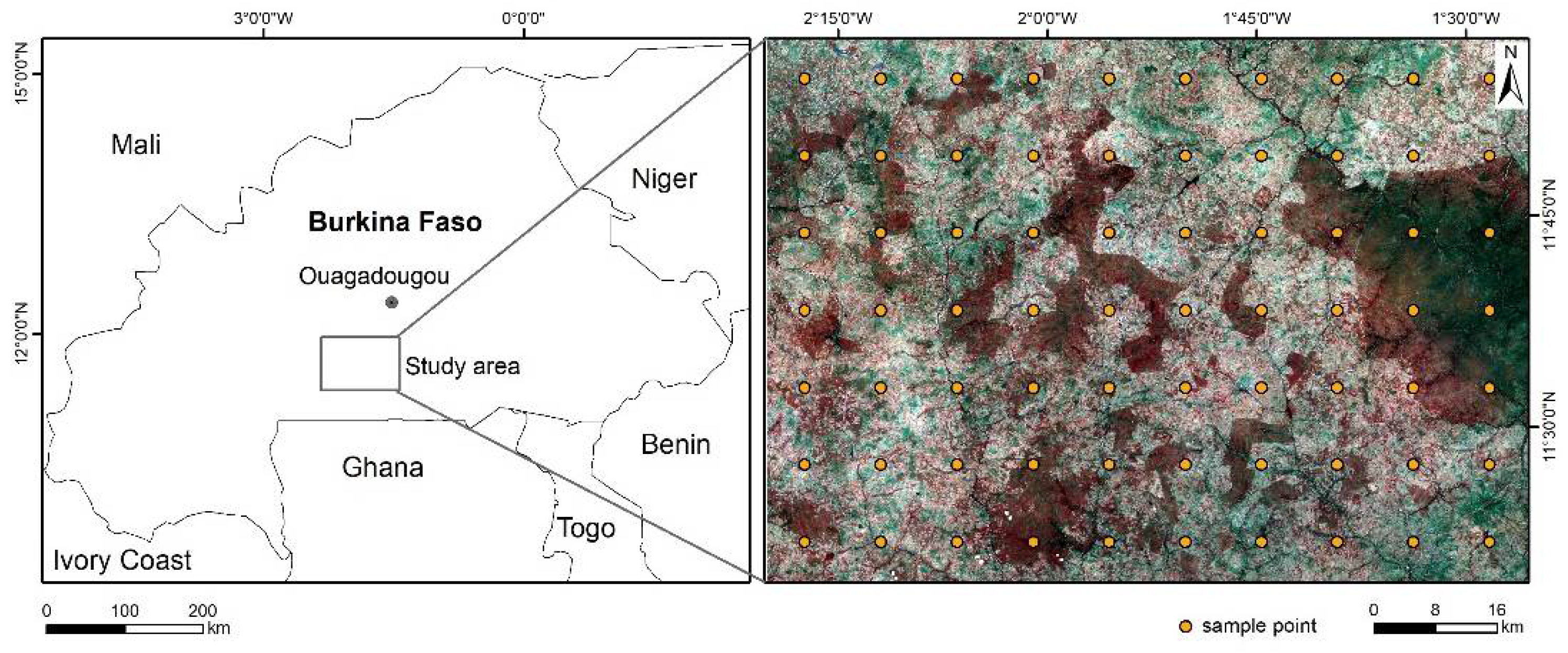
Our study area is located in southern Burkina Faso, belonging the West Sudanian savanna ecoregion (Figure 1). The mean annual precipitation was 827 mm, and the mean annual temperature was 27.5 °C [16]. Tropical dry forests and woodlands are surrounded by agroforestry parklands and agricultural fields. There was an increased conversion of forests and woodland into cropland during the last decade [17]. Fires, due to anthropogenic and natural reasons, occur regularly. Most of the fires take place during the dry season between November and February, even in early October, and late March and April. Burned vegetation typically recovers quickly without causing permanent land cover change.

Figure 1.
Study area and the distribution of random systematic sampling points based on Landsat 5 image acquired on 15 November 2014.
We collected all available Landsat Surface Reflectance data with WRS-2 coordinates Path 195 Row 52 from the Earth Resources Observations and Science (EROS) Center Archive for the time period between October 2000 and April 2016, which was the same data in Liu et al. [15] for burned area detection. The full time series used in the study consisted of 281 images, including 40 Landsat 5 Thematic Mapper (TM) images, 185 Landsat 7 Enhanced Thematic Mapper Plus (ETM+) images, and 56 Landsat 8 Operational Land Imager (OLI) images. Table 1 shows the number of Landsat images from October in one year to September in the next year ranging from 2000 to 2015. In 2015–2016, images were from October 2015 to April 2016. All images have been atmospherically corrected, and clouds and shadows have been removed using the Fmask algorithm [18]. We selected surface reflectance in blue, green, red, near-infrared (NIR), and two shortwave infrared (SWIR1, SWIR2) bands for further analysis.

Table 1.
Frequency of all available Landsat images for the study area by year.
2.2. Burned Area Detection Algorithm Using Landsat Time Series
The algorithm for detecting burned areas with different spectral indices included four steps. First, the BFAST Monitor (Breaks for Additive Season and Trend Monitor) algorithm [19] was applied to detect land cover change using Landsat NDVI time series. Next, a harmonic model was fitted using different spectral indices for each stable period without land cover change. Then the outliers caused by fire events were detected by comparing model predictions with the observed values using an optimal threshold for different spectral indices. The optimal threshold was determined separately based on the performance of burned area detection with different spectral indices. The burned area pixels were combined from every single image into an annual Landsat burned area within fire season. Finally, we performed accuracy assessments using reference data interpreted from Landsat images and compared the performance of different spectral indices in burned area detection. Fusion of different spectral indices burned area detection results was also tested.
2.2.1. Breakpoint Detection Using Landsat Time Series
We applied the BFAST Monitor approach to detect deforestation in this study area described in more detail in Liu et al. [15]. The Landsat time series was separated into a historical period which is used as a baseline, and a monitoring period. We defined the baseline period between October 2000 and October 2002 as it is stable and has a minimum of nine observations for each pixel. The method fits a harmonic model to each pixel NDVI time series in a baseline period using ordinary least squares (OLS). By comparing the discrepancy between model predictions and observations in the monitoring period with a moving sums of residuals (MOSUM) approach, the breakpoint was detected when the deviation from zero was beyond a 95% significance boundary. The change magnitude was calculated by taking the median of all the residuals within the monitoring period. The disturbance pixel was determined by a breakpoint pixel with negative magnitude [19]. Each pixel-wise time series had its own stable period after detecting land cover change. The pixels without land cover change were regarded as stable from 2000 to 2016, and the pixels with breakpoints were separated into before and after land cover change periods, respectively.
2.2.2. Spectral Indices for Burned Area Detection
Following previous burned area mapping studies, several spectral indices were included and tested in our study based on their performance (Table 2). NDVI is sensitive to vegetation greenness and is widely used in burned area mapping studies. The Soil Adjusted Vegetation Index (SAVI) is selected as it suppresses the influence of soil brightness and improves the separability of burns from soil and water. The Enhanced Vegetation Index (EVI) does not saturate as quickly in high biomass regions by minimizing the effects of soil and atmosphere. The Global Environmental Monitoring Index (GEMI) is designed to minimize the influence of atmospheric effects, which are considered very important for dark surface detection. We also included the indices specifically developed for burn detection because they are sensitive to charcoal and ash deposition, such as NBR, NBR2, the Burned Area Index (BAI), the Burned Area Index Modified with longer SWIR band (BAIML), the Burned Area Index Modified with short SWIR band (BAIMs), and the Char Soil Index (CSI).
Table 2.
Summary of spectral indices. , ,,, and corresponds to surface reflectance in blue, red, near-infrared, short shortwave infrared, and long shortwave infrared spectral bands, respectively.
Large parts of the study area were burned during the dry season from November to March, and seasonal fires affected the spectral reflectance and indices, influencing the harmonic model fit and parameters. Therefore, the burned area detection method utilized the time series harmonic model with different spectral indices. We fitted a first order harmonic model considering the phenology in this study area which was driven by unimodal precipitation pattern. The following model was fit for each pixel:
where yt is the dependent variable (spectral index), t is the independent variable (time as Julian date), T is the temporal frequency (365 days), a, b and c are the model parameters representing intercept, amplitude, and phase coefficients in the harmonic model, respectively, and et is the residual error. Parameters a, b and c are derived using ordinary least squares (OLS) linear regression for each pixel [19,30,31]. In addition to model coefficients, the root mean square error (RMSE) is also calculated.
The method was applied to different spectral indices time series within their stable period. The method consisted of three steps. First, we generated different spectral indices image stacks from the Landsat time series. Second, we fitted the time series harmonic model using the observations from different spectral indices within the stable period as the dependent variable. Third, a threshold was selected to detect burned pixels by comparing the observed and predicted values. We used the threshold to detect the burned pixels, because the clear observations, were always within the model predicted ranges (±threshold × RMSE) when the land cover was stable. By contrast, the burned pixels deviated from the ranges, and the threshold in our analysis was ranging from 0.5×RMSE to 3.5×RMSE depending on the selected spectral indices. We applied the process iteratively until all the burned pixels were detected. The burned pixels from separate images were combined into the annual Landsat burned area during fire season by checking the date from the MODIS burned area product (MCD45A1) as described in Liu et al. [15].
2.2.3. Optimal Threshold Selection and Accuracy Assessment
Different spectral indices had their own optimal threshold in detecting burned areas. To compare their performance, it is necessary to determine the optimal threshold for each spectral index. The basic idea of the optimal threshold approach is to select a threshold value from the training samples, assuming that the optimal threshold value leading to the maximum accuracy in extracting the burned area within the training samples is also optimal for the entire image. There were 70 points covering the whole study area based on systematic random sampling (Figure 1). The distances between the points in the west–east direction and the north–south direction were all 10 km. The starting point of the sampling was selected randomly. Therefore, we had 1120 points in total, considering the 16 years of observations. Reference data for burned area detection is difficult to acquire over a long period of time. Therefore, we visually interpreted each reference point using all the available observations in the Landsat time series for accuracy assessment, as it was demonstrated to be a practical method in previous studies [13]. We randomly selected 30% reference samples to determine the optimal threshold for each spectral index. We compared the overall accuracy and determined the optimal threshold when the highest overall accuracy occurred. After the optimal threshold was determined for each spectral index, the accuracy assessment was conducted using 70% of the reference samples for each spectral index with the corresponding optimal threshold.
2.2.4. Fusion of the Burned Area Results Based on Different Spectral Indices
To test the potential of the fusion of burned area detection results with different spectral indices, a majority vote rule was adopted. To be specific, the burned area detection results with different spectral indices were ranked based on the overall accuracy, and we selected the best 3, 5, 7, 9, and 11 burned area detection results corresponding to the spectral indices to complete the fusion process. In the fusion process, a pixel was determined as a burned pixel if the number of the burned pixel votes was greater than half of the votes, with the votes representing the pixel was burned according to one spectral index.
3. Results
3.1. Breakpoint Detection
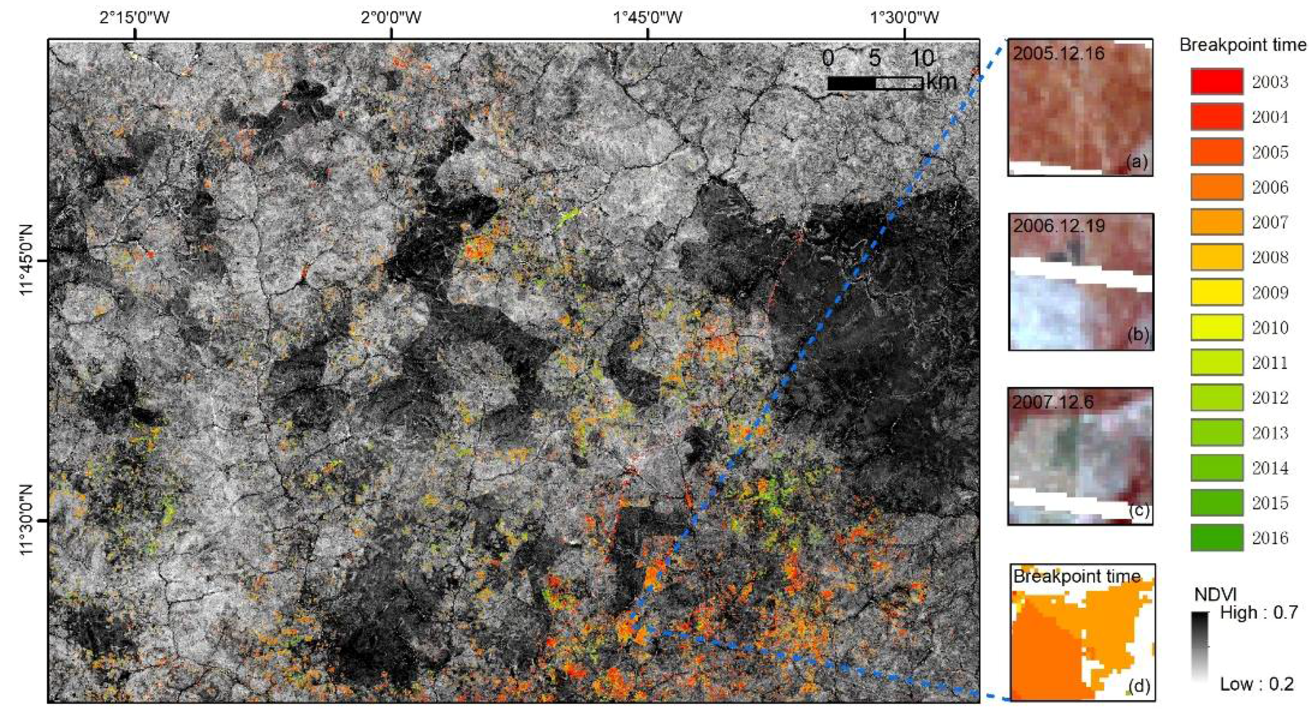
The disturbance map generated using the BFAST monitor method with Landsat time series is shown in Figure 2. Conversion from forest and woodlands to cropland was the main cause of the land cover change from 2003 to 2016 in this study area. We observed that most land cover changes occurred in the south-eastern part of the study area. The example showed in Figure 2 demonstrated that land cover change identified with breakpoint time.

Figure 2.
The disturbance map with breakpoint time (left panel), and an example of land cover change were identified (a,b,c,d) in the 2005–2007 period.
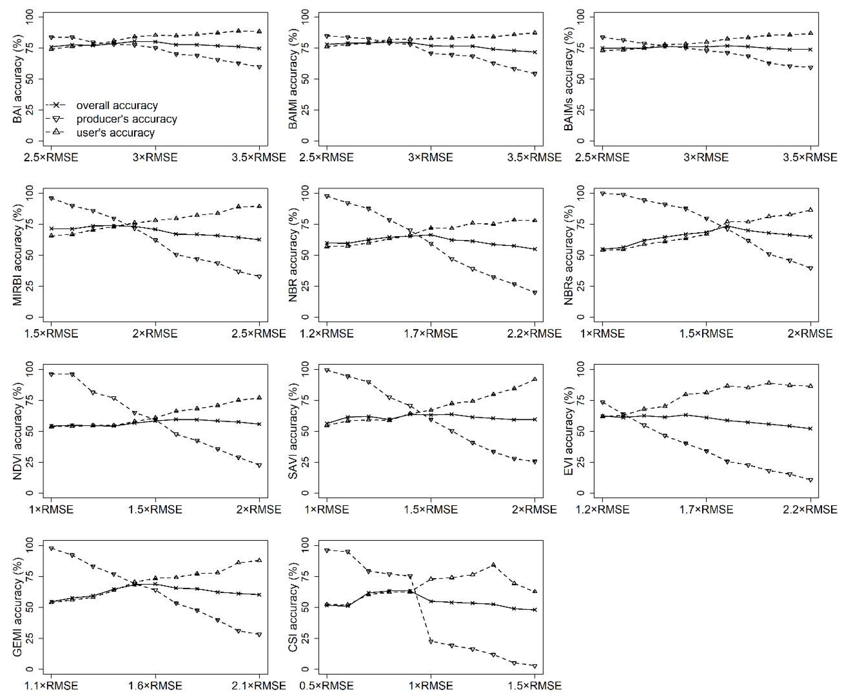
3.2. Optimal Threshold for Different Spectral Indices
The overall accuracy, producer’s accuracy, and user’s accuracy of burned area detection are demonstrated for a range of thresholds with different spectral indices (Figure 3). With an increasing threshold, the producer’s accuracy showed a decreasing trend, while in contrast, the user’s accuracy showed an increasing trend. The overall accuracy increased as the threshold increased, and then reached the peak value, but decreased as the threshold increased further. The optimal threshold is corresponding to the highest overall accuracy. Among all the tested indices, BAI achieved the best overall accuracy of 80.35% with a threshold of 2.9, followed by BAIML and BAIMs with thresholds of 2.8 and 3.1, respectively. NBR2 and MIRBI obtained overall accuracies around 73% and thresholds between 1.6 and 1.8. GEMI, NBR, SAVI, EVI, and NDVI had thresholds between 1.4 and 1.7. CSI provided an overall accuracy of 63.10% with a threshold of 0.8.
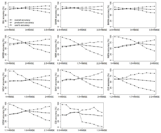
Figure 3.
Overall accuracy and producer’s and user’s accuracies for different spectral indices as a function of threshold value.
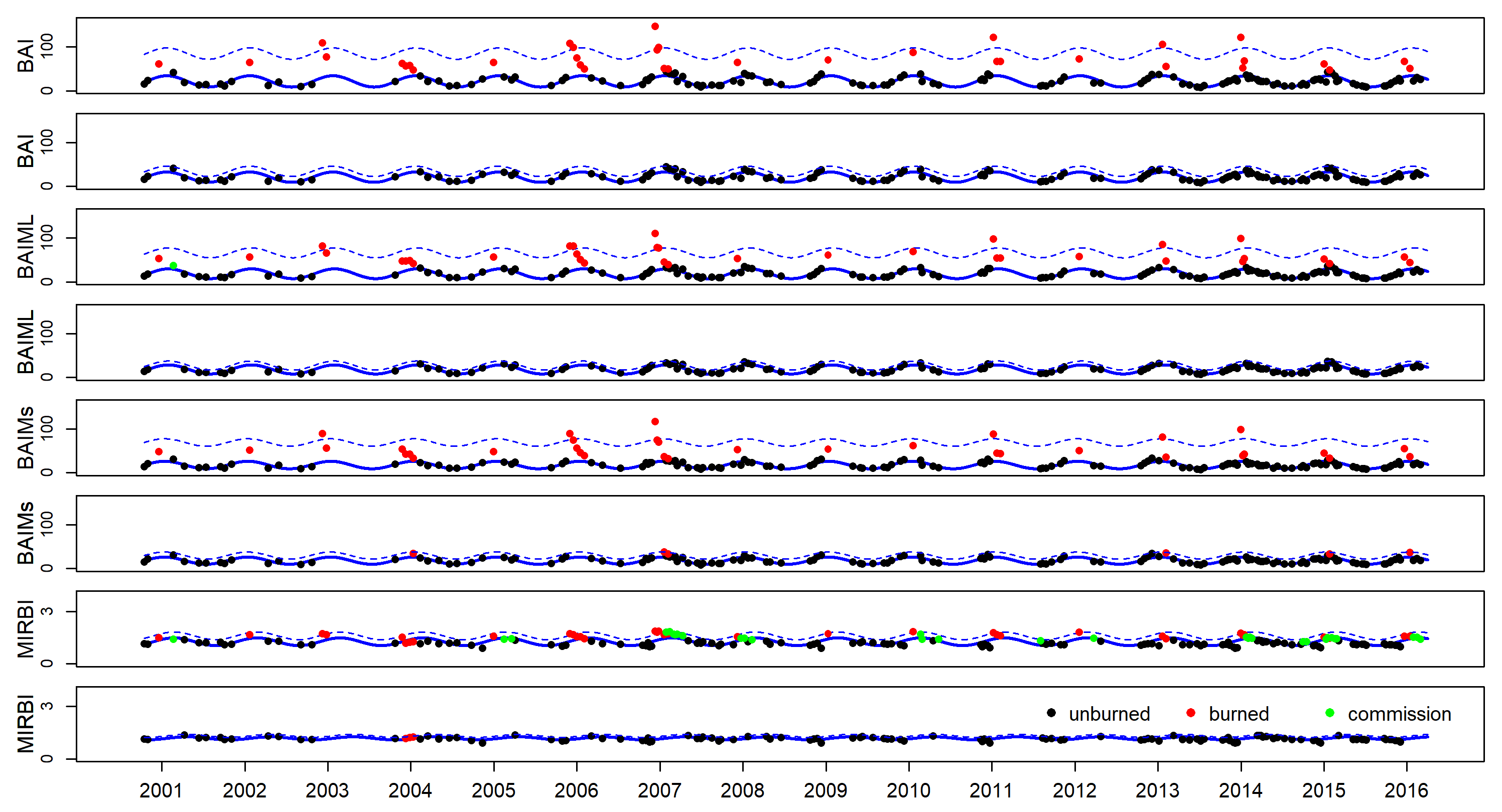
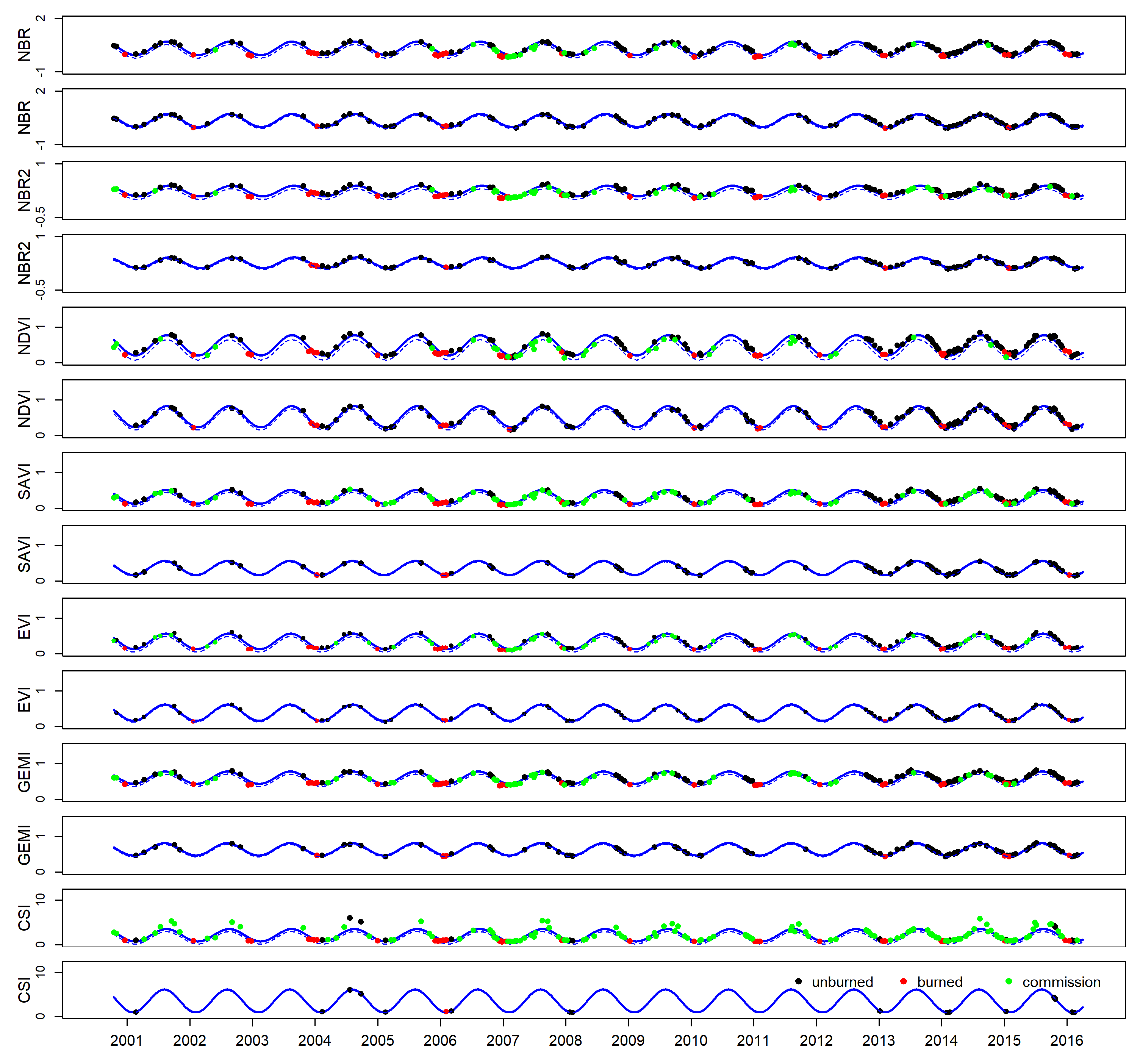
3.3. Pixel-Wise Time Series for Burned Area Detection Using Different Spectral Indices
Figure 4 and Figure 5 demonstrate the fit of the harmonic model before and after burned area detection for the same stable pixel time series with different spectral indices using an optimal threshold. Overall, the characteristics of burned pixels in the time series varied among different spectral indices time series. For BAI, BAIMs, BAIML, and MIRBI, the burned pixels had higher values compared to unburned pixels, by contrast, the burned pixels had lower values when compared to unburned pixels for NBR, NBR2, NDVI, SAVI, EVI, GEMI, and CSI. BAI time series achieved the best results by accurately detecting all the burned pixels, suggesting its sensitivity to burned signal. BAIMs and BAIML successfully captured most of the burned area in the time series with small omission and commission errors. More commission and omission errors were observed when using MIRBI, because there was only a subtle difference between burned and unburned values.
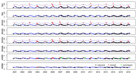
Figure 4.
Demonstration of harmonic model fit before and after burned area detection for a single pixel, based on different spectral indices with burned pixels having higher values than unburned pixels. The black points are unburned pixels, the red points are burned pixels, the green points are commission pixels, the blue curve is the harmonic model, and the dashed blue line is the threshold for detecting burned pixels.
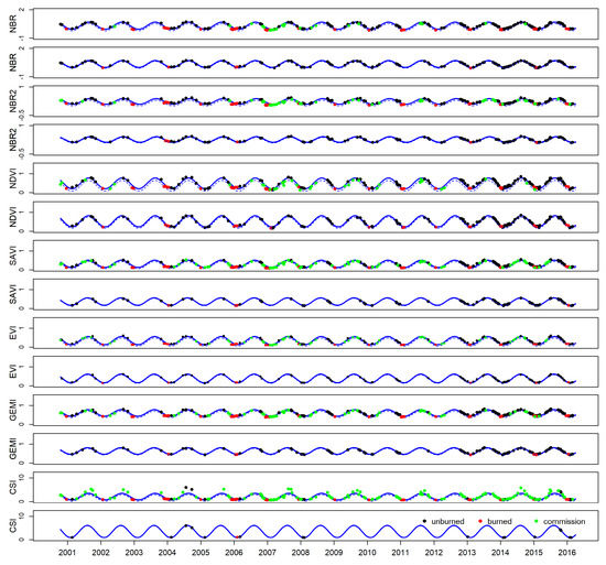
Figure 5.
Demonstration of harmonic model fit before and after burned area detection for a single pixel, based on different spectral indices with burned pixels having lower values than unburned pixels. The black points are unburned pixels, the red points are burned pixels, the green points are commission pixels, the blue curve is the harmonic model, and the dashed blue line is the threshold for detecting burned pixels.
The NBR, NBR2, NDVI, SAVI, EVI, and GEMI time series behaved similarly and revealed poor performances with more commission and omission errors, demonstrating the burned observations in these time series data could not be correctly distinguished from unburned observations. In CSI time series, unburned pixels showed more fluctuations, leading to the most commission errors among all the indices.
3.4. Burned Area Detection Comparison and Accuracy Assessment
We evaluated the overall accuracy, producer’s accuracy, and user’s accuracy of burned area detection for each spectral index with the optimal threshold (Table 3). The overall accuracies of burned area detection varied by different spectral indices. Among the spectral indices tested, the most accurate was the BAI, with a good balance of commission and omission errors (overall accuracy 77.81%). The next best accuracies were achieved by BAIMs, BAIML, and MIRBI with similar performance (72.45% to 76.40%). NBR2 and NBR achieved overall accuracies of 70.79% and 66.71%, respectively. The overall accuracies for greenness-related spectral indices (GEMI, EVI, SAVI, NDVI) was between 63.52% and 67.99%, while GEMI outperformed EVI, SAVI, and NDVI, being the best vegetation index for burned area mapping among the four vegetation indices. The least successful spectral index was CSI, with an overall accuracy of 56.89%.
Table 3.
Accuracy assessment for different classifications.
The performance of fusion of different spectral indices with the majority vote method depended on the number of spectral indices used. In the fusion process, the overall accuracies increased as the number of spectral indices increased from 3 to 9, but decreased as the number of spectral indices increased further to 11. The best combination of spectral indices achieved an overall accuracy of 78.57% with a fusion of 7 or 9 spectral indices, with a slight increase compared to the best single spectral index BAI.
4. Discussion
Spectral indices are widely utilized in burned area monitoring, and different spectral indices are used in various environments to improve burned area detection accuracy. In this study, we tested different spectral indices in burned area detection over a savanna environment with Landsat time series.
We found that the most accurate spectral index tested in our study was BAI, followed by BAIMs and BAIML. This result was in line with previous studies demonstrating that BAI is effective in burned area detection, including the savanna environment [32]. Several studies confirm the potential of BAI in discriminating burned areas from other land cover types, due to its higher sensitivity to char signal in post-fire images in comparison to other spectral indices. MIRBI achieved a moderate accuracy among all the spectral indices, and it was found to discriminate burned area from soil and arable land, but not from shadows [33]. Our results also indicated that NBR and NBR2 are unsuitable for accurate burned area estimations, even though NBR is a common spectral index and widely applied in burned severity assessment [1]. The main reason is that NBR is more suitable for burned area detection for a short time after the fire, and hence, its use is limited by the temporal resolution of Landsat data [34]. Further assessments are necessary to evaluate the influence of the Landsat temporal resolution on the capability to detect and measure vegetation recovery, as well as how higher temporal resolution sensors would improve the detection of vegetation recovery dynamics after fire events. In addition, NBR has been proved to be less sensitive to burned areas in savanna environments, because of the general decrease in reflectance in all spectral bands in response to fire [13].
The vegetation indices, NDVI, SAVI, EVI, and GEMI, performed similarly, with limited capacity to identify a fire-affected area with other studies confirming these findings [11]. The main reason is that they were designed to determine vegetation properties, not intended for burned area detection. The low accuracies are mainly caused by confusions between the burned area with dark surfaces, such as soil, shadow, and water, and especially in the dry season, the characteristic of the vegetation can lead to errors and confusion with burned areas [20]. CSI was the least successful in burned area estimation among all the spectral indices, and our findings on the poor performance of CSI in burned area detection are similar to those by Schepers et al. [35], who pointed that CSI easily confused char signal with soil.
The performance of burned area detection using a fusion of different spectral indices depended on the number of selected spectral indices, suggesting careful selection is necessary when fusing burned areas detection based on several spectral indices. However, the small improvement in the overall accuracy in comparison to the best index (BAI) suggests that there are only minor complementary benefits among the best indices in the studied environment, although greater benefits might be attained elsewhere. Considering that selecting the best indices for fusion can vary from one region to another, burned area detection based on BAI remains a logical first choice for burned area monitoring. However, the method based on fuzzy set theory could be a more effective way to combine indices as indicated by a previous study [36]; hence, it deserves to be tested in future studies.
5. Conclusions
In this study, we explored the performance and sensitivity of eleven different spectral indices on burned area detection with Landsat time series in the savanna area of southern Burkina Faso. The burned area detection method was based on breakpoint identification and harmonic model fitting with Landsat data from 2000 to 2016. The result demonstrated that BAI was the most accurate index for burned area mapping among all the tested spectral indices. Fire-related spectral indices outperformed vegetation indices, and CSI performed worst in burned area detection. Fusing different spectral indices only achieved minor improvement in accuracy in our study area, and the number of selected spectral indices influenced the burned area mapping performance.
Author Contributions
Conceptualization, J.L., J.H.; methodology, J.L., E.E.M. and J.H.; software, J.L. and D.W.; validation, J.L.; formal analysis, J.L.; investigation, J.L., E.E.M. and J.H.; resources, J.L., E.E.M. and J.H.; data curation, J.L., E.E.M. and J.H.; writing—original draft preparation, J.L. and D.W.; writing—review and editing, J.L., D.W., E.E.M. and J.H.; visualization, J.L. and D.W.; supervision, E.E.M. and J.H. All authors have read and agreed to the published version of the manuscript.
Funding
This research was supported by the Fundamental Research Funds for the Central Universities (grant number 2652018077), Building Bio-Carbon and Rural Development in West Africa (BIODEV) program funded by the Ministry for Foreign Affairs of Finland, and Academy of Finland (decision numbers 318252 and 319905).
Data Availability Statement
The Landsat data is downloaded from Earth Explorer (http://earthexplorer.usgs.gov/ accessed on 17 May 2021). MODIS burned area product (MCD45A1) is downloaded from http://modis-fire.umd.edu/ (accessed on 17 May 2021).
Acknowledgments
The authors are grateful to the editors and the anonymous reviewers for their suggestions for improving the manuscript. We also thank some data agencies who contributed to the datasets used in this study.
Conflicts of Interest
The authors declare no conflict of interest.
References
- Musyimi, Z.; Said, M.Y.; Zida, D.; Rosenstock, T.S.; Udelhoven, T.; Savadogo, P.; de Leeuw, J.; Aynekulu, E. Evaluating Fire Severity in Sudanian Ecosystems of Burkina Faso Using Landsat 8 Satellite Images. J. Arid. Environ. 2017, 139, 95–109. [Google Scholar] [CrossRef]
- Siljander, M. Predictive Fire Occurrence Modelling to Improve Burned Area Estimation at a Regional Scale: A Case Study in East Caprivi, Namibia. Int. J. Appl. Earth Obs. Geoinf. 2009, 11, 380–393. [Google Scholar] [CrossRef]
- Mouillot, F.; Schultz, M.G.; Yue, C.; Cadule, P.; Tansey, K.; Ciais, P.; Chuvieco, E. Ten Years of Global Burned Area Products from Spaceborne Remote Sensing-A Review: Analysis of User Needs and Recommendations for Future Developments. Int. J. Appl. Earth Obs. Geoinf. 2014, 26, 64–79. [Google Scholar] [CrossRef] [Green Version]
- Koutsias, N.; Pleniou, M.; Mallinis, G.; Nioti, F.; Sifakis, N.I. A Rule-Based Semi-Automatic Method to Map Burned Areas: Exploring the USGS Historical Landsat Archives to Reconstruct Recent Fire History. Int. J. Remote Sens. 2013, 34, 7049–7068. [Google Scholar] [CrossRef]
- Kontoes, C.C.; Poilve, H.; Florsch, G.; Keramitsoglou, I.; Paralikidis, S. A Comparative Analysis of a Fixed Thresholding vs. a Classification Tree Approach for Operational Burn Scar Detection and Mapping. Int. J. Appl. Earth Obs. Geoinf. 2009, 11, 299–316. [Google Scholar] [CrossRef]
- Maeda, E.E.; Formaggio, A.R.; Shimabukuro, Y.E.; Balue Arcoverde, G.F.; Hansen, M.C. Predicting Forest Fire in the Brazilian Amazon Using MODIS Imagery and Artificial Neural Networks. Int. J. Appl. Earth Obs. Geoinf. 2009, 11, 265–272. [Google Scholar] [CrossRef]
- Koutsias, N.; Mallinis, G.; Karteris, M. A Forward/Backward Principal Component Analysis of Landsat-7 ETM+ Data to Enhance the Spectral Signal of Burnt Surfaces. ISPRS-J. Photogramm. Remote Sens. 2009, 64, 37–46. [Google Scholar] [CrossRef]
- Hardtke, L.A.; Blanco, P.D.; del Valle, H.F.; Metternicht, G.I.; Sione, W.F. Semi-Automated Mapping of Burned Areas in Semi-Arid Ecosystems Using MODIS Time-Series Imagery. Int. J. Appl. Earth Obs. Geoinf. 2015, 38, 25–35. [Google Scholar] [CrossRef]
- Smith, A.M.S.; Drake, N.A.; Wooster, M.J.; Hudak, A.T.; Holden, Z.A.; Gibbons, C.J. Production of Landsat ETM plus Reference Imagery of Burned Areas within Southern African Savannahs: Comparison of Methods and Application to MODIS. Int. J. Remote Sens. 2007, 28, 2753–2775. [Google Scholar] [CrossRef]
- Veraverbeke, S.; Harris, S.; Hook, S. Evaluating Spectral Indices for Burned Area Discrimination Using MODIS/ASTER (MASTER) Airborne Simulator Data. Remote Sens. Environ. 2011, 115, 2702–2709. [Google Scholar] [CrossRef]
- Stroppiana, D.; Boschetti, M.; Zaffaroni, P.; Brivio, P.A. Analysis and Interpretation of Spectral Indices for Soft Multicriteria Burned-Area Mapping in Mediterranean Regions. IEEE Geosci. Remote Sens. Lett. 2009, 6, 499–503. [Google Scholar] [CrossRef]
- Liu, S.; Zheng, Y.; Dalponte, M.; Tong, X. A Novel Fire Index-Based Burned Area Change Detection Approach Using Landsat-8 OLI Data. Eur. J. Remote Sens. 2020, 53, 104–112. [Google Scholar] [CrossRef] [Green Version]
- Goodwin, N.R.; Collett, L.J. Development of an Automated Method for Mapping Fire History Captured in Landsat TM and ETM plus Time Series across Queensland, Australia. Remote Sens. Environ. 2014, 148, 206–221. [Google Scholar] [CrossRef]
- Hawbaker, T.J.; Vanderhoof, M.K.; Beal, Y.-J.; Takacs, J.D.; Schmidt, G.L.; Falgout, J.T.; Williams, B.; Fairaux, N.M.; Caldwell, M.K.; Picotte, J.J.; et al. Mapping Burned Areas Using Dense Time-Series of Landsat Data. Remote Sens. Environ. 2017, 198, 504–522. [Google Scholar] [CrossRef]
- Liu, J.; Heiskanen, J.; Maeda, E.E.; Pellikka, P.K.E. Burned Area Detection Based on Landsat Time Series in Savannas of Southern Burkina Faso. Int. J. Appl. Earth Obs. Geoinf. 2018, 64, 210–220. [Google Scholar] [CrossRef] [Green Version]
- Hijmans, R.J.; Cameron, S.E.; Parra, J.L.; Jones, P.G.; Jarvis, A. Very High Resolution Interpolated Climate Surfaces for Global Land Areas. Int. J. Climatol. 2005, 25, 1965–1978. [Google Scholar] [CrossRef]
- Gessner, U.; Knauer, K.; Kuenzer, C.; Dech, S. Land Surface Phenology in a West African Savanna: Impact of Land Use, Land Cover and Fire. In Remote Sensing Time Series; Kuenzer, C., Dech, S., Wagner, W., Eds.; Remote Sensing and Digital Image Processing; Springer International Publishing: Dordrecht, The Netherlands, 2015; Volume 22, pp. 203–223. ISBN 978-3-319-15967-6. [Google Scholar]
- Zhu, Z.; Woodcock, C.E. Object-Based Cloud and Cloud Shadow Detection in Landsat Imagery. Remote Sens. Environ. 2012, 118, 83–94. [Google Scholar] [CrossRef]
- DeVries, B.; Verbesselt, J.; Kooistra, L.; Herold, M. Robust Monitoring of Small-Scale Forest Disturbances in a Tropical Montane Forest Using Landsat Time Series. Remote Sens. Environ. 2015, 161, 107–121. [Google Scholar] [CrossRef]
- Chuvieco, E.; Martin, M.P.; Palacios, A. Assessment of Different Spectral Indices in the Red-near-Infrared Spectral Domain for Burned Land Discrimination. Int. J. Remote Sens. 2002, 23, 5103–5110. [Google Scholar] [CrossRef]
- Martín, M.P.; Gómez, I.; Chuvieco, E. Burnt Area Index (BAIM) for Burned Area Discrimination at Regional Scale Using MODIS Data. For. Ecol. Manag. 2006, 234, S221. [Google Scholar] [CrossRef]
- Trigg, S.; Flasse, S. An Evaluation of Different Bi-Spectral Spaces for Discriminating Burned Shrub-Savannah. Int. J. Remote Sens. 2001, 22, 2641–2647. [Google Scholar] [CrossRef]
- Smith, A.M.S.; Wooster, M.J.; Drake, N.A.; Dipotso, F.M.; Falkowski, M.J.; Hudak, A.T. Testing the Potential of Multi-Spectral Remote Sensing for Retrospectively Estimating Fire Severity in African Savannahs. Remote Sens. Environ. 2005, 97, 92–115. [Google Scholar] [CrossRef] [Green Version]
- Tucker, C.J. Red and Photographic Infrared Linear Combinations for Monitoring Vegetation. Remote Sens. Environ. 1979, 8, 127–150. [Google Scholar] [CrossRef] [Green Version]
- Key, C.H.; Benson, N.C. The Normalized Burn Ratio (NBR): A Landsat TM Radiometric Measure of Burn Severity; United States Geological Survey, Northern Rocky Mountain Science Center: Bozeman, MT, USA, 1999. [Google Scholar]
- Lutes, D.C.; Keane, R.E.; Caratti, J.F.; Key, C.H.; Benson, N.C.; Sutherland, S.; Gangi, L.J. FIREMON: Fire Effects Monitoring and Inventory System; US Department of Agriculture, Forest Service, Rocky Mountain Research Station: Fort Collins, CO, USA, 2006; Gen. Tech. Rep. RMRS-GTR-164. 1 CD. [Google Scholar]
- Pinty, B.; Verstraete, M. Gemi—a Nonlinear Index to Monitor Global Vegetation from Satellites. Vegetatio 1992, 101, 15–20. [Google Scholar] [CrossRef]
- Huete, A. A Soil-Adjusted Vegetation Index (Savi). Remote Sens. Environ. 1988, 25, 295–309. [Google Scholar] [CrossRef]
- Huete, A.; Didan, K.; Miura, T.; Rodriguez, E.P.; Gao, X.; Ferreira, L.G. Overview of the Radiometric and Biophysical Performance of the MODIS Vegetation Indices. Remote Sens. Environ. 2002, 83, 195–213. [Google Scholar] [CrossRef]
- Verbesselt, J.; Zeileis, A.; Herold, M. Near Real-Time Disturbance Detection Using Satellite Image Time Series. Remote Sens. Environ. 2012, 123, 98–108. [Google Scholar] [CrossRef]
- Zhu, Z.; Woodcock, C.E. Continuous Change Detection and Classification of Land Cover Using All Available Landsat Data. Remote Sens. Environ. 2014, 144, 152–171. [Google Scholar] [CrossRef] [Green Version]
- Disney, M.I.; Lewis, P.; Gomez-Dans, J.; Roy, D.; Wooster, M.J.; Lajas, D. 3D Radiative Transfer Modelling of Fire Impacts on a Two-Layer Savanna System. Remote Sens. Environ. 2011, 115, 1866–1881. [Google Scholar] [CrossRef]
- Bastarrika, A.; Chuvieco, E.; Pilar Martin, M. Mapping Burned Areas from Landsat TM/ETM plus Data with a Two-Phase Algorithm: Balancing Omission and Commission Errors. Remote Sens. Environ. 2011, 115, 1003–1012. [Google Scholar] [CrossRef]
- Fornacca, D.; Ren, G.; Xiao, W. Evaluating the Best Spectral Indices for the Detection of Burn Scars at Several Post-Fire Dates in a Mountainous Region of Northwest Yunnan, China. Remote Sens. 2018, 10, 1196. [Google Scholar] [CrossRef] [Green Version]
- Schepers, L.; Haest, B.; Veraverbeke, S.; Spanhove, T.; Vanden Borre, J.; Goossens, R. Burned Area Detection and Burn Severity Assessment of a Heathland Fire in Belgium Using Airborne Imaging Spectroscopy (APEX). Remote Sens. 2014, 6, 1803–1826. [Google Scholar] [CrossRef] [Green Version]
- Stroppiana, D.; Bordogna, G.; Boschetti, M.; Carrara, P.; Boschetti, L.; Brivio, P.A. Positive and Negative Information for Assessing and Revising Scores of Burn Evidence. IEEE Geosci. Remote Sens. Lett. 2012, 9, 363–367. [Google Scholar] [CrossRef]
Publisher’s Note: MDPI stays neutral with regard to jurisdictional claims in published maps and institutional affiliations. |
© 2021 by the authors. Licensee MDPI, Basel, Switzerland. This article is an open access article distributed under the terms and conditions of the Creative Commons Attribution (CC BY) license (https://creativecommons.org/licenses/by/4.0/).