Article

Combining Multiple Geospatial Data for Estimating Aboveground Biomass in North Carolina Forests

by
Leila Hashemi-Beni
1,*,†,
Lyubov A. Kurkalova
2,†,
Timothy J. Mulrooney
3 and
Chinazor S. Azubike
4
1
Geomatics Program, Department of Built Environment, North Carolina A&T State University, Greensboro, NC 27411, USA
2
Department of Economics, North Carolina A&T State University, Greensboro, NC 27411, USA
3
Department of Environmental, Earth and Geospatial Sciences, North Carolina Central University, Durham, NC 27707, USA
4
Applied Science and Technology Program, North Carolina A&T State University, Greensboro, NC 27411, USA
*
Author to whom correspondence should be addressed.
Leila Hashemi-Beni and Lyubov A. Kurkalova two authors share the same contribution to this article.
Remote Sens. 2021, 13(14), 2731; https://doi.org/10.3390/rs13142731
Submission received: 10 June 2021 / Revised: 2 July 2021 / Accepted: 6 July 2021 / Published: 12 July 2021
(This article belongs to the Section Forest Remote Sensing)

Abstract

:
Mapping and quantifying forest inventories are critical for the management and development of forests for natural resource conservation and for the evaluation of the aboveground forest biomass (AGFB) technically available for bioenergy production. The AGFB estimation procedures that rely on traditional, spatially sparse field inventory samples constitute a problem for geographically diverse regions such as the state of North Carolina in the southeastern U.S. We propose an alternative AGFB estimation procedure that combines multiple geospatial data. The procedure uses land cover maps to allocate forested land areas to alternative forest types; uses the light detection and ranging (LiDAR) data to evaluate tree heights; calculates the area-total AGFB using region- and tree-type-specific functions that relate the tree heights to the AGFB. We demonstrate the procedure for a selected North Carolina region, a 2.3 km2 area randomly chosen in Duplin County. The tree diameter functions are statistically estimated based on the Forest Inventory Analysis (FIA) data, and two publicly available, open source land cover maps, Crop Data Layer (CDL) and National Land Cover Database (NLCD), are compared and contrasted as a source of information on the location and typology of forests in the study area. The assessment of the consistency of forestland mapping derived from the CDL and the NLCD data lets us estimate how the disagreement between the two alternative, widely used maps affects the AGFB estimation. The methodology and the results we present are expected to complement and inform large-scale assessments of woody biomass in the region.

Graphical Abstract

1. Introduction

The mapping and quantifying of forest inventory dynamics are critical for the management and development of forests for natural resource conservation [1,2] as well as for the evaluation of the aboveground forest biomass (AGFB) technically available for bioenergy production [3,4]. Understanding the inventories is also important for the economic assessment of forests as a source of material for wood products. Two major wood products that could be economically competitive for different geographic regions are saw timber and pulp. Forests in the southeastern U.S. have recently attracted additional attention because of the growth in wood pellet production, and the leading role of the region in the world wood-pellet production capacity [3,5,6,7,8].
Existing assessments of southeastern U.S. forest growth and removal have mostly been based on U.S. Department of Agriculture Forest Service Forest Inventory and Analysis (FIA) surveys [3,6,7,9,10,11,12,13]. The FIA data are collected on a stratified sample of forestland plots, usually in 5–7 year intervals in the southeastern U.S. [14,15], and the nationally standardized database provides a consistent framework for developing and storing forest inventory data across all ownerships for the entire country [16].
Exclusive reliance on the FIA dataset has limitations in assessing forest inventories for relatively small geographic areas, where the traditional field inventory methods constitute a problem for geographically diverse regions such as North Carolina. The state is one of the most physio-geographically diverse states in the southern U.S. [14], and the diversity of the state’s geography contributes to significant variability in forest types and density (NCFS, 2017). However, each North Carolina sample point represents, on average, over 1200 hectares [10]. The relatively sparse sample of FIA is the reason why the database is not recommended for evaluating forest inventories on smaller geographic scales, such as counties or smaller.
Recognizing the need for understanding the spatial distribution of the forest biomass at a fine spatial resolution (e.g., at a 30 m resolution), multiple studies of the AGFB led to using remote sensing methods for the data obtained. Two groups of such data stand out when it comes to the evaluation of the AGFB for contiguous regions: three-dimensional measurements obtained with light detection and ranging (LiDAR) technology and vegetation maps derived from satellite imagery or aerial photography [17,18,19].
LiDAR is a high-resolution active remote sensing technology that uses light in the form of a pulsed laser to densely sample the earth’s surface. The LiDAR data can be used to calculate the density and the height of vegetation across areas, and have been used to extensively estimate the AGFB [19,20,21]. However, LiDAR coverage could be of limited availability, is usually costly, may be proprietary, and could be challenging for temporal resolutions of interest [19,22] and for differentiating between forests of alternative types [21]. To compensate for these potential deficiencies, some studies integrated LiDAR measurements with ground observations, such as those from the FIA [1,23,24].
Digital maps resulting from the analysis of remotely sensed data allow for the characterization of land cover for large geographic areas and could be relatively inexpensive to develop. However, for the purposes of AGFB evaluation, the maps need to be combined with auxiliary data to evaluate the height and the density of the forests. A few studies integrated ground observations with vegetation maps for the evaluation of the AGFB. The U.S. applications of such an approach have been reported for Wisconsin [17], Minnesota [25], and the Utah High Plateaus [18]. We propose a different data integration approach, the one that combines LiDAR with digital maps.
In the U.S., two major sources of remote sensing-based cover data are Crop Data Layer (CDL) [26] and the National Land Cover Database (NLCD) [27]. The NLCD provides comprehensive, spatially explicit, national U.S. land cover description in approximately five-year intervals [27]. The data, developed by a group of U.S. federal agencies, is represented by a 16-class land cover classification scheme at a spatial resolution of 30 m. Recent NLCD collections (2001, 2006, 2011, and 2016) have maintained a consistent land cover classification scheme, including water, developed land, barren, forest, shrubland, herbaceous, planted/cultivated land, and wetlands, at a spatial resolution of 30 m.
CDL is an annual, raster, geo-referenced, crop-specific land cover data layer developed by the National Agricultural Statistics Service of the U.S. Department of Agriculture [26], with the same spatial resolution of 30 m. While the focus of the data is on cropland, the information on several non-cropland categories is also collected. Similar to the NLCD, CDL forest land cover categories include deciduous forest, evergreen forest, mixed forest, and woody wetlands. Although the CDL is updated every year, only a few studies assessed the usefulness of the CDL for forest assessment [17,28], likely because the dataset is relatively new: the CDL provides complete coverage of all of the U.S. states since 2008 only. While both the NLCD and CDL are effective for mapping forest land, these sources alone are insufficient for the assessment of the AGFB, because the amount of biomass also depends on the height and diameter of the trees.
This study proposes a new approach to the estimation of the AGFB that combines the land use information easily available in land use maps with LiDAR data. Our demonstration of the approach highlights the impact of the potential errors present in alternative, widely-available land use data sources, CDL and the NLCD, on the resulting AGFB estimates. For a selected region of the state, a 2.3 km2 area randomly chosen in Duplin County, we assess the consistency of forestland mapping derived from CDL and the NLCD; overlay the maps derived from both CDL and the NLCD with LiDAR data to derive tree canopy surface and evaluate tree heights; use the FIA data to statistically estimate functions that relate tree heights to tree diameters and to derive the tree height to the AGFB functions, by forest type; estimate the study-area-total AGFB, while explicitly assessing how the disagreement between the NLCD and CDL affects the estimates. The methodology and the results we present are expected to complement and inform large-scale assessments of woody biomass in the region.

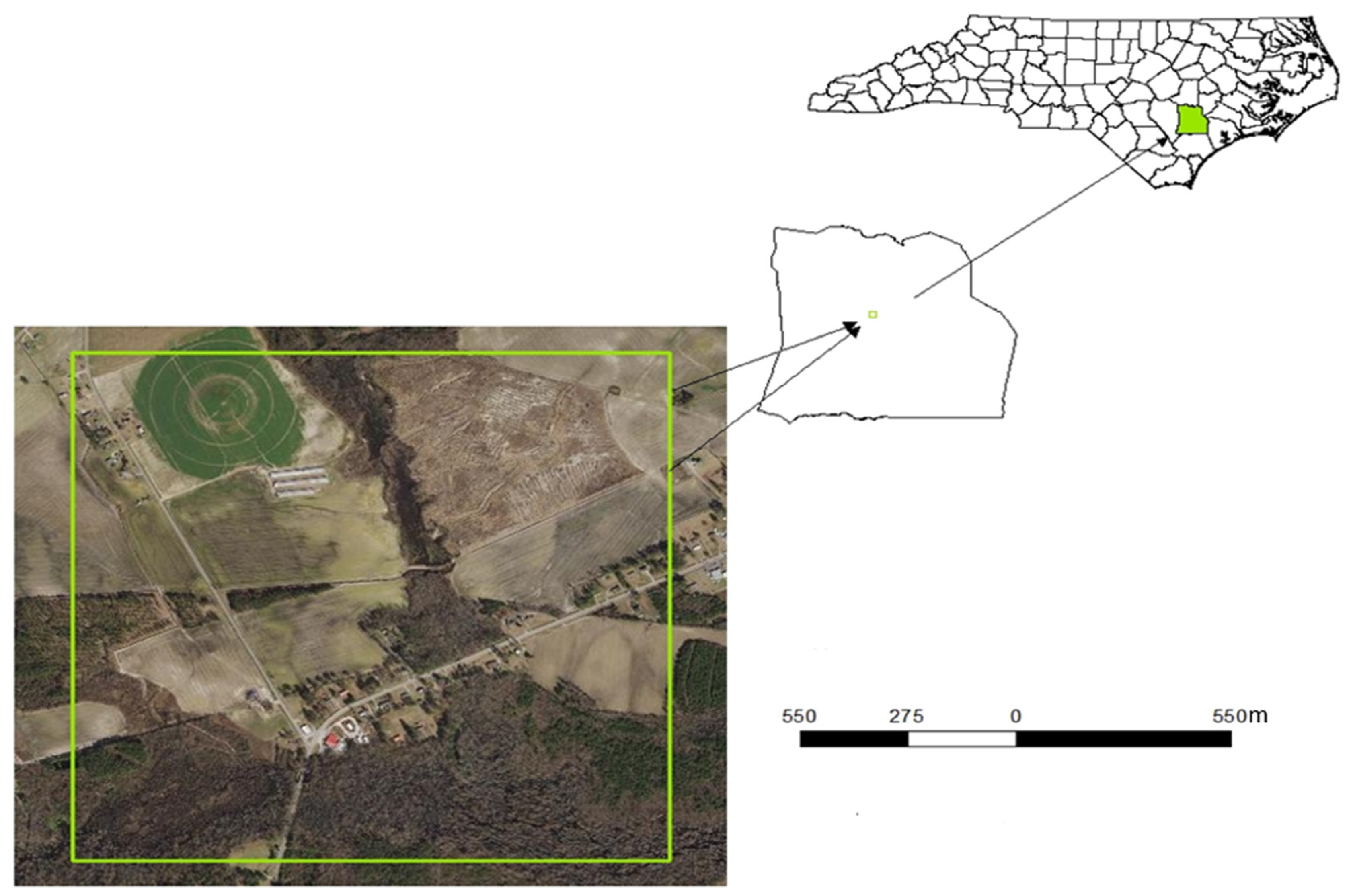
2. Data and Study Area

According to the latest available North Carolina FIA inventory cycle completed in 2013, forests occupied approximately 60% of the state’s land between 2007 and 2013 [14]. FIA surveys divide the state into four regions (units), with the percent of area forested varying between 51% in the central, Piedmont unit, and 76% in the western, Mountains unit. The total forested area in the Southern Coastal Plain unit is the closest to the state average; it remained stable at 61% between 1999 and 2013 [14]. For the purpose of the presentation of the AGFB estimation procedure, we randomly selected a 2.3 km2 study area in that unit. The area is located in Duplin County (Figure 1).
The four datasets used in this study are 2011 NCDL, 2011 NLCD, 2013 high-resolution LIDAR, and 2009–2013 FIA:
(a)
The NLCD for the year 2011 was downloaded from the MLRC, 2021 [27]. While the 2016 version of the NLCD is the latest available, it is outside of the range covered by the latest FIA data available for the state;
(b)
CDL for the year 2011 was downloaded from the USDA, 2021 [26]. We chose the 2011 CDL data to allow for the comparison of CDL and the NLCD in the same year;
(c)
LiDAR data for the year 2013 was downloaded from the North Carolina Geospatial website (https://sdd.nc.gov/, accessed on 1 June 1 2021);
(d)
FIA for 2009–2013 were downloaded from (https://apps.fs.usda.gov/fia/datamart/CSV/datamart_csv.html, accessed on 1 June 2021). The data comes from the latest completed North Carolina FIA inventory cycle.

3. Methods

Following convention, we define AGFB as the oven-dry mass of the aboveground portion of a tree, which includes stem wood, stump, bark, top, branches, and foliage [15]. The AGFB estimation procedure we developed and implemented integrates land cover analysis, tree height estimation, and the estimation of region- and forest-type-specific tree diameter functions. The processes involved are summarized in Figure 2.

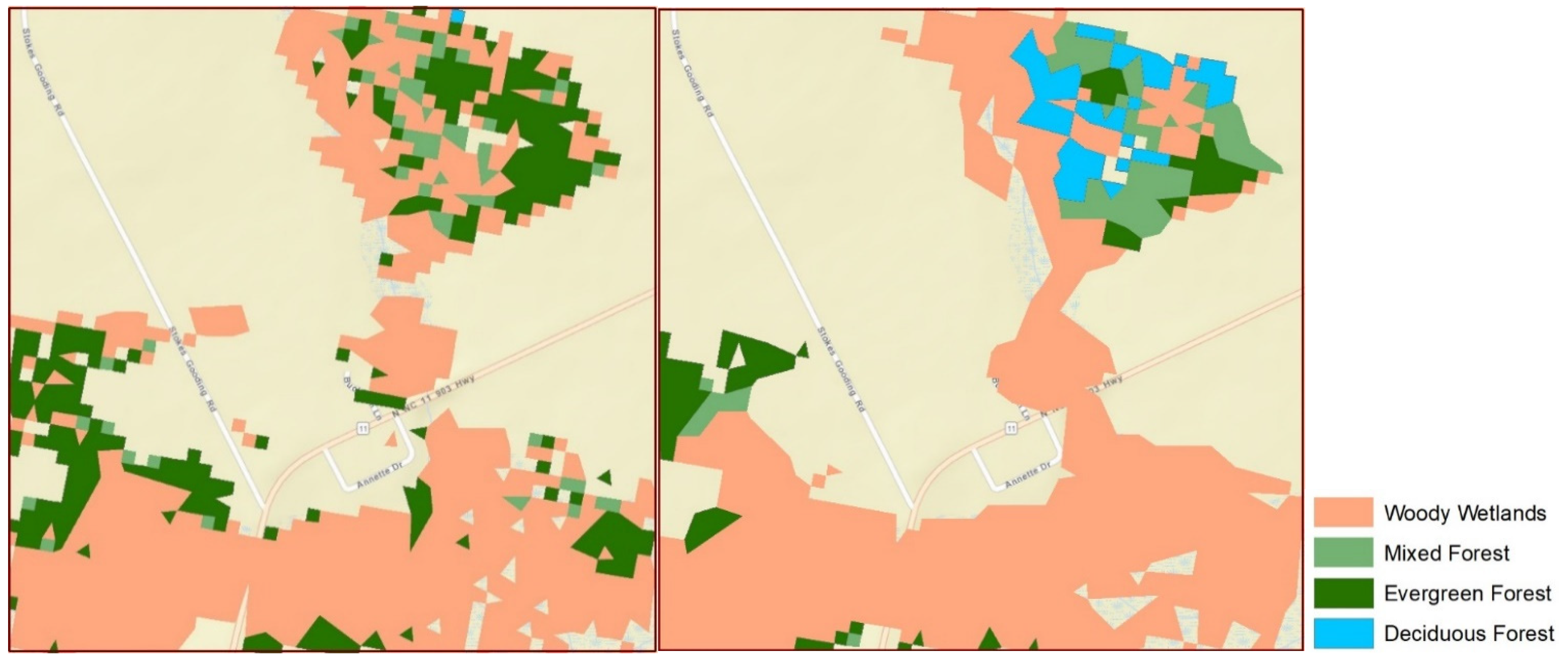
3.1. Land Cover Analysis

Both CDL and the NLCD provide raster-formatted land cover data. Each dataset is classified according to various land cover types, including barren land, water, forest land, and land used for agricultural purposes. Forestland is further broken down into four categories: deciduous forest, evergreen forest, mixed forest, and woody wetlands. The CDL and the NLCD define the four forest categories identically. Deciduous forest is defined as the areas dominated by trees generally greater than 5 m tall, greater than 20% of the total vegetation cover, and more than 75% of the tree species shedding foliage simultaneously in response to seasonal change. Evergreen forests are the areas dominated by trees greater than 5 m tall covering greater than 20% of the total vegetation cover with more than 75% of the tree species maintaining their leaves year-round. Mixed forests are areas with trees greater than 5 m tall and vegetation greater than 20%. Woody wetlands are areas where forest or shrubland vegetation accounts for greater than 20% of the vegetative cover and the soil or substrate is periodically saturated with or covered with water [27]. Because the definitions of the forest categories do not differ between the CDL and the NLCD, in this paper, we use the term CDL/NLCD forest types when referring to the deciduous forest, evergreen forest, mixed forest, and woody wetlands collectively.
In this study, CDL and the NLCD, are processed separately to provide two alternative spatial distributions of forest in the study area. While assessing the accuracy of either land cover map would be desirable, it would require the true land cover data, which we do not possess. Therefore, we only assess the degree to which the NLCD and CDL agree and disagree in identifying specific pixels as forests of alternative types.

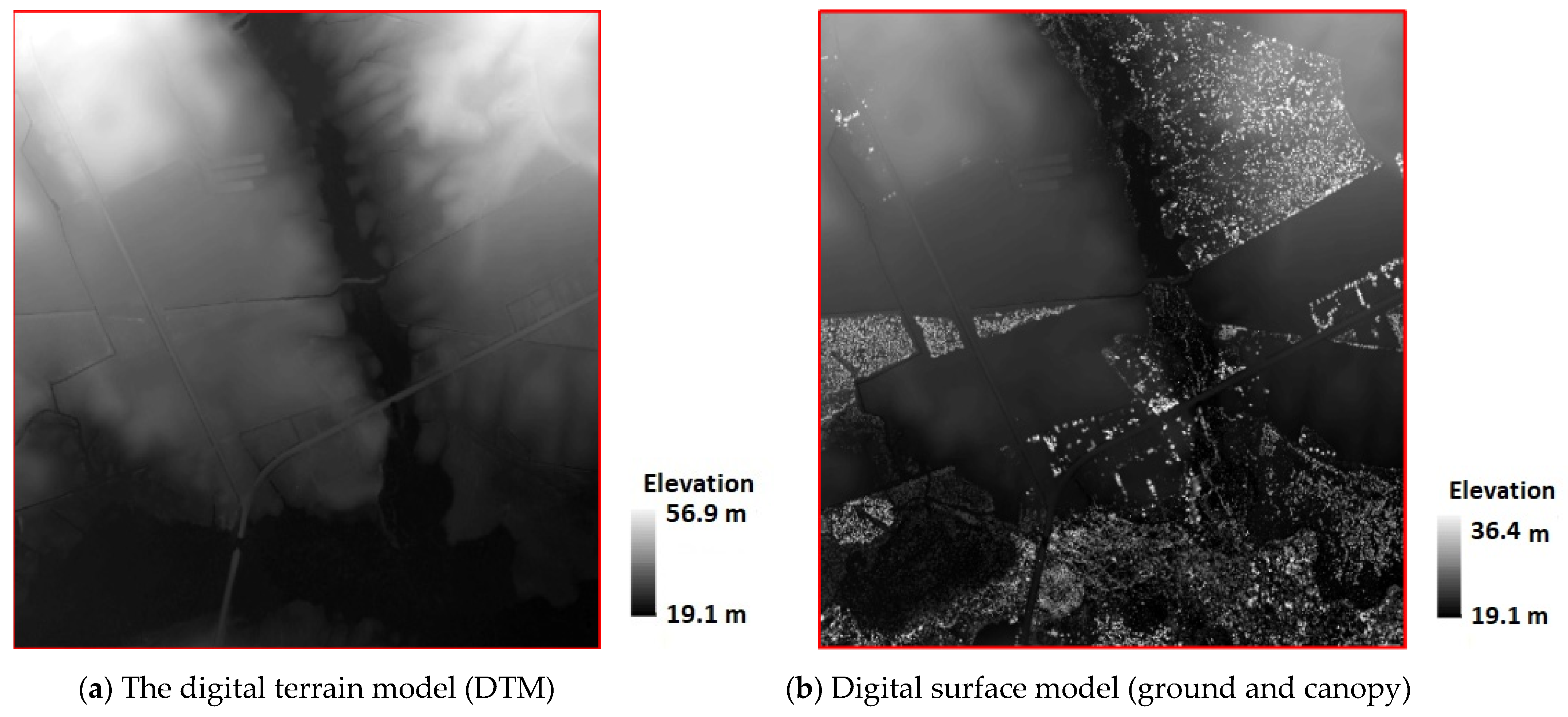
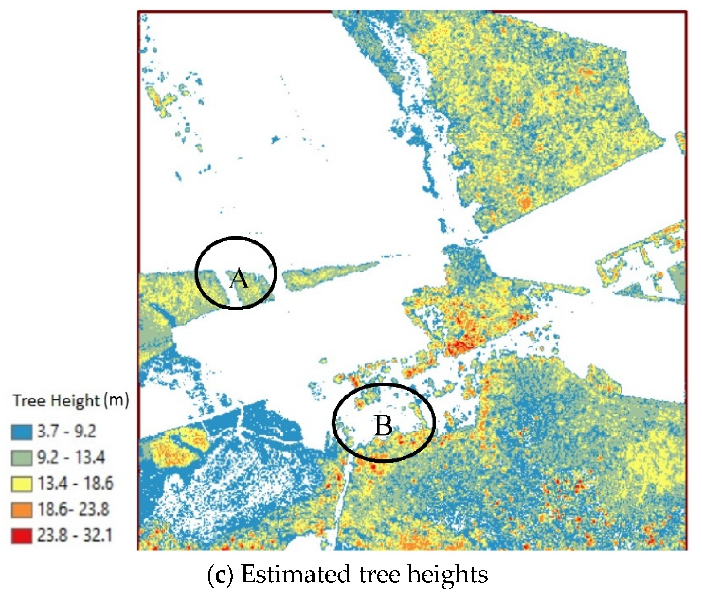
3.2. Tree Heights and LiDAR Analysis

Remote sensing has played an important role in biomass estimation and mapping across different spatial scales [29]. Numerous research studies have demonstrated the LiDAR’s ability to provide information that is useful for forest measurement, with the specific applications ranging from individual tree assessments to forest structure analysis and forest typing [30,31,32]. LiDAR data provides the direct measurement of three-dimensional structures and the underlying terrain and has been found useful for the detection of changes in forest areas due to both tree removal and growth. The canopy height information combined with stand density or canopy cover has been used for biomass estimation [33,34]. The challenges and performance of the methods to detect and delineate individual trees from LiDAR data are a subject of continuous research [35,36,37]. In this study, we apply a widely used method proposed by [38]. Under this approach, the LiDAR information is used to create the digital representations of two surfaces, ground and canopy, and the local high points in the canopy surface are regarded as representations of treetops. Tree heights are then estimated as the vertical difference between the canopy and the ground surfaces at the location of the treetops.
The ground surface or digital terrain model (DTM) is created from the LiDAR’s ground points, while vegetation and ground points are used for the canopy surface creation. For creating both surfaces a spline interpolation method is employed. The spline interpolation estimates the elevation of the surfaces at each point using a mathematical function (piecewise polynomial) that creates a smooth surface that passes exactly through the input points (LiDAR points) and minimizes the overall surface curvature. To obtain the treetop points, we employ the extended maxima transformation of the morphological image-analysis method that uses a local spatial search to identify the local high points in the canopy surface [38]. We apply different treetop identification thresholds recommended by this study, assess the results of each threshold visually at different scales (i.e., descriptive for the whole dataset and local comparisons for cell-by-cell), and select the ones that better match the LiDAR data and/or orthophoto available for the area. Then, a raster-based delineation model is applied to estimate the height of an individual tree as the difference between the Z coordinate of the treetop and the Z value of the DTM at the same X and Y position. Finally, each individual tree is assigned a forest type, i.e., deciduous, evergreen, mixed, or woody wetlands, by overlaying the CDL and the NLCD polygons on top of the canopy surface.

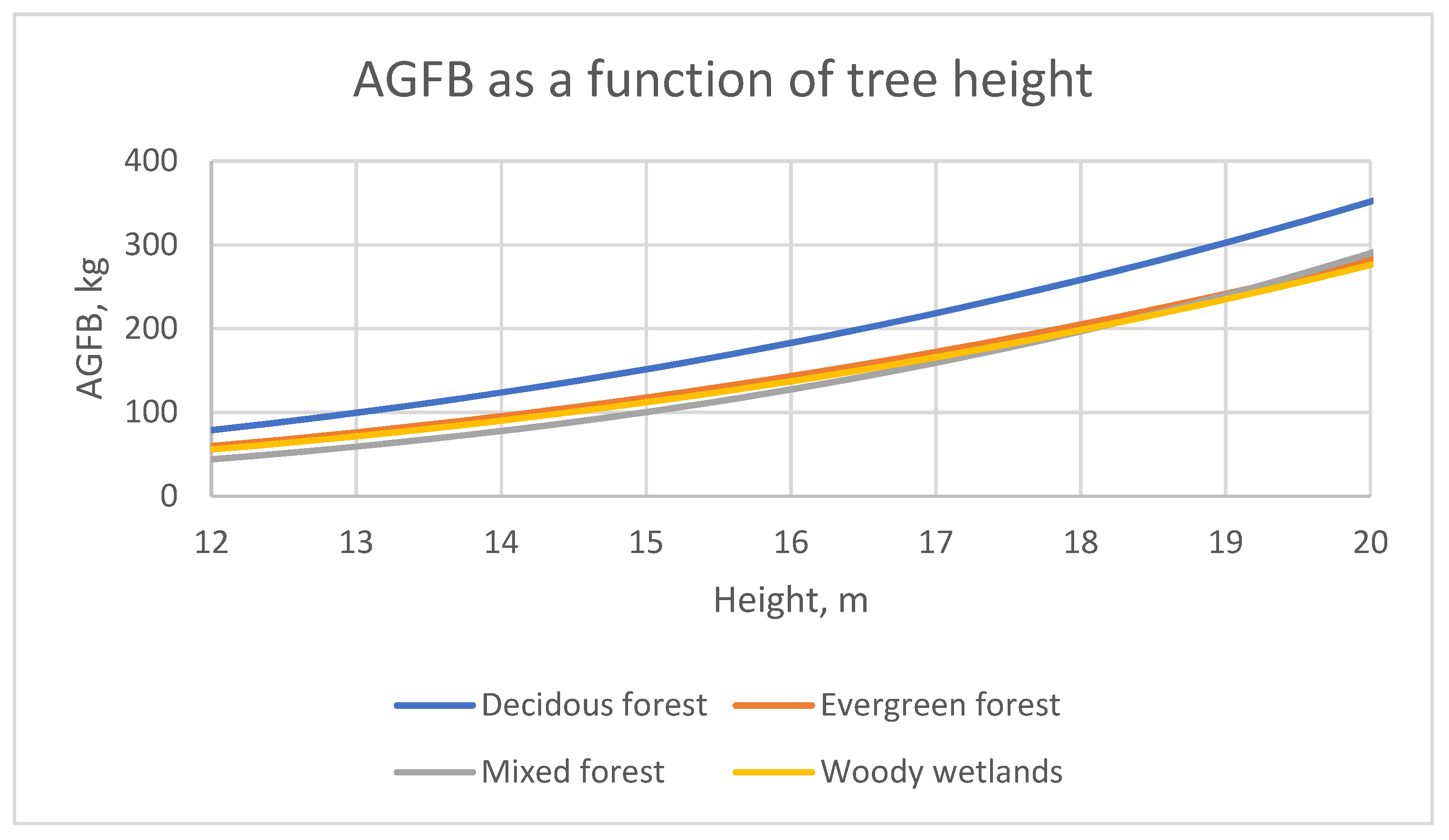
3.3. Tree Diameters and AGFB Estimation

We calculate the region-total AGFB as a sum of the AGFB of all of the individual trees in the region. Following the literature, we estimate the AGFB of individual trees as functions of their diameters [39]. Since LiDAR analysis provides the estimates of the heights of the trees, we begin with the estimation of the tree diameters as functions of their heights.
The standard measure of the diameter of a tree is the diameter at breast height (DBH), which is at 4.5 feet above the ground line [15]. The DBH–tree height (H) relationship varies with tree species, stand age, productivity, competition, and geography, and the functional form best describing this relationship is a subject of continuous research [40,41,42,43]. The topic of modeling DBH as a function of H has received renewed attention with the advancement of airborne laser scanning technologies that measure individual tree heights over large forest areas [44,45,46]. While no single DBH–H model is best for all applications, a log-linear functional form has been found to fit observational data and have desirable statistical properties [41,44,45,46]. Following this literature, we set:
ln(DBH) = α + β ln(H) + ε,
where DBH is in cm, H is in m, α and β are the parameters to be estimated, and ε is the standard linear regression error term. The scaling exponent β represents the ratio of the relative growth rate in DBH with respect to the relative growth rate in H [41]. We estimate four Equation (1), each corresponding to a specific CDL/NLCD forest type on a FIA sample matching the study area to the extent possible, as detailed below.
Because of the differences between the FIA and the CDL/NLCD data structures, two aspects of selecting the FIA sample data for estimating Equation (1) warrant a discussion: identification of the smallest FIA spatial unit containing the study area, and matching the four CDL/NLCD forest categories with FIA forest types. With respect to spatial units, the locations of the FIA plots on which individual trees have been measured are approximated. To preserve the privacy of landowners/managers, the actual FIA plot location could be different by up to 1.0 mile from the reported one. Additionally, up to 20% of the plot coordinates are swapped with another similar plot within the same county [15]. Thus, Duplin County is the smallest FIA spatial unit that entirely contains the study area. For that reason, in the estimation of Equation (1) we use only the tree measurements for the 2009–2013 FIA plots located in Duplin County.
With respect to forest categories, the FIA plots are assigned to specific forest types based on the tree species or species groups observed as dominating the location [15]. In contrast, the CDL and the NLCD group forests in more general categories, based on whether the trees in the location shed or do not shed leaves seasonally, and on whether the soils are or are not periodically saturated with water. To break the Duplin County FIA sample into the four sub-samples corresponding to the CLD/NLCD forest types we follow a two-step procedure. First, we use the species-defined FIA plot categorization to assign all of the trees on the plot to the deciduous, evergreen, or mixed forest based on whether the dominant species are deciduous, evergreen, or a combination of the two, respectively. For example, FIA plots of forest type 161 (loblolly pine) are dominated by evergreen species, loblolly pine, while FIA plots of forest type 708 (red maple/lowland) are dominated by deciduous species, red maple. Thus, for the estimation of Equation (1), we initially assign all the FIA trees from the plots of forest type 161 to the evergreen forest sub-sample, while the FIA trees from the plots of forest type 708 to the deciduous forest sub-sample.
In step two, we use the FIA plot information to determine whether to move some of the trees from their initial sub-samples to the woody wetlands sub-sample. Two cases are possible: the FIA forest type definition explicitly states that the forests in question typically occur on wet sites, or the definition allows for both wet and dry sites. In the first case, the corresponding tree observations are moved from the initially assigned sub-sample to the woody wetlands sub-sample. For example, the definition of FIA forest type 708 specifies, “Site—generally restricted to very moist to wet sites with poorly drained soils, and on swamp borders” [15]. Thus, for the estimation of Equation (1), we move all of the FIA trees from the plots of forest type 708 to the woody wetlands sub-sample. In the second case, we attribute the plot to woody wetlands if the plot site is reported as hydric (normally abundant or overabundant moisture all year), and leave the plot in the initial sub-sample if the plot site is not hydric, i.e., xeric (normally low or deficient in available moisture) or mesic (normally moderate but adequate available moisture) [15]. For example, the definition of the FIA forest type 161 allows for both hydric and non-hydric conditions: “Sites—upland soils with abundant moisture but good drainage, and on poorly drained depressions” [15]. Therefore, if the site of a FIA plot of this forest type is reported as hydric, we re-assign all of the FIA trees from this plot to the woody wetlands sub-sample. However, we keep the trees in the evergreen sample if the site of the plot is not hydric.
The AGFB of individual trees is estimated based on Jenkins biomass equations [15,38]. The equations are species-group-specific and are given by:
AGFB = exp (γ + δ ln(DBH)),
where the tree’s AGFB is in kg. Since, in our analysis, we do not observe individual tree species within the forest types, we chose the values of γ and δ corresponding to the tree species that define or dominate the specific CDL/NLCD forest type categories.
Once Equation (1) is substituted to Equation (2), we obtain the functional relationship between the tree height and the AGFB as:
AGFB = exp (γ + δα + δβ ln (H)).
Function (3) are used to calculate the AGFB of each tree measured by LiDAR analysis. The region-total AGFB is calculated as a sum of the estimated AGFB of all of the individual trees in the region.

4. Results

4.1. Comparison of CDL and NLCD

Table 1 summarizes the land cover data for Duplin County, as reported in the 2011 CDL and 2011 NLCD. We find a noticeable mismatch between the two datasets, suggesting some attributed inaccuracy in either or both datasets. Of particular interest for our application, we find that although the difference between the total forested land areas is 13%, the mismatch for the four specific forest categories is much higher. For example, when the entire Duplin County is considered, the evergreen forest area is estimated to be 35% higher, and the mixed forest area is estimated to be 83% lower according to the CDL when compared to the NLCD.
In the study area, the difference in the total forest area is relatively smaller than that in the county total, 102.7 ha in the CDL versus 101.0 ha in the NLCD, or 1.7%. The majority of the CDL forest land in the study area, 89%, is marked as forest land in the NLCD (Table 2). The same is true for the NLCD forestland: 91% of it is marked as forestland in the CDL (Table 2). The largest share of the mismatch is in shrubland, which is defined as areas dominated by young trees and shrubs that are less than 5 m tall [23].
For the 2.3 km2 study area, the mismatched forest land occurs mostly at the borders or edges of the forested land areas (Figure 3). While not the focus of this research, the study of edge or boundary effects in the field of GIS, especially at the intersection of raster data, remote sensing, and land cover analysis, is well-documented. Work by [30,47,48,49] has explored to what extent these boundary effects, essentially spatially-explicit problems, a result of arbitrary or discrete boundaries imposed on spatial data, have on the overall accuracy of land cover-based research.
Despite the total forest area estimates being close, there are notable differences between representations of the types of forest in the CDL and the NLCD in the study area (Figure 3).

4.2. Tree Heights and LiDAR Analysis

The results of LiDAR analysis are presented in Figure 4. As expected, the finer spatial resolution of the LiDAR data, approximately 0.3–0.5 m as opposed to the 30 m of the CDL and the NLCD, results in the LiDAR data identifying more areas with trees, when compared with either land cover maps. These differences are especially notable when tree cover is sparse, e.g., in the middle right-hand side of the maps.
For the purposes of the present analysis, the comparison of Figure 3 and Figure 4c reveals that differences in the CDL and the NLCD maps lead to some forested areas being included or not in the area-total AGFB estimates (e.g., area marked A in Figure 4c). Another result of the mismatch between the CDL and the NLCD maps is that there are forested areas that have different AGFB estimates because of the differences in the type of forest identified (e.g., area marked B in Figure 4c).
Tree heights (Figure 4c) are estimated as the vertical difference between the canopy surface (Figure 4b) and ground surface (Figure 4a) at the location of treetops. Area A contributes to the region-total AGFB estimate if CDL is used, but does not contribute if the NLCD is used. Area B’s contribution to the region-total AGFB differs between CDL, which identifies the forest as evergreen and woody wetlands, and the NLCD, which identifies the forest as woody wetlands only.

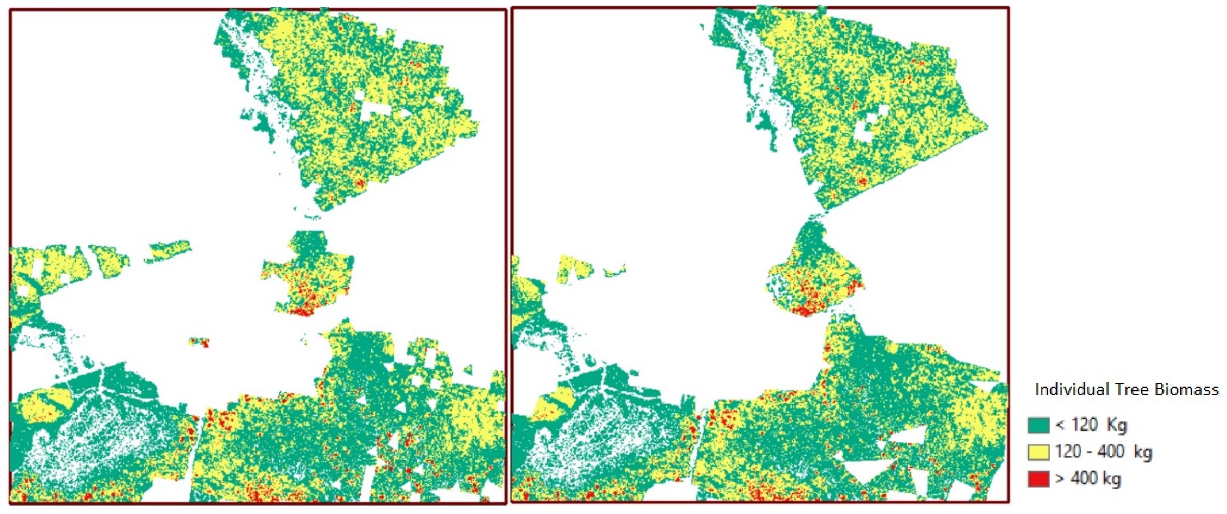
4.3. Tree Diameters and AGFB Estimation

Table 3 summarizes the breakdown of the 2009–2013 FIA sample for Duplin County, the data that we use for estimation of allometric Equation (1). While not exactly matching, the general breakdown of the Duplin County forests is compatible across the three datasets: CDL, NLCD, and FIA as all three datasets show that woody wetlands and evergreen forests dominate the area, followed by mixed and deciduous forests.
The summary of the diameter and height data used in the estimation of Equation (1) is provided in Table 4, and the results of the estimation are reported in Table 5.
All four models displayed a good statistical fit, as evidenced by the R2 ranging from 73% to 84% (Table 5), and all parameter estimates being statistically significant at conventional levels of significance.
Table 6 lists the parameter values used for Equation (2), by forest type, along with the original [39] species group names.
Figure 5 shows relationships (3) between the tree heights and the AGFB, which were developed by substituting Equation (1), which expresses tree diameter as a function of tree height, in Equation (2), which expresses the AGFB as a function of tree diameter. Even though Equation (2) does not differ between evergreen and mixed forests, Equation (1) does differ between these two forest types. In consequence, the AGFB function of tree height differs between evergreen and mixed forests.
The overall spatial distribution of the AGFB (Figure 6) closely follows the spatial distribution of tree heights (Figure 4), while also reflecting the differences in the location of forests as reported in the CDL and the NLCD (Figure 3).
We calculate the region-total AGFB as a sum of the AGFB of all of the individual trees in the region (Table 7). The main inputs of the biomass calculation, forest areas, and tree heights, are reported to facilitate the comparison and discussion of the results.

5. Discussion

Overall, we find that the two land cover maps agree in the qualitative description of the study region showing that woody wetlands and evergreen forests dominate the area, with mixed and deciduous forests occupying smaller portions. However, quantitatively, the CDL and the NLCD disagree on both the total forested area and on the forest composition. We find that the CDL-based forest area estimate is 13% higher than that based on the NLCD, but the area-total AGFB estimate derived with the NLCD is 22% higher than the CDL-based one. This difference points to the sensitivity of the area-total AGFB estimation to the breakdown of total forest land by type. One contributing factor for the higher NLCD-derived biomass estimate is that this land cover product identifies a larger portion of the area as deciduous forest. This, combined with the estimated tree height–AGFB relationship being higher for the deciduous forest when compared with the other three types considered (over a relevant range of tree heights) (Figure 5), results in higher NLCD-derived AGFB estimates for a relatively large, northeastern portion of the study area (Figure 3).
In addition to the potential errors in land cover classification, there are three other major sources of potential errors that can impact the AGFB estimates obtainable using our method: errors in the temporal mismatch of the three datasets used in the method (land use datasets, LiDAR, and data that goes in the estimation of DBH–height functions), errors in LiDAR estimates of tree heights, and errors in the DBH–height functions. For the proposed approach to work, LiDAR data would need to be collected at the same time as the land use maps. To minimize the impact of the temporal misalliance uncertainty, we match the years of the data to the extent that is possible, as detailed in Section 2. The specific method of estimation of tree heights from LiDAR data we use was chosen for its proven wide applicability and use. While other methods of tree height estimation might be better suited under specific situations [35,36,37], there is no indication that alternatively derived tree height estimates would have altered our main conclusion about the disagreement in the CDL and the NLCD impacting the area-total AGFB estimates.
We find that the fit of the models (1) quantifying the DBH–height relationship, as measured by R2, is on the lower side of the models presented in the literature. The reason for this tendency is that the majority of the models presented in the literature were estimated with a goal that was different from ours, namely, to show how the DBH–height relationship varies with tree species, stand age, productivity, competition, and/or differences in a geographic region [43,52,53,54,55]. In contrast with this literature, the purpose of the statistical estimation in our case is to only demonstrate that the DBH–height relationship could be reliably estimated from the publicly available FIA data. The data we use for the estimation of each of the four Equation (1) covers multiple species and/or narrowly defined forest types, as detailed in Table 3. This variety of species/forest types leads to greater variation in the tree DBH–height relationship within each of the four sub-samples when compared to the samples containing only a single tree species or a single narrowly defined forest type. Additionally, we model tree DBH as a function of a single independent variable; height. However, the relationship has also been modeled using plot or stand-level covariates to account for the influence of stand density or competition, and with accounting for the spatial correlation between observations [43,54]. Future research could extend our analysis in such a direction, contributing to the improved understanding of how the AGFB varies with tree height for different types of forests
Future applications of the biomass estimates obtained using our method could explore the economic potential and the environmental implications of harvesting the AGFB of specific forest types. We found that woody wetlands occupy a significant portion of Duplin County in general and the chosen study area in particular. The soil or substrate in such forests is periodically saturated with or covered with water. This provides an impetus to conduct additional analysis to evaluate what portion, if any, of the woody wetlands could be harvested in a cost-effective and environmentally sustainable manner.

6. Conclusions

This study introduced a new approach of combining the information available in land use maps and LiDAR data for the estimation of the AGFB and has highlighted the impact of the disagreement in widely available land use maps on AGFB estimates. We use the information from a FIA sample to develop study-region-specific allometric equations, but we are not aiming at improving FIA metrics. We view the proposed approach as a complementary way to obtain the AGFB estimates by combining the types of data (digital land use maps and LiDAR) that have not previously been used for such a purpose. The comparison of the accuracy of the traditional, FIA-based approach and our proposed approach on larger study areas is important but requires the concurrent LiDAR data that covers such larger areas that we do not have. Such a comparison constitutes an intriguing proposal for future research.
The approach we propose is a step towards supplementing sample-based regional AGFB estimates with the estimates based on the population representation of forests via remotely sensed land cover data. Continuing progress with the methodology design of the NLCD and CDL is contributing to the improved accuracy of the land cover data [55]. As the accuracy of the remotely sensed data improves with time, the contribution of the potential land cover data error to the AGFB estimation approach proposed is expected to decline.
With the advances in the new remote sensing technology and the availability of high spatial and temporal resolution of land use geospatial data, such combined use of multiple data sources opens up new possibilities for the proposed methodology. Both alternative land use map products and LiDAR datasets could be utilized in future applications. One of the promising map products comes from the Coastal Area Program (CAP), which develops land use maps at a 1 m resolution for the coastal U.S., and could be potentially expanded to the areas further inland. LiDAR data are presently being collected for the entire U.S. [56]. Complementing the traditional collection methods, the relatively new UAV technology could be used to obtain LiDAR data on-demand, thereby extending the possibilities for the applications of our approach.

Author Contributions

Conceptualization and methodology L.H.-B., L.A.K.; formal analysis L.H.-B., L.A.K.; investigation, L.A.K., L.H.-B., T.J.M., C.S.A.; data curation L.H.-B., L.A.K., C.S.A.; writing—original draft preparation L.A.K., L.H.-B., T.J.M. All authors have read and agreed to the published version of the manuscript.

Funding

Partial funding for the study has been provided by the Research Partnership Agreement 15-JV-11330143-010 between the USDA Forest Service and NCA&T, by NCDA&CS Bioenergy Research Initiative grant 19-026-4008; by Title III HBGI grant funded by the U.S. Department of Education; and by NSF grants 1800768 and 1824949. Any opinions, findings, and conclusions or recommendations expressed in this material are those of the author(s) and do not necessarily reflect the views of the U.S. Department of Agriculture, North Carolina Department of Agriculture and Consumer Services, U.S. Department of Education, and National Science Foundation.

Institutional Review Board Statement

Not applicable.

Informed Consent Statement

Not Applicable.

Conflicts of Interest

The authors declare no conflict of interest.

References

  1. Cartisano, R.; Mattioli, W.; Corona, P.; Mugnozza, G.; Sabatti, M.; Ferrari, B.; Cimini, D.; Giuliarelli, D. Assessing and mapping biomass potential productivity from poplar-dominated riparian forests: A case study. Biomass Bioenergy 2013, 54, 293–302. [Google Scholar] [CrossRef] [Green Version]
  2. Matasci, G.; Hermosilla, T.; Wulder, M.; White, J.; Coops, N.; Hobart, G.; Zald, H. Large-area mapping of Canadian boreal forest cover, height, biomass and other structural attributes using Landsat composites and lidar plots. Remote Sens. Environ. 2018, 209, 90–106. [Google Scholar] [CrossRef]
  3. U.S. Department of Energy (USDOE). 2016 Billion-Ton Report: Advancing Domestic Resources for a Thriving Bioeconomy, Volume 1: Economic Availability of Feedstocks; Langholtz, M.H., Stokes, N.J., Eaton, L.M., Eds.; ORNL/TM-2016/160; Oak Ridge National Laboratory: Oak Ridge, TN, USA, 2016; 448p. Available online: http://energy.gov/eere/bioenergy/2016-billion-ton-report (accessed on 7 July 2021). [CrossRef] [Green Version]
  4. Zhao, F.; Huang, C.; Goward, S.; Schleeweis, K.; Rishmawi, K.; Lindsey, M.; Denning, E. Development of Landsat-based annual US forest disturbance history maps (1986–2010) in support of the North American Carbon Program (NACP). Remote Sens. Environ. 2018, 209, 312–326. [Google Scholar] [CrossRef]
  5. Conrad, J.L., IV; Bolding, M.C.; Smith, R.L.; Aust, W.M. Wood-energy market impact on competition, procurement practices, and profitability of landowners and forest products industry in the U.S. south. Biomass Bioenergy 2011, 35, 280–287. [Google Scholar] [CrossRef]
  6. Abt, K.L.; Abt, R.C.; Galik, C.S.; Skog, K.E. Effect of Policies on Pellet Production and Forests in the U.S. South: A Technical Document Supporting the Forest Service Update of the 2010 RPA Assessment; General Technical Report SRS-202; U.S. Department of Agriculture, Southern Research Station: Ashville, NC, USA, 2014. [Google Scholar]
  7. Henderson, J.E.; Joshi, O.; Parajuli, R.; Hubbard, W. A regional assessment of wood resource sustainability and potential economic impact of the wood pellet market in the U.S. South. Biomass Bioenergy 2017, 105, 421–427. [Google Scholar] [CrossRef]
  8. Duden, A.S.; Verweij, P.A.; Junginger, H.M.; Abt, R.C.; Henderson, J.D.; Dale, V.H.; Kline, K.L.; Karssenberg, D.; Verstegen, J.A.; Faaij, A.P.C.; et al. Modeling the impacts of wood pellet demand on forest dynamics in southeastern United States: Modelling the impacts of wood pellet demand on forest dynamics in southeastern United States. Biofuels Bioprod. Biorefining 2017, 11, 1007–1029. [Google Scholar] [CrossRef] [Green Version]
  9. Abt, R.C.; Abt, K.L.; Cubbage, F.W.; Henderson, J.D. Effect of policy-based bioenergy demand on southern timber markets: A case study of North Carolina. Biomass Bioenergy 2010, 34, 1679–1686. [Google Scholar] [CrossRef]
  10. Prestemon, J.P.; Wear, D.N. Linking Harvest Choices to Timber Supply. Forest Sci. 2000, 46, 377–389. [Google Scholar]
  11. Caspersen, J.P.; Pacala, S.W.; Jenkins, J.C.; Hurtt, G.C.; Moorcroft, P.R.; Birdsey, R.A. Contributions of Land-Use History to Carbon Accumulation in U.S. Forests. Science 2000, 290, 1148–1151. [Google Scholar] [CrossRef]
  12. Galik, C.S.; Abt, B.; Wu, Y. Forest Biomass Supply in the Southeastern United States—Implications for Industrial Roundwood and Bioenergy Production. J. For. 2009, 107, 69–77. [Google Scholar]
  13. Polyakov, M.; Wear, D.N.; Huggett, R.N. Harvest Choice and Timber Supply Models for Forest Forecasting. Forest Sci. 2010, 56, 344–355. [Google Scholar]
  14. Brown, M.J.; Vogt, J.T. North Carolina’s Forests, 2013; Resource Bulletin SRS-2015; U.S. Department of Agriculture, Southern Research Station: Ashville, NC, USA, 2015. [Google Scholar]
  15. Burrill, E.A.; Wilson, A.M.; Turner, J.A.; Pugh, S.A.; Menlove, J.; Christiansen, G.; Conkling, B.L.; David, W. The Forest Inventory and Analysis Database: Database Description and User Guide Version 7.2 for Phase 2; U.S. Department of Agriculture, Forest Service: Washington, DC, USA, 2017; p. 946. Available online: http://www.fia.fs.fed.us/library/database-documentation/ (accessed on 7 July 2021).
  16. Lister, A.J.; Andersen, H.; Frescino, T.; Gatziolis, D.; Healey, S.; Heath, L.S.; Liknes, G.C.; McRoberts, R.; Moisen, G.G.; Nelson, M.; et al. Use of Remote Sensing Data to Improve the Efficiency of National Forest Inventories: A Case Study from the United States National Forest Inventory. Forests 2020, 11, 1364. [Google Scholar] [CrossRef]
  17. Liknes, G.C.; Nelson, M.D.; Gormanson, D.D.; Hansen, M. The Utility of the Cropland Data Layer for Forest Inventory and Analysis, Proceedings of the Eighth Annual Forest Inventory and Analysis Symposium, Monterey, CA, USA, 16–19 October 2006; McRoberts Ronald, E., Reams Gregory, A., Van Deusen Paul, C., McWilliams William, H., Eds.; Gen. Tech. Report WO-79; US Department of Agriculture, Forest Service: Washington, DC, USA, 2006; Volume 79, pp. 259–264. [Google Scholar]
  18. Chen, X.; Liu, S.; Zhu, Z.; Vogelmann, J.; Li, Z.; Ohlen, D. Estimating aboveground forest biomass carbon and fire consumption in the U.S. Utah High Plateaus using data from the Forest Inventory and Analysis Program, Landsat, and LANDFIRE. Ecol. Indic. 2011, 11, 140–148. [Google Scholar] [CrossRef]
  19. Ahamed, T.; Tian, L.; Zhang, Y.; Ting, K.C. A review of remote sensing methods for biomass feedstock production. Biomass Bioenergy 2011, 35, 2455–2469. [Google Scholar] [CrossRef]
  20. Rosette, J.; Suarez, J.; Nelson, R.; Los, S.; Cook, B.; North, P. LiDAR Remote Sensing for Biomass Assessment. Remote Sens. Biomass 2012, 3–21. [Google Scholar] [CrossRef] [Green Version]
  21. Zhen, Z.; Quackenbush, L.J.; Zhang, L. Trends in automatic individual tree crown detection and delineation—Evolution of LiDAR data. Remote Sens. 2016, 8, 333. [Google Scholar] [CrossRef] [Green Version]
  22. Lu, D.; Chen, Q.; Wang, G.; Liu, L.; Li, G.; Moran, E. A survey of remote sensing-based aboveground biomass estimation methods in forest ecosystems. Int. J. Digit. Earth 2016, 9, 63–105. [Google Scholar] [CrossRef]
  23. McRoberts, R.E.; Næsset, E.; Gobakken, T. Inference for LiDAR-assisted estimation of forest growing stock volume. Remote Sens. Environ. 2013, 128, 268–275. [Google Scholar] [CrossRef]
  24. Nelson, R.; Margolis, H.; Montesano, P.; Sun, G.; Cook, B.; Corp, L.; Andersen, H.-E.; DeJong, B.; Pellat, F.P.; Fickel, T.; et al. LiDAR-based estimates of aboveground biomass in the continental US and Mexico using ground, airborne, and satellite observations. Remote Sens. Environ. 2017, 188, 127–140. [Google Scholar] [CrossRef] [Green Version]
  25. McRoberts, R.E.; Liknes, G.C.; Domke, G.M. Using a remote sensing-based, percent tree cover map to enhance forest inventory estimation. Forest Ecol. Manag. 2014, 331, 12–18. [Google Scholar] [CrossRef]
  26. U.S. Department of Agriculture, National Agricultural Statistics Service (USDA/NASS). Cropland Data Layer; Published Crop-specific Data Layer; USDA-NASS: Washington, DC, USA, 2020. Available online: https://nassgeodata.gmu.edu/CropScape/ (accessed on 5 May 2018).
  27. Multi-Resolution Land Characteristics Consortium (MRLC). National Land Cover Database. 2020. Available online: https://www.mrlc.gov/data-services-page (accessed on 5 May 2018).
  28. Thomas, V.A.; Wynne, R.H.; Kauffman, J.; McCurdy, W.; Brooks, E.B.; Thomas, R.Q.; Rakestraw, J. Mapping thins to identify active forest management in southern pine plantations using Landsat time series stacks. Remote Sens. Environ. 2021, 252, 112127. [Google Scholar] [CrossRef]
  29. Kumar, L.; Mutanga, O. Remote sensing of above-ground biomass. Remote Sens. 2017, 9, 935. [Google Scholar] [CrossRef] [Green Version]
  30. Kumari, R.; Smith, A. Remote Sensing Based Forest Fragmentation Analysis Using GIS along Fringe Forests of Kollam District, Kerala. Int. J. Res. Appl. Sci. Eng. Technol. 2017, 728–739. [Google Scholar] [CrossRef]
  31. Zhang, C.; Zhou, Y.; Qiu, F. Individual tree segmentation from LiDAR point clouds for urban forest inventory. Remote Sens. 2015, 7, 7892–7913. [Google Scholar] [CrossRef] [Green Version]
  32. Wiggins, H.L.; Nelson, C.R.; Larson, A.J.; Safford, H.D. Using LiDAR to develop high-resolution reference models of forest structure and spatial pattern. Forest Ecol. Manag. 2019, 434, 318–330. [Google Scholar] [CrossRef]
  33. Liu, J.; Shen, J.; Zhao, R.; Xu, S. Extraction of individual tree crowns from airborne LiDAR data in human settlements. Math. Comput. Model. 2013, 58, 524–535. [Google Scholar] [CrossRef]
  34. García, M.; Riaño, D.; Chuvieco, E.; Danson, F.M. Estimating biomass carbon stocks for a Mediterranean forest in central Spain using LiDAR height and intensity data. Remote Sens. Environ. 2010, 114, 816–830. [Google Scholar] [CrossRef]
  35. Chen, W.; Xiang, H.; Moriya, K. Individual tree position extraction and structural parameter retrieval based on airborne LiDAR data: Performance evaluation and comparison of four algorithms. Remote Sens. 2020, 12, 571. [Google Scholar] [CrossRef] [Green Version]
  36. Yun, T.; Jiang, K.; Li, G.; Eichhorn, M.P.; Fan, J.; Liu, F.; Cao, L. Individual tree crown segmentation from airborne LiDAR data using a novel Gaussian filter and energy function minimization-based approach. Remote Sens. Environ. 2021, 256, 112307. [Google Scholar] [CrossRef]
  37. Chen, X.; Jiang, K.; Zhu, Y.; Wang, X.; Yun, T. Individual tree crown segmentation directly from UAV-borne LiDAR data using the PointNet of deep learning. Forests 2021, 12, 131. [Google Scholar] [CrossRef]
  38. Kwak, D.A.; Lee, W.K.; Lee, J.H.; Biging, G.S.; Gong, P. Detection of individual trees and estimation of tree height using LiDAR data. J. Forest Res. 2007, 12, 425–434. [Google Scholar] [CrossRef]
  39. Jimenez-Berni, J.A.; Deery, D.M.; Rozas-Larraondo, P.; Condon, A.T.G.; Rebetzke, G.J.; James, R.A.; Sirault, X.R. High throughput determination of plant height, ground cover, and above-ground biomass in wheat with LiDAR. Front. Plant Sci. 2019, 9, 237. [Google Scholar] [CrossRef] [Green Version]
  40. Yuancai, L. Remarks on Height-Diameter Modeling; US Department of Agriculture, Forest Service, Southern Research Station: Asheville, NC, USA, 2001. [Google Scholar]
  41. Niklas, K.J. Plant allometry: Is there a grand unifying theory? Biol. Rev. 2004, 79, 871–889. [Google Scholar] [CrossRef] [PubMed]
  42. Lhotka, J.M. Height-diameter relationships in Sweetgum (Liquidambar styraciflua)-dominated stands. South. J. Appl. For. 2012, 36, 98–106. [Google Scholar] [CrossRef]
  43. Saud, P.; Lynch, T.B.; KC, A.; Guldin, J.M. Using quadratic mean diameter and relative spacing index to enhance height–diameter and crown ratio models fitted to longitudinal data. Forestry 2016, 89, 215–229. [Google Scholar] [CrossRef] [Green Version]
  44. Bi, H.; Fox, J.C.; Li, Y.; Lei, Y.; Pang, Y. Evaluation of nonlinear equations for predicting diameter from tree height. Can. J. Forest Res. 2012, 42, 789–806. [Google Scholar] [CrossRef]
  45. Cao, Q.V.; Dean, T.J. Predicting diameter at breast height from total height and crown length. In Proceedings of the 15th Biennial Southern Silvicultural Research Conference; Guldin, J.M., Ed.; e-Gen. Tech. Rep. SRS-GTR-175; US Department of Agriculture, Forest Service, Southern Research Station: Asheville, NC, USA, 2013; Volume 175, pp. 201–205. [Google Scholar]
  46. Pascual, A. Using tree detection based on airborne laser scanning to improve forest inventory considering edge effects and the co-registration factor. Remote Sens. 2019, 11, 2675. [Google Scholar] [CrossRef] [Green Version]
  47. Holdt, B.; Civco, D.L.; Hurd, J. Forest fragmentation due to land parcelization and subdivision: A remote sensing and GIS analysis. In Proceedings of the 2004 ASPRS Annual Convention, Denver, CO, USA, 23–28 May 2004. [Google Scholar]
  48. Broadbent, E. Forest fragmentation and edge effects from deforestation and selective logging in the Brazilian Amazon. Biol. Conserv. 2008, 140, 142–155. [Google Scholar] [CrossRef]
  49. Ting, Z.; Shaolin, P. Spatial scale types and measurement of edge effects in ecology. Acta Ecol. Sin. 2008, 28, 3322–3333. [Google Scholar] [CrossRef]
  50. Holmes, J.S. Common Forest Trees of North Carolina (Revised), 12th ed.; North Carolina Department of Agriculture and Consumer Services, North Carolina Forest Service: Raleigh, NC, USA, 2012. [Google Scholar]
  51. Jenkins, J.C.; Chojnacky, D.C.; Heath, L.S.; Birdsey, R.A. National scale biomass estimators for United States tree species. Forest Sci. 2003, 49, 12–35. [Google Scholar]
  52. Henry, H.A.L.; Aarssen, L.W. The interpretation of stem diameter–height allometry in trees: Biomechanical constraints, neighbour effects, or biased regressions? Ecol. Lett. 1999, 2, 89–97. [Google Scholar] [CrossRef]
  53. Gonzalez-Benecke, C.A.; Gezan, S.A.; Martin, T.A.; Cropper, W.P., Jr.; Samuelson, L.J.; Leduc, D.J. Individual tree diameter, height, and volume functions for longleaf pine. Forest Sci. 2014, 60, 43–56. [Google Scholar] [CrossRef] [Green Version]
  54. Meng, Q.; Cieszewski, C.J.; Strub, M.R.; Borders, B.E. Spatial regression modeling of tree height–diameter relationships. Can. J. For. Res. 2009, 39, 2283–2293. [Google Scholar] [CrossRef]
  55. Jin, S.; Homer, C.; Yang, L.; Danielson, P.; Dewitz, J.; Li, C.; Zhu, Z.; Xian, G.; Howard, D. Overall methodology design for the United States national land cover database 2016 products. Remote Sens. 2019, 11, 2971. [Google Scholar] [CrossRef] [Green Version]
  56. What Is Lidar Data and Where Can I Download It? Available online: https://www.usgs.gov/faqs/what-lidar-data-and-where-can-i-download-it?qt-news_science_products=0#qt-news_science_products (accessed on 8 July 2021).
Figure 1. Location of the study area in North Carolina, Duplin County.
Remotesensing 13 02731 g001
Figure 2. Schematics of the analysis. Symbols: ovals—start/end; parallelogram—input or output; rectangle—process.
Remotesensing 13 02731 g002
Figure 3. Study area: Location of different types of forest as reported in CDL (left panel) and NLCD (right panel).
Remotesensing 13 02731 g003
Figure 4. Study area: (a) ground surface or DTM, (b) digital surface model, (c) tree heights. A and B are the examples of the areas within the study region for which the contribution to the region-total AGFB differs depending on whether CDL- or NLCD-based maps are used.
Remotesensing 13 02731 g004aRemotesensing 13 02731 g004b
Figure 5. Duplin County: Relationship between tree height and AGFB, by forest type.
Remotesensing 13 02731 g005
Figure 6. Study area: Spatial distribution of AGFB based on CDL (left panel) and NLCD (right panel).
Remotesensing 13 02731 g006
Table 1. Duplin County land cover: CDL and NLCD comparison.
Land CoverCDLNLCDArea Difference between CDL and NLCD, % 3
Code(s) 1HectaresCode(s) 2Hectares
Water92, 111765 11766 0%
Developed land121, 122, 123, 1248894 21, 22, 23, 249472−6%
Barren land13160 31702 −169%
Shrubland15228,567 5227,274 5%
Grassland, hay and pasture37, 17618,602 71, 818875 71%
Cultivated cropsMultiple 456,517 8275,728 −29%
Herbacious wetlands195703 953890 −139%
Total for land cover other than forest 114,108 126,707−10%
Deciduous Forest141179 41329 −59%
Evergreen Forest14245,838 4232,182 35%
Mixed Forest1432933 437061 −83%
Woody Wetlands19048,583 9046,157 5%
Total for forested land 97,533 85,729 13%
In Table 1 Codes, 1,2 for CDL and NLCD are adopted from USDA/NASS (2021) and MRLC (2021). For each category with the CDL area, aCDL, and NLCD area, aNLCD, the area difference, 3 is calculated (aCDL − aNLCD) × 2/(aCDL + aNLCD) × 100%. The area total of 26 categories was also calculated for “Multiple” 4 code.
Table 2. Study area: NLCD and CDL comparison; pixel count in alternative land cover.
CDLTotal
Deciduous ForestEvergreen ForestMixed ForestWoody WetlandsShrublandHerbaceous WetlandsCultivated CropsOther
NLCDDeciduous Forest0151539300072
Evergreen Forest073313501095
Mixed Forest0391331701192
Woody Wetlands01192762973933863
Shrubland11213458088122
Herbaceous Wetlands01311812035079
Cultivated Crops0421058082067961
Other0102877127124294
Total127662802223169952032578
The dark green cells correspond to the forest areas that are identified of the same forest type in both CDL and NLCD. These areas contribute the same amount to the region-total AGFB estimate irrespective of the land cover map used. The light green cells correspond to the areas that are identified as forests in both CDL and NLCD, but of different types. These areas contribute to the region-total AGFB estimate, but the contributions differ between the land cover maps because of the difference in forest type. The yellow cells correspond to the areas that are identified as forest in one and only one of the two datasets. These areas contribute or not to the region-total AGFB estimate depending on which of the cover maps is used. The cells without shading correspond to the areas that are identified as non-forest in both datasets. The non-forest categories are listed in italics. These areas do not contribute to the region-total AGFB estimate irrespective of the land cover map used.
Table 3. FIA vs. CDL/NLCD forest types: Duplin County, individual tree data from the 2009–2013 FIA.
FIA Forest TypeCDL/NLCD Forest Type AssignedTree Count **
Code and Name *Description of Typical Sites *Hydric Site? ** Yes or No
161—Loblolly pineSites—upland soils with abundant moisture but good drainage, and on poorly drained depressions.NoEvergreen848
YesWoody wetlands15
166—Pond pineSites—rare, but found in southern New Jersey, Delaware, and Maryland in low, poorly drained acres, swamps, and marshes.YesWoody wetlands89
406—Loblolly pine/hardwoodSites—usually moist to very moist though not wet all year, but also on drier sites.NoMixed161
508—Sweetgum/yellow-poplarSites—generally occupies moist, lower slopes.NoWoody wetlands41
YesWoody wetlands29
519—Red maple/oakSites—uplands.NoDeciduous77
608—Sweetbay/swamp tupelo/red mapleSites—very moist but seldom wet all year shallow ponds, muck swamps, along smaller creeks in Coastal Plain.NoWoody wetlands254
YesWoody wetlands94
708—Red maple/lowlandSite—generally restricted to very moist to wet sites with poorly drained soils, and on swamp borders.NoWoody wetlands23
Total observations1631
Notes: * Source of information: FIA database manual [15]. For the descriptions and visual references on the tree species, sites, and forest types see [14,50], and www.ncwetlands.org, accessed on 1 June 2021, ** Source of information: FIA data.
Table 4. FIA 2009–2013 Duplin County sample: Summary statistics.
Variable, Units of MeasurementStatisticNLCD/CDL Forest Type, Number of Observations
Deciduous Forest,
77 obs.
Evergreen Forest,
848 obs.
Mixed Forest,
161 obs.
Woody Wetlands,
545 obs.
DBH, cmMean16.316.915.118.3
Median15.716.514.016.0
Minimum2.82.52.52.5
Maximum62.547.855.172.1
Standard deviation9.08.111.812.3
H, mMean12.812.511.914.1
Median14.312.811.013.4
Minimum4.03.43.42.1
Maximum21.625.935.137.5
Standard deviation4.34.96.26.5
Table 5. Estimated tree diameters (DBH)–tree height (H) functions (1).
VariableNLCD/CDL Forest Type, Number of Observations
Deciduous Forest,
77 obs.
Evergreen Forest,
848 obs.
Mixed Forest,
161 obs.
Woody Wetlands,
545 obs.
Constant, α−0.421
(0.176)
−0.380
(0.065)
−1.168
(0.126)
−0.522
(0.073)
Height, β1.238
(0.070)
1.248
(0.026)
1.515
(0.052)
1.263
(0.028)
R20.810.730.840.78
Note: Standard errors in parentheses. The estimate of α for deciduous forest is statistically significant at a 5% level of significance, and all other parameter estimates are statistically different from zero at a 1% level of significance.
Table 6. Parameters of AGFB (B)—tree diameters (DBH) functions (2).
Forest TypeγδBurrill et al. (2017) Species [15]Jenkins (2003) Species Group [51]
Deciduous−1.91232.3651Red oak, mapleSoft maple/birch
Evergreen−2.53562.4349Loblolly pine, pond pinePine
Mixed−2.53562.4349Loblolly pinePine
Woody wetlands−2.482.4835Sweetbay, swamp tupeloMixed hardwood
Table 7. Study-region total AGFB estimates.
Forest TypeCDLNLCD
Total Area (ha)Avg. Tree Height (m)Total B (kg)Total Area (ha)Avg. Tree Height (m)Total B (kg)
Decidious0.115.2415,8806.516.63,977,151
Evergreen24.816.6810,882,7038.516.533,192,142
Mixed5.614.131,083,4628.315.212,238,870
Woody Wetland72.216.9131,776,53077.718.3245,428,628
Total102.7 101 54,836,791
Publisher’s Note: MDPI stays neutral with regard to jurisdictional claims in published maps and institutional affiliations.

