Abstract
Satellite images are always partitioned into regular patches with smaller sizes and then individually fed into deep neural networks (DNNs) for semantic segmentation. The underlying assumption is that these images are independent of one another in terms of geographic spatial information. However, it is well known that many land-cover or land-use categories share common regional characteristics within a certain spatial scale. For example, the style of buildings may change from one city or country to another. In this paper, we explore some deep learning approaches integrated with geospatial hash codes to improve the semantic segmentation results of satellite images. Specifically, the geographic coordinates of satellite images are encoded into a string of binary codes using the geohash method. Then, the binary codes of the geographic coordinates are fed into the deep neural network using three different methods in order to enhance the semantic segmentation ability of the deep neural network for satellite images. Experiments on three datasets demonstrate the effectiveness of embedding geographic coordinates into the neural networks. Our method yields a significant improvement over previous methods that do not use geospatial information.
1. Introduction
Waldo Tobler’s first law of geography [1] says, “everything is related to everything else, but near things are more related than distant things.” Satellite images are snapshots of the Earth’s surface. Therefore, semantic labels of these images are also in agreement with Waldo Tobler’s first law of geography. This means that near satellite images share some common latent patterns and distant satellite images are quite different from one another. For instance, as shown in Figure 1a,b, buildings from different cities are diverse in terms of color, size, morphological structure and density. It can be seen from Figure 2a that each city in this figure has its own regularity. However, this kind of geospatial distribution is difficult to describe and quantify using features from an image patch with a rather small size. Thus, in previous studies, parts of these patterns have been expressed as region-specific configurations or models [2,3,4,5]. Instead of manually building region-specific configurations, we resort to powerful DNNs to automatically learn the regional similarity and diversity of large-scale data from geographic coordinates. Geographic coordinates are one of the most notable characteristics of satellite images, which have been omitted in previous studies. To the best of our knowledge, this is the first attempt to map high-resolution satellite images on a large scale by modeling their geographic coordinates.
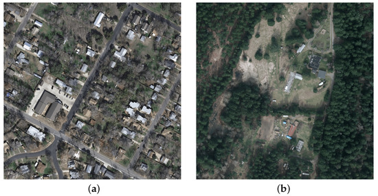
Figure 1.
Images from the Inria Aerial Image dataset [6]; (a,b) are sample images from the city of Austin and Kitsap County in the U.S.
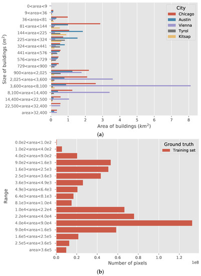
Figure 2.
Building areas of five cities from the Inria building dataset: (a) plots the building size with respect to each city. The units of the building size in this figure are m2 and km2. The distributions of the building size are quite diverse in these cities. It should be noted that the intervals of building size are not divided evenly; (b) plots the building size of the entire dataset using the number of pixels as the unit. The values are calculated based on the ground truth of the dataset. Most of the buildings are smaller than 250,000 pixels (). Therefore, the image tiles are divided into patches with a size of when training.
Geospatial information is often involved in the global mapping process of widely distributed satellite images. At global-scale mapping, the heterogeneity of the data makes it unfeasible to describe them using a uniform model. A common idea for handling this problem is to partition the entire world into several regions. Based on local similarities, an index-based method [2] selects a region-specific threshold for each region. Similarly, classifier-based methods train a classifier for each area with region-specific parameters [3,4]. For the interactive method [5], knowledge-based verification is attached to different areas after classification. Global low-resolution reference data can also be used as an indicator to overcome the heterogeneity in datasets [7]. Weighting samples by frequency has been adopted to mitigate the class imbalance among different cities [8]. All of these methods can enable the model to appropriately capture the regional pattern of the data, which is accomplished by using region-specific configurations based on experts’ experiences.
In this paper, rather than directly dividing the dataset into multiple groups, we aim to learn the regional characteristics using DNNs. This is accomplished by feeding DNNs with binary codes converted from the geographic coordinates of the images. The essential conversion builds on the idea of the geohash method [9], which was invented for retrieving and locating image tiles [7,10,11,12,13]. It should be noted that the geohash code is just a type of geographical coordinate. Readers should not confuse this term with the hash code used in cryptography. In cryptography, a hash function must satisfy the following requirements: uniformity property, uniqueness property, second pre-image resistance and collision resistance. The method called “geohash codes” in this paper does not satisfy these requirements, thus the “geohash codes” used in geography are quite different from hash codes used in cryptography. The closer two positions are, the more bits of geocodes they share. There are a few existing studies on using geospatial coordinates to improve the model performance of different applications [14,15,16]. The GPS encoding feature [14] converts geospatial coordinates into the code of grid cells, which is a special type of one-hot encoding in essence. It incorporates location features by adding a concatenate layer to boost the accuracy of image classification. Geolocation can also be a benefit for predicting dialect words via mixture density networks [15]. The input features of the mixture density network are purely latitude and longitude coordinates without any other features, and the model output dialect words with given geospatial coordinates. Disaster assessment is another practical application scenario [16]. It employs the pre-trained DNNs for the feature extraction of flooding images. Then these image features, along with the latitude and longitude coordinates, are used for training other machine learning models, such as random forest, logistic regression, multilayer perceptron and support vector machine. In this paper, the geocodes, generated by the geohash method, embed the spatial information into models to assist in the semantic segmentation. Essentially, the geohash method is a special type of binary space partitioning. It converts the decimal coordinates of longitude and latitude into binary numbers. Both decimal and binary numbers can represent an accurate position, but the binary geocode is more convenient for controlling the code length. With extra geospatial information, the geohash codes increase the distinguishability of the model. Regulating the length of the binary code can force certain areas to share the same geocode. Thus, adjusting the code length can keep the model from suffering from a risk of overfitting.
To validate the effectiveness of our proposed method, we apply it to the task of semantic segmentation using DNNs. Semantic segmentation with DNNs has produced remarkable results in recent years. Different from the conventional methods for image segmentation [17,18,19,20,21,22], DNNs can learn rich semantic features in an end-to-end manner, which requires large-scale data. However, the demand for large-scale data is not involved in conventional segmentation methods, but this also limits their generalization performance. Most of the conventional segmentation methods utilize low-level features to extract objects of images, while deep learning approaches build hierarchical semantic features with numerous layers. The use of a fully convolutional network (FCN) [23] is the first work that trains convolutional neural networks (CNNs) for semantic segmentation in an end-to-end way. The input image of an FCN can be an arbitrary size, combining the feature maps at different resolutions via skip connections. A deconvolutional network [24] is proposed to recover the original size of the input images. U-Net [25] is an extension of the FCN, the upsampling parts of which are composed of deconvolutional layers. Dilated convolution [26,27] expands the receptive field of the convolutional layers and retains the high resolution of the feature maps. Atrous Spatial Pyramid Pooling (ASPP) [28] captures multi-scale context information with various dilation rates. The Pyramid Scene Parsing Network (PSPNet) [29] pools at various scales to better extract the global context information. These approaches have significantly improved the prediction results of semantic segmentation. There are plenty of previous works that focus on the semantic segmentation of high-resolution satellite images using DNNs, such as [30,31,32,33]. The datasets employed in these works virtually cover one or two cities [30,31]. When facing the challenge of covering more cities [32,33], the performance of the deep neural network fluctuates in different regions.
In most cases, the automatic extraction of a representation requires large-scale and widely distributed datasets. The prevalence of DNNs has resulted in the emergence of large-scale remote sensing datasets, such as AID [34], NWPU-RESISC45 [35], the ISPRS 2D Semantic Labeling Benchmark [36] and DOTA [37]. The sizes of these datasets are much larger than before, and their samples have been widely selected from around the world. Unfortunately, the rich information of the geospatial location is eliminated when building these datasets. Without attaching geographic coordinates, they are only treated as ordinary photos. As we focus on the semantic segmentation of high-resolution satellite images, the Inria Aerial Image dataset [6] and the Gaofen Image Dataset (GID) [38] are the only publicly available high-resolution datasets that retain the geographic coordinates for each image tile. These two datasets provide us with an opportunity to explore the influence of embedding geospatial information into DNNs. Additionally, we have built a worldwide dataset, called the Building dataset for Disaster Reduction and Emergence Management (DREAM-B), to further validate the proposed method. Figure 3 shows the spatial distributions of the three datasets.

Figure 3.
Distributions of the datasets: (a) distribution of the image tiles in the GID dataset [38] around China. Each point in this figure is one image tile. It contains 150 tiles in total. The training and test data are similarly distributed; (b) spatial distribution of the Inria building dataset [6]. Different from the GID dataset, each point in this figure is one city with 36 image tiles. There are altogether 10 cities containing 360 image tiles; (c) spatial distribution of the image tiles in the DREAM-B dataset. Each point in this figure is an image tile. There are 626 tiles in this dataset.
2. Methods
In Section 2.1, we provide a description of the geohash method. We find that the length of the binary geohash codes is a key factor for the model. Thus, in Section 2.2, the precision of the binary geohash is analyzed in detail. In Section 2.3, we present three ways to feed the binary geohash codes into neural networks.
2.1. Geohash
A geohash code [9] is a special kind of geospatial index that converts both latitude and longitude coordinates into a string of letters. This includes two stages: converting into binary bits and encoding into letters.
The first stage is accomplished by binary space partitioning along the latitude and longitude axes. The algorithm subdivides the latitude and longitude space into small grids until the precision requirement is met. Therefore, this partitioning operation can lead to an arbitrary precision of codes. For clarity, we refer to the code generated by the first stage as the binary geohash. It should be noted that different precision values have a non-negligible influence on the semantic segmentation results. This is discussed in Section 2.2 and Section 4.2. Figure 4 is a simple illustration of the first stage of the geohash method. As for semantic segmentation, the second stage will not be necessary. In fact, the binary geohash is akin to one-hot coding. Thus, it is more suitable to being the input of neural networks.
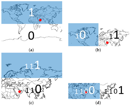
Figure 4.
Illustration of the geohash’s first coding stage. A location (the red circle) in North Africa is our reference point. Starting with the latitude axis, we can divide the global latitude interval into two parts using the equator (a). The red circle falls in the latitude interval . This region is colored in deep blue and marked as bit ’1’. The other part is dubbed ’0’. Then, in (b), the same partitioning is repeated for the longitude interval . Since the red circle is located in the deep blue area, we obtain a code of two bits ’11’ after the second division. As shown in (c,d), this is repeated until the code reaches the demanded length. All the odd bits are generated by latitude coordinates, while the even bits are generated by longitude coordinates.
2.2. Precision of the Binary Geohash
The binary geohash can infinitely subdivide the latitude and longitude space. Thus, it is capable of achieving arbitrary precision. As illustrated in Figure 4b, the first bit of the binary geohash code is 1. The red circle falls in the latitude interval . If we guess that the latitude is , then the error range of the latitude with 1 bit is . It should be noted that the error values are error bounds rather than standard deviations. Provided with more bits, the error can be dramatically reduced. As shown in Table 1, one additional bit of code can approximately halve the error. Due to the nonlinearity of the latitude and longitude coordinates, one degree of longitude at different latitudes represents different distances on the surface of the Earth. This means that a global fixed precision of the binary geohash is infeasible. We show the precision of the binary geohash around China at
N, E in Table 1. These results are estimated by an algorithm proposed for the computation of geodesics [39]. We employ a C++ implementation of the algorithm, GeodSolve [40], on the WGS-84 ellipsoid.

Table 1.
Precision of binary geohash codes with various code lengths.
2.3. Feeding Binary Geohash Codes into DNNs
Given an input feature vector , the weight vector and the nonlinear function f, a neuron of a neural network can be expressed as
Here, y is the output value, and b is the bias.
If the operation of convolution is expressed as ∗, we can rewrite Equation (1) as
Figure 5a shows the typical form of layers close to the output layer for semantic segmentation [23,25,29,41]. It implements a convolution on the feature maps from previous layers. Then, the normalized scores are obtained through the softmax layer. More specifically, Figure 6 is the architecture adopted for semantic segmentation in this paper. The output of the last upsampling layer on the bottom right of Figure 6 is in Figure 5a. The “Previous Layer” in Figure 5a is the last upsampling layer in Figure 6.
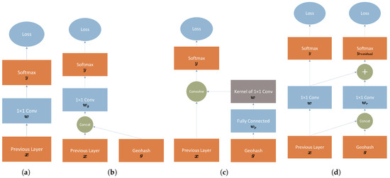
Figure 5.
Different strategies of feeding the binary geohash into neural networks: (a) a typical form of layers for semantic segmentation; (b) adding the binary geohash code to the feature space (concatenation); (c) adding the binary geohash code to the parameter space; and (d) residual correction of the output.
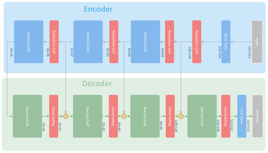
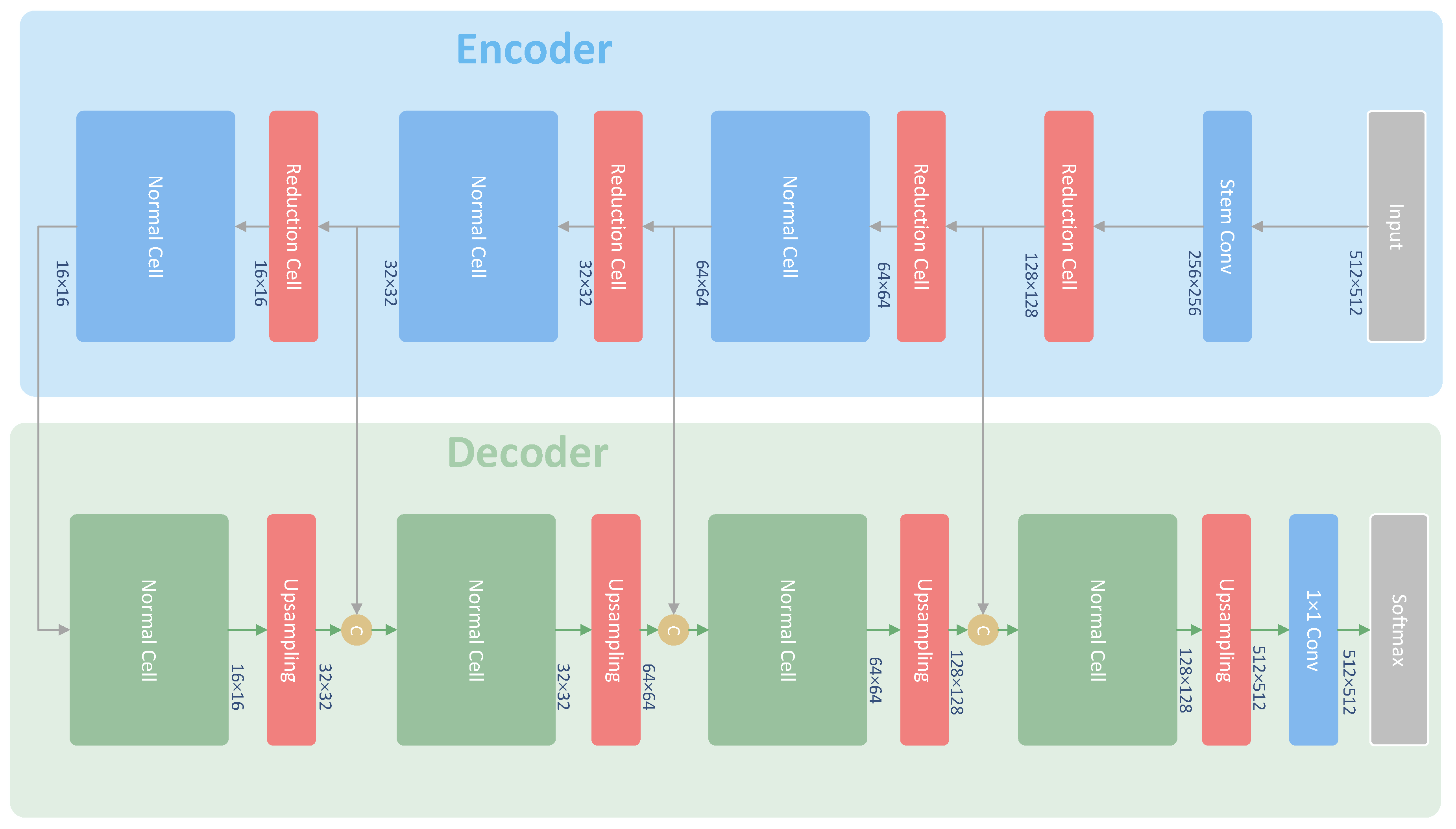
Figure 6.
The architecture of the model used for the Inria building dataset. This model, U-NASNetMobile, combines U-Net [25] with NASNet [42]. We employ Normal Cells from NASNet as the decoder part of the model. The yellow circles are concatenation layers to combine the different feature maps into a new layer.
2.3.1. Feature Space
The binary geohash code can be regarded as an additional feature. This is equivalent to transforming the original feature space into higher dimensions. Naturally, the binary geohash code can be expressed as the binary geohash vector . This method can be written as follows:
Due to the extra dimensions added by the binary geohash code, samples in this new feature space can be easier to classify.
Figure 5b shows the idea of adding the binary geohash code to CNNs. The binary geohash is first upsampled to the same size as the feature maps x from previous layers. Then, it is concatenated together with the feature maps from the previous layers along the channel axis to form a new input of a convolutional layer. This concatenation operation will increase the number of input channels before the convolutional layer. Thus, adding the binary geohash code to the feature space can be conveyed as
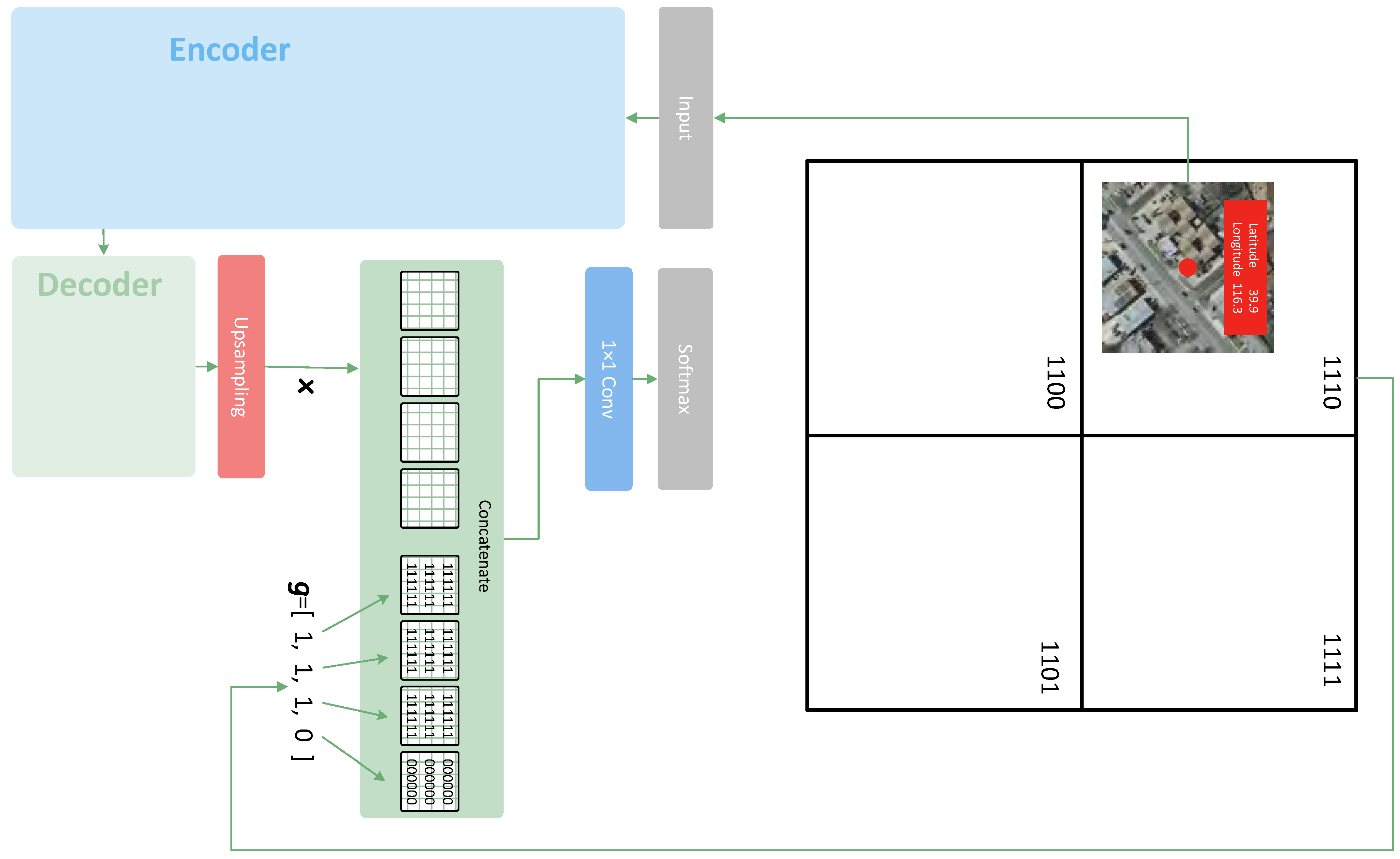
Here, is the output feature map of the previous layer. By combining Figure 6 with Figure 5b and Figure 7, we can see how this method works in practice. The “Previous Layer” in Figure 5b is the last upsampling layer in Figure 6. The geohash code vector is composed of 0 s and 1 s; for instance, in Figure 7. This vector can be resized to the size of feature map . In this example, contains four bits of code. Thus, is transformed into four channels in the form of a feature map. Then, they are combined together as the input of the convolutional layer.

Figure 7.
An example of geohash coding. First, it converts the geographic coordinates into binary bits. As shown at the top of this figure, if the center of an image tile falls into a grid, we can assign the geocode of this grid to this image. This makes the entire image tile share a common vector of the geohash code. Then, the image is fed into the convolutional neural network at the bottom. The bottom architecture is a simplified version of Figure 6, which is used for semantic segmentation. The vector of the geohash code is resized to the size of the image feature maps from the last upsampling layer of the network. Each bit corresponds to a channel of the geohash feature maps. Then, the image feature maps are concatenated with the geohash feature maps, and they form the input of the last convolutional layer together.
2.3.2. Parameter Space
Equation (1) is composed of two factors, that is, and , to accomplish the linear transformation. We can also apply the binary geohash to the parameter space. Instead of concatenating the binary geohash with the feature vector , a more aggressive method is used to replace the weight vector in Equation (1) with the weight vector learned from geohash vector :
This means that we can acquire through a fully connected layer in which the geohash vector is the input. Here, and are the linear weights and the bias of this layer, respectively. By feeding the binary geohash vector into the parameter space, this kind of strategy can control the model without touching the feature space. In this manner, the model’s parameters will be affected by the variation in the geographic coordinates. The entire function is implicitly learned from data rather than by manually configuring the model. Since the weight vector , which is the output of the linearly weighted geohash vector followed by a nonlinear transformation, is multiplied by the feature vector in Equation (7), there is a multiplicative operation before the nonlinear function. The parameters of the model increase from to , and .
Figure 5c shows the case of the convolutional neural network feeding the binary geohash vector into the parameter space. The parameters of the convolutional kernels are inferred from the binary geohash vector through a fully connected layer. Then, they are reshaped to the kernel size and convolved with the feature maps from the previous layer. For the convolution operation, Equation (7) can be rewritten as
2.3.3. Residual Correction
Residual learning has shown its power in training DNNs [43,44,45,46]. In most cases, learning targets directly from DNNs results in difficulty of convergence. Thus, residual learning is employed to mitigate this problem. In general, residual learning appears in the intermediate layers of the neural networks [43,44,45,46]. We employ a similar method, residual correction, at the end of the networks.
Figure 5d shows the key idea of residual correction. On the left branch, represents the image features extracted from the image, and is the kernel of the last convolutional layer. Thus, is the output of the last convolutional layer. After the softmax function, we can obtain the predictions of each category. For instance, the score of a pixel can be 0.95 for the building class and 0.05 for the non-building class.
On the right branch, the input of the last convolutional layer is . This means that the image features and the spatial features are combined together:
Here, is the term of residual correction, and is the output of the right head of Figure 5d. Since the softmax layer contains no parameters, the error of prediction is jointly determined by the image features and the spatial features. With the correction of the spatial features, the score of the pixel can be 0.97 for the building class and 0.03 for the non-building class. Thus, the residual correction can refine the semantic segmentation results using the binary geohash vector.
The two loss heads have the same label to learn. The left loss head is an auxiliary loss, as demonstrated in GoogLeNet [47], so we solely employ the right head for the final prediction. The left loss head only depends on the image features, and the right loss head depends on both the image features and spatial features. With the existence of the left loss, the prediction is close to 1 for the corresponding class. Thus, in Equation Equation (12), can only produce a tiny effect on the prediction of the right head.
2.3.4. Relationships in Three Approaches
In the above sections, we presented three approaches to incorporate geospatial information into neural networks. If the neural networks are expressed as , then and are the two positions used to utilize the extra spatial information. When adding the binary geohash code into the feature space, it enlarges the dimensions of . By feeding the binary geohash vector into the parameter space, it forces the weight vector to be influenced by the spatial information. Both approaches exert influences on the original positions of the neural networks. Residual correction creates a new branch to introduce the spatial information into the deep neural network without touching the original model, which merely adds a correction term to the prediction. These three approaches explore the different positions of the neural networks to employ the geospatial information.
3. Experiments
3.1. Datasets
The GID dataset [38] consists of 150 images collected from the Gaofen-2 satellite. Each image has a pixel size of and contains the R, G, and B bands. The near-infrared band is abandoned in this dataset. The spatial resolution of the multispectral image is 4 m. The GID dataset contains five land-use classes: built-up, farmland, forest, meadow and waters. We split out 90 images for training, 30 images for validation, and 30 images for testing. Each image is cropped into patches. As shown in Figure 3a, the GID dataset is uniformly distributed over China.
The Inria building dataset [6] is organized by city. There are five cities in the training set and another five cities in the test set. As shown in Figure 3b, they are distributed over the United States and Austria. Each city has 36 image tiles with a size of . We select 20 tiles from the training set for validation. The spatial resolution of the image tiles is 30 cm. This dataset contains two semantic classes: the buildings and the non-building class. Figure 2 demonstrates the statistical values of the building sizes by the number of pixels. Most of the buildings are smaller than 250,000 pixels (). Thus, we divide the image tiles into patches with a size of .
The image tiles in the GID dataset are distributed over China, and the tiles of the Inria dataset are spread over ten cities in the United States and Europe. The cover ranges of these datasets are very small to meet the requirements of real applications of semantic segmentation. Therefore, we employ a worldwide building dataset [48], called the Building dataset for Disaster Reduction and Emergency Management (DREAM-B), to approximate the real mapping situation. The image tiles are collected from Google Earth Engine (GEE) [49], and the corresponding labels are derived from Open Street Map [50]. The spatial resolution of the image tiles is 30 cm, which is quite similar to that of the Inria dataset. The size of the image tiles is . All the tiles consist of R, G, and B bands. Since the performance of the deep neural network is sensitive to the size of the training dataset, this dataset contains 626 image tiles that cover 100 worldwide cities. We split out 250 tiles for training, 63 for validation and 313 for testing.
3.2. Experimental Setup
For the GID dataset, we train a net called TernausNet, pretrained on ImageNet [51] to accelerate the convergence of training, which is based on VGG net [52] and U-net [25]. This network is referred to as the baseline. Because this dataset has the smallest size among the three datasets, we conduct experiments comparing the three ways to embed geohash codes in this dataset.
For the Inria building dataset, we conduct more experiments on this dataset by focusing on feeding the geohash into the feature space. The geohash code can solely be the input of the last convolutional layer. Furthermore, it can also be fed into the other earlier layers. As shown in Figure 6, we can also attach the geohash code after each Normal Cell. We explore both manners with various code lengths. In the end, we validate the effectiveness of feeding the geohash into the feature space on the DREAM-B dataset. The architecture of the network employed for the Inria and the DREAM-B datasets is shown in Figure 6. This model combines U-Net [25] with the NASNet-Mobile model [42], which is acquired via neural architecture searching (NAS). We refer to this model as the U-NASNetMobile, and the U-NASNetMobile model with geohash codes is termed GeohashNet ( the source code is available at https://github.com/yangnaisen/GeohashNet; accessed on 11 July 2021). The U-NASNetMobile model has a higher computation efficiency and occupies less GPU (Graphics Processing Unit) memory.
The Adam optimizer [53] is employed for training the models. Cyclic learning rates with a cosine annealing schedule [54] are utilized to accelerate the speed of convergence. This method is also referred to as cyclic cosine annealing. Based on checkpoints at the end of each cycle, snapshot ensembling [55] can further boost the accuracy of the model. The maximum and minimum learning rates of cyclic cosine annealing are and , respectively.
Data augmentations are utilized to avoid overfitting, including random flipping both horizontally and vertically, random rotation and random brightness jittering. The preprocessing of image tiles involves subtracting 128 from all the input images’ raw pixel values before dividing them by 128. The values of the geohash codes are transformed from 0 and 1 into −1 and 1, respectively. The value of weight decay is . Batch normalization [56] is set before each ReLU [57] activation layer. Models on the GID dataset are trained for 100 epochs with a mini-batch size of four. All the U-NASNetMobile experiments are trained for 200 epochs with a mini-batch size of 16. The patch size is enlarged to to further reduce the error when testing [58].
4. Results
The geospatial distribution of the Inria building dataset is very different from that of the GID dataset; it is distributed more broadly across two continents. This makes the task of semantic segmentation on this dataset more challenging. Additionally, the resolution of the Inria building dataset is much higher than that of the GID dataset, so its samples contain an enormous amount of detail. Thus, we compare three strategies of using geohash on the GID dataset and pay more attention to the Inria building dataset for visualization.
4.1. Results for the GID Dataset
The experimental results of the baseline model on the GID dataset are shown in Table 2. The results are assessed by way of the overall accuracy (OA). Upon feeding the binary geohash into the parameter space, the low accuracy indicates the dramatic influence of this method on the results of semantic segmentation. We vary the length of the binary geohash. As shown in Table 2, 14 bits result in an accuracy of , while 20 bits result in an accuracy of . This means that feeding the binary geohash into parameter space directly leads to a low accuracy regardless of the code length. Additionally, the precision of the binary geohash is a key hyperparameter for the model. All the experiments of the binary geohash show strong impacts on the results of semantic segmentation.
Table 2.
Different lengths of the binary geohash on the GID dataset.
The network of residual correction has two output nodes (shown in Figure 5d), which are highly correlated with one another. Thus, the performance of the residual correction is close to that of the baseline model. It can be seen from Table 3 that the experiment of adding the binary geohash to the feature space achieves the best performance among these methods.
Table 3.
Accuracy of the binary geohash on the GID dataset.
4.2. Results for the Inria and DREAM-B Datasets
Experiments on the Inria building dataset explore the strategy of feeding the geohash code into the feature space to further verify its effectiveness. Following the publishers of the Inria building dataset [6], we report the mean of the intersection over union (mIoU) for evaluation.
For the experiments of feeding code to the last convolutional layer, all of these groups surpass the accuracy of the baseline model, that is, , as shown in Table 4. As shown in Table 4, the geohash codes attached after each Normal Cell are lower than those of the baseline model without geohash codes. Since the length of 20 bits obtains the highest performance for both groups, the effect of code length is robust but does not vary regularly. Table 5 compares the U-NASNetMobile model with the existing methods. Table 6 provides more measurements for comparison. Though GeohashNet has a greater F1 value, it sacrifices the accuracy of precision to obtain a better recall. As shown in Figure 8a, the learning curve in the training loss keeps decreasing during training, whereas that of the validation loss stops dropping around the 75-th epoch. This suggests that there exists some degree of overfitting for models. The drastic changes of learning curves at 100 epochs are caused by the warm restarts of cyclic learning rates [54]. The U-NASNetMobile model achieves an accuracy of , which is comparable to that of the DID model’s accuracy [60] of [60], which contains fewer parameters. Since the NASNetMobile model is proposed for mobile devices, it will achieve a higher accuracy with more convolutional filters. The U-NASNetMobile model with the longitude and latitude coordinates has an accuracy of , which suggests that the longitude and latitude coordinates can also provide the geospatial information of satellite images to some extent. The longitude and latitude coordinates are expressed as the cardinal numbers, whereas the geohash codes are represented with multi-scale binary codes. Encoding the near locations with the cardinal numbers will introduce pseudo-information into the model. For instance, if three locations, A, B and C, are all at the Equator and at the longitudes of , , and , the longitudes may mislead that A is closer to B than C, because the cardinal numbers are . Due to the Earth being a spheroid, A is actually closer to C than B. The geohash codes are multi-scale binary codes without this issue. This may be the reason why the GehashNet outperforms the U-NASNetMobile model with the longitude and latitude coordinates.
Table 4.
Different lengths of the binary geohash on the Inria dataset.
Table 5.
Results for different methods on the Inria dataset.
Table 6.
More measurements of results for the Inria dataset.
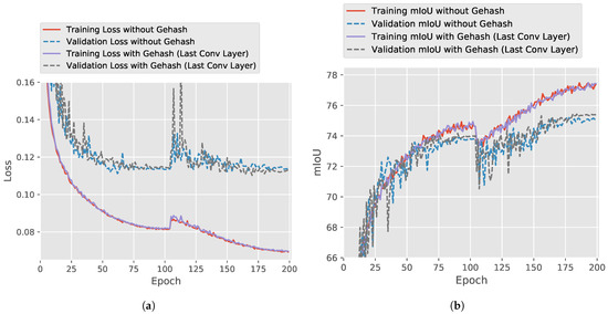
Figure 8.
Learning curves for the Inria dataset: (a) the curve of the loss; (b) the curve of mIoU.
The visual prediction results for geohash on the Inria dataset are shown in Figure 9. From the prediction of the image patches, it can be seen that most of the large buildings are recognized with small errors. The model produces rather sharp edges of the large buildings, and few small buildings fail to be correctly classified. From Figure 10, we can more clearly observe the preference of the classifier. The performance of the model may be further improved by focusing on small buildings [62,63].
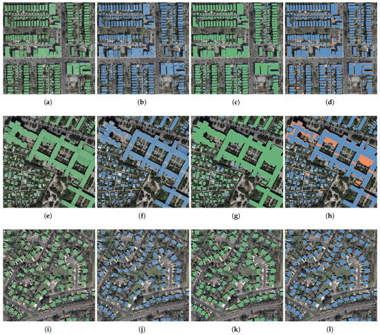
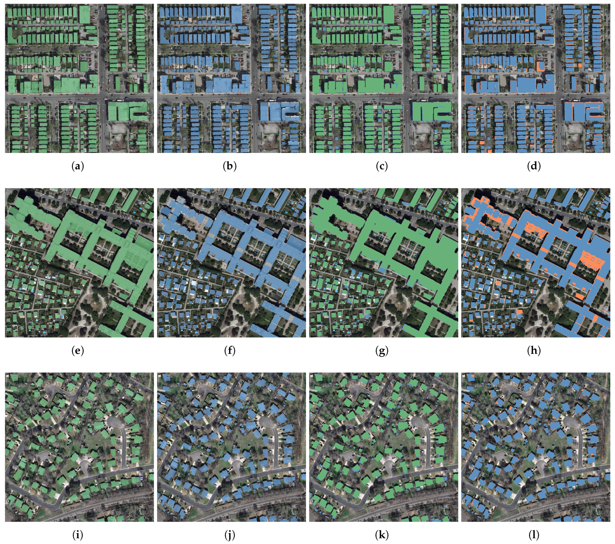
Figure 9.
Visual results for the Inria dataset. The subfigures (a,e,i) in the left column are produced by the model with the geohash. The building pixels are labeled green. The subfigures (b,f,j) in the middle column are the ground truth in a blue color, the subfigures (c,g,k) are the combination of the prediction results and the corresponding ground truth, and the subfigures (d,h,l) highlight the false positive pixels with an orange color, which are misclassified as buildings. All the sample images have a size of .
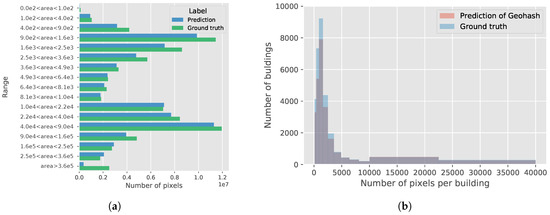
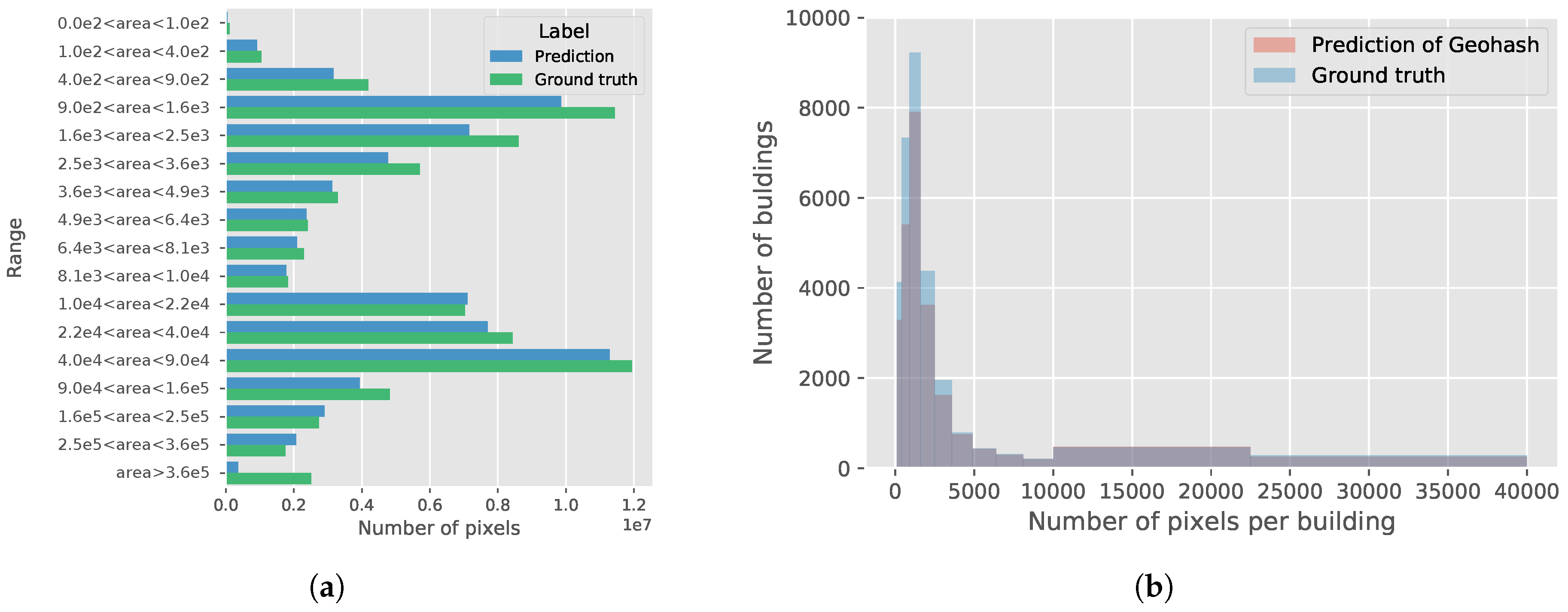
Figure 10.
Comparison of the model predictions and the ground truth on the validation set of the Inria building dataset: (a) the area of the building size is used as the indicator for comparison; (b) the number of buildings is used as the indicator for comparison. From the figures, it can be clearly seen that small buildings fail to be correctly classified in terms of area and number of buildings. It should be noted that the intervals of building size in both figures are not divided evenly.
The experiments on the DREAM-B dataset further validate the effectiveness of geohash codes. As shown in Table 7, the model with a geohash code of 16 bits surpasses the baseline model without geohash codes by . As with the results for the Inria dataset, models with various code lengths trained on the DREAM-B dataset perform better than the baseline model.
Table 7.
Different lengths of the binary geohash on the DREAM-B dataset.
5. Discussion
5.1. The Influence of Code Length
In Table 4, the length of 20 bits achieves the best result, that is, , which outperforms the baseline model with a margin of . With various lengths of code, the accuracy of the model varies in the interval . This suggests that the length of geohash codes has a considerable influence on the model.
The geographic hash codes can enhance the spatial information. However, this kind of enhancement may cause overfitting of the model. If the spatial information is too strong, the neural networks will just learn the correlation between the geographic position and the corresponding labels. This indeed causes the overfitting of the model. To avoid this situation, the model should learn mainly from image features rather than from geospatial features. The geospatial features are the only assistance for the input images. Therefore, we can use the precision of the geohash codes to prevent the dominance of geospatial features in semantic segmentation.
5.2. Ablation Study and Visualization
To thoroughly investigate how the binary geohash code affects the model, we analyze the prediction results both quantitatively and qualitatively. Table 8 presents the confusion matrices of the two models, both with and without geohash codes, trained on the Inria dataset. From Table 8, it can be seen that pixels of the non-building class dominate the dataset, with a proportion of % in total, and the building class has a percentage of %. Comparing the number of predicted pixels of the non-building class, the model with geohash codes tends to classify fewer pixels in the non-building class. The normalized confusion matrices normalizing the elements in each row illustrate this trend more clearly. The model with geohash codes correctly predicts % of the building pixels. This result is better than that of the model without geohash codes (%). The prediction results for the non-building class of both models are roughly equal.
Table 8.
Confusion matrices of models with and without geohash codes trained on the Inria dataset. Normalized confusion matrix normalizes the elements in each row.
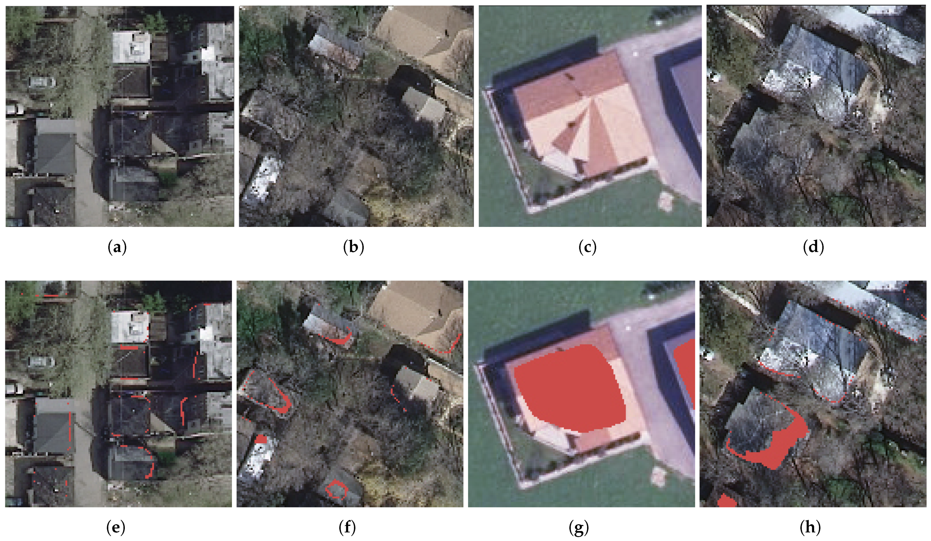
The overall influence of the geohash codes can be clearly observed in Figure 11. For the model with geohash codes attached, a sensitivity analysis can help us to better understand how the geohash codes affect the results. This is accomplished by setting the geohash code to all zeros to eliminate its impact. After zeroing the geohash code, the pixels affected by the spatial distribution altered predictions in the semantic segmentation. Samples of the altered area are illustrated in Figure 11. In the subfigures of (e,f,h), the majority of the altered pixels appear on the border of the buildings, while some regions of the buildings are radically changed in the the subfigure (g).

Figure 11.
Impacts of the binary geohash. By setting the geohash code to zeros, the impacts of the geospatial information are thoroughly eliminated. After zeroing the geohash codes, the changed labels are marked in a red color. Subfigures of (a–d) are samples from the Inria dataset. In the subfigures of (e,f,h), the majority of the altered pixels appear on the border of buildings, while some regions of the buildings are radically changed in the subfigure (g). All the sample images have a size of .
The purpose of adding geohash codes to the model is to make the model obtain helpful information from the geographic location of the image. From Figure 9, which depicts the semantic segmentation results, we can see that when the geographic location information is not considered, the neural network can identify the main body of the buildings according to the characteristics of the image itself. The majority of the semantic segmentation results within the building are correct, and most of the pixels with wrong labels occur on the edge of the building. The pixels within the buildings have been classified correctly, thus it can be recognized without the need for geographic location information. Adding geographic location information will not change the pixels that have been classified correctly in the buildings. Therefore, the pixels that change category appear on the edge of the building after adding the geohash codes.
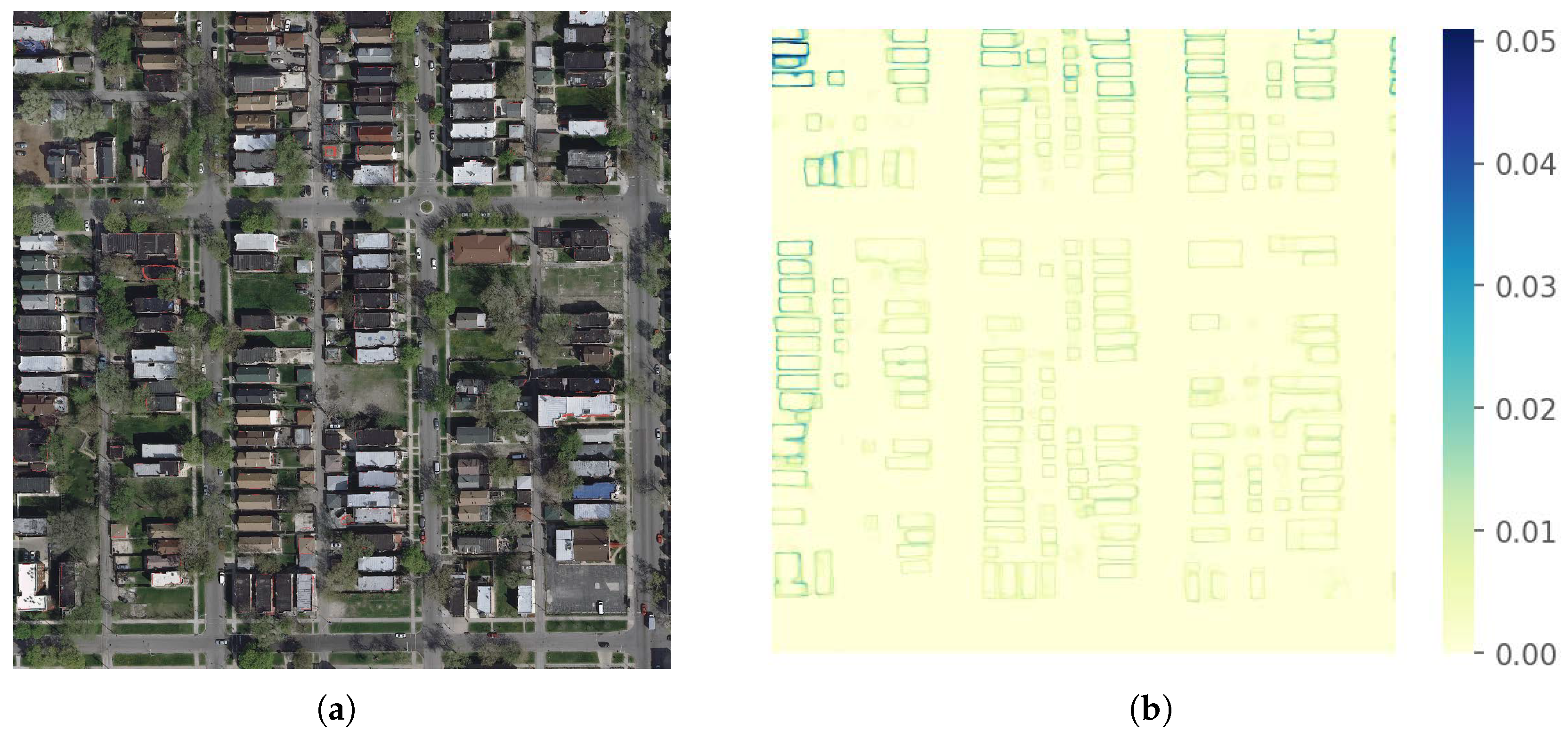
The heat map in Figure 12 can isolate this kind of variation. The prediction scores of the buildings influenced by geohash codes fluctuate from 0 to . For small buildings, a greater portion of the building area is affected. The visualization results for the geohash codes verify the strong impact of the geospatial information on the semantic segmentation results. Thus, they confirm the effectiveness of the proposed binary geohash method.

Figure 12.
The impacts of the binary geohash can be better recognized by a heat map of the buildings’ prediction score. The buildings’ prediction scores are the output of the softmax layer within the range . The heat map is obtained by visualizing the absolute values of the difference between the prediction scores of the geohash codes and the zeroed codes. The sample images have a size of .
6. Conclusions
Satellite images have shown strong spatial patterns in a great many applications and datasets. Adapting the model according to the geospatial location of data is the missing part of the traditional deep learning approaches. In this paper, we studied the approach of integrating geospatial information into DNNs based on the geohash method. Specifically, a binary geohash code with bits of 0 and 1 was utilized in the proposed method. We conducted three strategies to combine the binary geohash code with the existing architectures of CNNs: feature space, parameter space, and residual correction. Experiments were conducted on three widely distributed datasets to investigate the best manner of using the geographic coordinates. The results for the experiments demonstrate that the simplest approach of treating the binary geohash code as an extra feature map is the most effective method. Additionally, the impact of the precision of the binary geohash code was analyzed in detail. All of these results demonstrate that the geospatial information has a non-negligible influence on the large-scale semantic segmentation of satellite images, and the proposed method can, to some extent, learn this type of geospatial information.
This paper is an attempt to utilize the spatial information of remote sensing data. Geospatial locations are regarded as part of the input data. Another possible way is to transform the spatial information into the component of the model rather than the component of the data, which has not been explored in this paper. In a larger sense, extracting knowledge from remote sensing data is not touched on in this research and is still a big challenge worth studying. Besides, the currently employed dataset contains only a few categories. In the future, we will investigate the different impacts of geospatial information on specific land-use classes using more datasets.
Author Contributions
Conceptualization, formal analysis, H.T. and N.Y.; methodology, software, validation, investigation, resources, data curation, writing—original draft preparation, visualization, N.Y.; writing—review and editing, supervision, project administration, funding acquisition, H.T. All authors have read and agreed to the published version of the manuscript.
Funding
This work was supported in part by the National Natural Science Foundation of China under Grant 41971280 and in part by the National Key R&D Program of China under Grant 2017YFB0504104.
Data Availability Statement
Publicly available datasets were analyzed in this study. These datasets can be found here: https://x-ytong.github.io/project/GID.html and https://project.inria.fr/aerialimagelabeling/; accessed on 11 July 2021.
Acknowledgments
We would like to thank the high-performance computing support from the Center for Geodata and Analysis, Faculty of Geographical Science, Beijing Normal University [https://gda.bnu.edu.cn/; accessed on 11 July 2021].
Conflicts of Interest
The authors declare no conflict of interest. The funders had no role in the design of the study; in the collection, analyses, or interpretation of data; in the writing of the manuscript, or in the decision to publish the results.
Abbreviations
The following abbreviations are used in this manuscript:
| ASPP | Atrous Spatial Pyramid Pooling |
| BN | Batch Normalization |
| CNNs | Convolutional Neural Networks |
| DID | Dense In Dense |
| DNNs | Deep Neural Networks |
| DREAM-B | Building dataset for Disaster Reduction and Emergence Management |
| FCN | Fully Convolutional Network |
| GEE | Google Earth Engine |
| GID | Gaofen Image Dataset |
| GPU | Graphics Processing Unit |
| mIoU | mean of Intersection over Union |
| NAS | Neural Architecture Searching |
| OA | Overall Accuracy |
| PSPNet | Pyramid Scene Parsing Network |
| ReLU | Rectified Linear Unit |
References
- Tobler, W.R. A computer movie simulating urban growth in the Detroit region. Econ. Geogr. 1970, 46, 234–240. [Google Scholar] [CrossRef]
- Liu, X.; Hu, G.; Chen, Y.; Li, X.; Xu, X.; Li, S.; Pei, F.; Wang, S. High-resolution multi-temporal mapping of global urban land using Landsat images based on the Google Earth Engine Platform. Remote Sens. Environ. 2018, 209, 227–239. [Google Scholar] [CrossRef]
- Schneider, A.; Friedl, M.A.; Potere, D. Mapping global urban areas using MODIS 500-m data: New methods and datasets based on ‘urban ecoregions’. Remote Sens. Environ. 2010, 114, 1733–1746. [Google Scholar] [CrossRef]
- Zhang, H.K.; Roy, D.P. Using the 500 m MODIS land cover product to derive a consistent continental scale 30 m Landsat land cover classification. Remote Sens. Environ. 2017, 197, 15–34. [Google Scholar] [CrossRef]
- Chen, J.; Chen, J.; Liao, A.; Cao, X.; Chen, L.; Chen, X.; He, C.; Han, G.; Peng, S.; Lu, M.; et al. Global land cover mapping at 30 m resolution: A POK-based operational approach. ISPRS J. Photogramm. Remote. Sens. 2015, 103, 7–27. [Google Scholar] [CrossRef] [Green Version]
- Maggiori, E.; Tarabalka, Y.; Charpiat, G.; Alliez, P. Can semantic labeling methods generalize to any city? the inria aerial image labeling benchmark. In Proceedings of the IEEE International Geoscience and Remote Sensing Symposium (IGARSS), Fort Worth, TX, USA, 23–28 July 2017; pp. 3226–3229. [Google Scholar]
- Pesaresi, M.; Huadong, G.; Blaes, X.; Ehrlich, D.; Ferri, S.; Gueguen, L.; Halkia, M.; Kauffmann, M.; Kemper, T.; Lu, L.; et al. A global human settlement layer from optical HR/VHR RS data: Concept and first results. IEEE J. Sel. Top. Appl. Earth Obs. Remote Sens. 2013, 6, 2102–2131. [Google Scholar] [CrossRef]
- Lu, K.; Sun, Y.; Ong, S.H. Dual-Resolution U-Net: Building Extraction from Aerial Images. In Proceedings of the 24th International Conference on Pattern Recognition (ICPR), Beijing, China, 20–24 August 2018; pp. 489–494. [Google Scholar]
- Neimeyer, G. Geohash, 2008. Available online: http://geohash.org (accessed on 11 July 2021).
- Balkić, Z.; Šoštarić, D.; Horvat, G. GeoHash and UUID identifier for multi-agent systems. In KES International Symposium on Agent and Multi-Agent Systems: Technologies and Applications, Proceedings of the 6th KES International Conference, KES-AMSTA 2012, Dubrovnik, Croatia, 25–27 June 2012; Springer: Berlin/Heidelberg, Germany, 2012; pp. 290–298. [Google Scholar]
- Fox, A.; Eichelberger, C.; Hughes, J.; Lyon, S. Spatio-temporal indexing in non-relational distributed databases. In Proceedings of the IEEE International Conference on Big Data, Silicon Valley, CA, USA, 6–9 October 2013; pp. 291–299. [Google Scholar]
- Liu, J.; Li, H.; Gao, Y.; Yu, H.; Jiang, D. A geohash-based index for spatial data management in distributed memory. In Proceedings of the 22nd International Conference on Geoinformatics, Kaohsiung, Taiwan, 25–27 June 2014; pp. 1–4. [Google Scholar]
- Suwardi, I.S.; Dharma, D.; Satya, D.P.; Lestari, D.P. Geohash index based spatial data model for corporate. In Proceedings of the International Conference on Electrical Engineering and Informatics (ICEEI), Denpasar, Indonesia, 10–11 August 2015; pp. 478–483. [Google Scholar]
- Tang, K.D.; Paluri, M.; Fei-Fei, L.; Fergus, R.; Bourdev, L.D. Improving Image Classification with Location Context. In Proceedings of the 2015 IEEE International Conference on Computer Vision (ICCV), Santiago, Chile, 7–13 December 2015; pp. 1008–1016. [Google Scholar]
- Rahimi, A.; Baldwin, T.; Cohn, T. Continuous Representation of Location for Geolocation and Lexical Dialectology using Mixture Density Networks. arXiv 2017, arXiv:1708.04358. [Google Scholar]
- Yang, L.; Cervone, G. Analysis of remote sensing imagery for disaster assessment using deep learning: A case study of flooding event. Soft Comput. 2019, 23, 13393–13408. [Google Scholar] [CrossRef]
- Ohlander, R.; Price, K.; Reddy, D. Picture segmentation using a recursive region splitting method. Comput. Graph. Image Process. 1978, 8, 313–333. [Google Scholar] [CrossRef]
- Geman, S.; Geman, D. Stochastic Relaxation, Gibbs Distributions, and the Bayesian Restoration of Images. IEEE Trans. Pattern Anal. Mach. Intell. 1984, PAMI-6, 721–741. [Google Scholar] [CrossRef]
- Shi, J.; Malik, J. Normalized cuts and image segmentation. IEEE Trans. Pattern Anal. Mach. Intell. 2000, 22, 888–905. [Google Scholar]
- Belongie, S.J.; Carson, C.; Greenspan, H.; Malik, J. Color- and texture-based image segmentation using EM and its application to content-based image retrieval. In Proceedings of the Sixth International Conference on Computer Vision (IEEE Cat. No.98CH36271), Bombay, India, 7 January 1998; pp. 675–682. [Google Scholar]
- Lafferty, J.; McCallum, A.; Pereira, F. Conditional random fields: Probabilistic models for segmenting and labeling sequence data. In Proceedings of the Eighteenth International Conference on Machine Learning, ICML, Williamstown, MA, USA, 28 June 2001; Volume 1, pp. 282–289. [Google Scholar]
- Mobahi, H.; Rao, S.R.; Yang, A.; Sastry, S.; Ma, Y. Segmentation of Natural Images by Texture and Boundary Compression. Int. J. Comput. Vis. 2011, 95, 86–98. [Google Scholar] [CrossRef] [Green Version]
- Long, J.; Shelhamer, E.; Darrell, T. Fully convolutional networks for semantic segmentation. In Proceedings of the IEEE Conference on Computer Vision and Pattern Recognition, Santiago, Chile, 7–13 December 2015; pp. 3431–3440. [Google Scholar]
- Noh, H.; Hong, S.; Han, B. Learning deconvolution network for semantic segmentation. In Proceedings of the IEEE International Conference on Computer Vision, Santiago, Chile, 7–13 December 2015; pp. 1520–1528. [Google Scholar]
- Ronneberger, O.; Fischer, P.; Brox, T. U-net: Convolutional networks for biomedical image segmentation. In International Conference on Medical Image Computing and Computer-Assisted Intervention, Proceedings of the 18th International Conference, Munich, Germany, 5–9 October 2015; Springer: Berlin/Heidelberg, Germany, 2015; pp. 234–241. [Google Scholar]
- Yu, F.; Koltun, V. Multi-scale context aggregation by dilated convolutions. arXiv 2015, arXiv:1511.07122. [Google Scholar]
- Chen, L.C.; Papandreou, G.; Kokkinos, I.; Murphy, K.; Yuille, A.L. Deeplab: Semantic image segmentation with deep convolutional nets, atrous convolution, and fully connected crfs. IEEE Trans. Pattern Anal. Mach. Intell. 2017, 40, 834–848. [Google Scholar] [CrossRef] [PubMed]
- Chen, L.C.; Papandreou, G.; Schroff, F.; Adam, H. Rethinking atrous convolution for semantic image segmentation. arXiv 2017, arXiv:1706.05587. [Google Scholar]
- Zhao, H.; Shi, J.; Qi, X.; Wang, X.; Jia, J. Pyramid scene parsing network. In Proceedings of the IEEE Conference on Computer Vision and Pattern Recognition, Honolulu, HI, USA, 21–26 July 2017; pp. 2881–2890. [Google Scholar]
- Mnih, V. Machine Learning for Aerial Image Labeling; Citeseer, 2013. Available online: http://www.cs.toronto.edu/~vmnih/docs (accessed on 11 July 2021).
- Yuan, J. Learning building extraction in aerial scenes with convolutional networks. IEEE Trans. Pattern Anal. Mach. Intell. 2017, 40, 2793–2798. [Google Scholar] [CrossRef]
- Huang, B.; Lu, K.; Audeberr, N.; Khalel, A.; Tarabalka, Y.; Malof, J.; Boulch, A.; Le Saux, B.; Collins, L.; Bradbury, K.; et al. Large-scale semantic classification: Outcome of the first year of inria aerial image labeling benchmark. In Proceedings of the IGARSS 2018-2018 IEEE International Geoscience and Remote Sensing Symposium, Valencia, Spain, 22–27 July 2018; pp. 6947–6950. [Google Scholar]
- Yang, H.L.; Yuan, J.; Lunga, D.; Laverdiere, M.; Rose, A.; Bhaduri, B. Building extraction at scale using convolutional neural network: Mapping of the united states. IEEE J. Sel. Top. Appl. Earth Obs. Remote Sens. 2018, 11, 2600–2614. [Google Scholar] [CrossRef] [Green Version]
- Xia, G.S.; Hu, J.; Hu, F.; Shi, B.; Bai, X.; Zhong, Y.; Zhang, L.; Lu, X. AID: A benchmark dataset for performance evaluation of aerial scene classification. IEEE Trans. Geosci. Remote Sens. 2017, 55, 3965–3981. [Google Scholar] [CrossRef] [Green Version]
- Cheng, G.; Han, J.; Lu, X. Remote sensing image scene classification: Benchmark and state of the art. Proc. IEEE 2017, 105, 1865–1883. [Google Scholar] [CrossRef] [Green Version]
- ISPRS 2D Semantic Labeling Benchmark.
- Xia, G.S.; Bai, X.; Ding, J.; Zhu, Z.; Belongie, S.; Luo, J.; Datcu, M.; Pelillo, M.; Zhang, L. DOTA: A large-scale dataset for object detection in aerial images. In Proceedings of the IEEE Conference on Computer Vision and Pattern Recognition (CVPR), Salt Lake City, UT, USA, 18–23 June 2018. [Google Scholar]
- Tong, X.Y.; Xia, G.S.; Lu, Q.; Shen, H.; Li, S.; You, S.; Zhang, L. Learning Transferable Deep Models for Land-Use Classification with High-Resolution Remote Sensing Images. arXiv 2018, arXiv:1807.05713. [Google Scholar]
- Karney, C.F. Algorithms for geodesics. J. Geod. 2013, 87, 43–55. [Google Scholar] [CrossRef] [Green Version]
- Karney, C. GeographicLib, 2016. Available online: https://sourceforge.net/projects/geographiclib/ (accessed on 11 July 2021).
- Badrinarayanan, V.; Kendall, A.; Cipolla, R. Segnet: A deep convolutional encoder-decoder architecture for image segmentation. IEEE Trans. Pattern Anal. Mach. Intell. 2017, 39, 2481–2495. [Google Scholar] [CrossRef] [PubMed]
- Zoph, B.; Vasudevan, V.; Shlens, J.; Le, Q.V. Learning transferable architectures for scalable image recognition. In Proceedings of the IEEE Conference on Computer Vision and Pattern Recognition, Salt Lake City, UT, USA, 18–23 June 2018; pp. 8697–8710. [Google Scholar]
- He, K.; Zhang, X.; Ren, S.; Sun, J. Deep residual learning for image recognition. In Proceedings of the IEEE Conference on Computer Vision and Pattern Recognition, Las Vegas, NV, USA, 27–30 June 2016; pp. 770–778. [Google Scholar]
- Xie, S.; Girshick, R.; Dollár, P.; Tu, Z.; He, K. Aggregated residual transformations for deep neural networks. In Proceedings of the IEEE Conference on Computer Vision and Pattern Recognition, Honolulu, HI, USA, 21–26 July 2017; pp. 1492–1500. [Google Scholar]
- Szegedy, C.; Ioffe, S.; Vanhoucke, V.; Alemi, A.A. Inception-v4, inception-resnet and the impact of residual connections on learning. In Proceedings of the Thirty-First AAAI Conference on Artificial Intelligence, San Francisco, CA, USA, 4–9 February 2017. [Google Scholar]
- Hu, J.; Shen, L.; Sun, G. Squeeze-and-excitation networks. In Proceedings of the IEEE Conference on Computer Vision and Pattern Recognition, Salt Lake City, UT, USA, 18–23 June 2018; pp. 7132–7141. [Google Scholar]
- Szegedy, C.; Liu, W.; Jia, Y.; Sermanet, P.; Reed, S.; Anguelov, D.; Erhan, D.; Vanhoucke, V.; Rabinovich, A. Going deeper with convolutions. In Proceedings of the IEEE Conference on Computer Vision and Pattern Recognition, Santiago, Chile, 7–13 December 2015; pp. 1–9. [Google Scholar]
- Yang, N.; Tang, H. GeoBoost: An Incremental Deep Learning Approach toward Global Mapping of Buildings from VHR Remote Sensing Images. Remote Sens. 2020, 12, 1794. [Google Scholar] [CrossRef]
- Gorelick, N.; Hancher, M.; Dixon, M.; Ilyushchenko, S.; Thau, D.; Moore, R. Google Earth Engine: Planetary-scale geospatial analysis for everyone. Remote Sens. Environ. 2017, 202, 18–27. [Google Scholar] [CrossRef]
- Haklay, M.; Weber, P. Openstreetmap: User-generated street maps. IEEE Pervasive Comput. 2008, 7, 12–18. [Google Scholar] [CrossRef] [Green Version]
- Iglovikov, V.; Shvets, A. TernausNet: U-Net with VGG11 Encoder Pre-Trained on ImageNet for Image Segmentation. arXiv 2018, arXiv:1801.05746. [Google Scholar]
- Simonyan, K.; Zisserman, A. Very deep convolutional networks for large-scale image recognition. arXiv 2014, arXiv:1409.1556. [Google Scholar]
- Kingma, D.; Ba, J. Adam: A method for stochastic optimization. arXiv 2014, arXiv:1412.6980. [Google Scholar]
- Loshchilov, I.; Hutter, F. Sgdr: Stochastic gradient descent with warm restarts. arXiv 2016, arXiv:1608.03983. [Google Scholar]
- Huang, G.; Li, Y.; Pleiss, G.; Liu, Z.; Hopcroft, J.E.; Weinberger, K.Q. Snapshot ensembles: Train 1, get m for free. arXiv 2017, arXiv:1704.00109. [Google Scholar]
- Ioffe, S.; Szegedy, C. Batch normalization: Accelerating deep network training by reducing internal covariate shift. In Proceedings of the International Conference on Machine Learning, Lille, France, 6–11 July 2015; pp. 448–456. [Google Scholar]
- Nair, V.; Hinton, G.E. Rectified linear units improve restricted boltzmann machines. In Proceedings of the 27th International Conference on Machine Learning (ICML-10), Haifa, Israel, 21–24 June 2010; pp. 807–814. [Google Scholar]
- Huang, B.; Collins, L.M.; Bradbury, K.; Malof, J.M. Deep Convolutional Segmentation of Remote Sensing Imagery: A Simple and Efficient Alternative to Stitching Output Labels. In Proceedings of the IGARSS 2018-2018 IEEE International Geoscience and Remote Sensing Symposium, Valencia, Spain, 22–27 July 2018; pp. 6899–6902. [Google Scholar]
- He, C.; Fang, P.; Zhang, Z.; Xiong, D.; Liao, M. An End-to-End Conditional Random Fields and Skip-Connected Generative Adversarial Segmentation Network for Remote Sensing Images. Remote Sens. 2019, 11, 1604. [Google Scholar] [CrossRef] [Green Version]
- Hu, T. Dense In Dense: Training Segmentation from Scratch. In Asian Conference on Computer Vision, Proceedings of the 14th Asian Conference on Computer Vision, Perth, Australia, 2–6 December 2018; Springer: Berlin/Heidelberg, Germany, 2018; pp. 454–470. [Google Scholar]
- Chatterjee, B.; Poullis, C. On Building Classification from Remote Sensor Imagery Using Deep Neural Networks and the Relation Between Classification and Reconstruction Accuracy Using Border Localization as Proxy. In Proceedings of the 16th Conference on Computer and Robot Vision (CRV), Kingston, QC, Canada, 29–31 May 2019; pp. 41–48. [Google Scholar]
- Kampffmeyer, M.; Salberg, A.B.; Jenssen, R. Semantic segmentation of small objects and modeling of uncertainty in urban remote sensing images using deep convolutional neural networks. In Proceedings of the IEEE Conference on Computer Vision and Pattern Recognition Workshops, Las Vegas, NV, USA, 27–30 June 2016; pp. 1–9. [Google Scholar]
- Hu, P.; Ramanan, D. Finding tiny faces. In Proceedings of the IEEE Conference on Computer Vision and Pattern Recognition, Honolulu, HI, USA, 21–26 July 2017; pp. 951–959. [Google Scholar]


Publisher’s Note: MDPI stays neutral with regard to jurisdictional claims in published maps and institutional affiliations. |
© 2021 by the authors. Licensee MDPI, Basel, Switzerland. This article is an open access article distributed under the terms and conditions of the Creative Commons Attribution (CC BY) license (https://creativecommons.org/licenses/by/4.0/).