
Deep Learning on Airborne Radar Echograms for Tracing Snow Accumulation Layers of the Greenland Ice Sheet

 , , ,
, , ,  , and
, and
Abstract
:
1. Introduction
2. Related Work
2.1. Ice Layer Tracking Techniques
2.1.1. Ice Surface and Bottom Detection
2.1.2. Internal Ice Layer Detection
2.2. Fully Convolutional Networks
3. Dataset
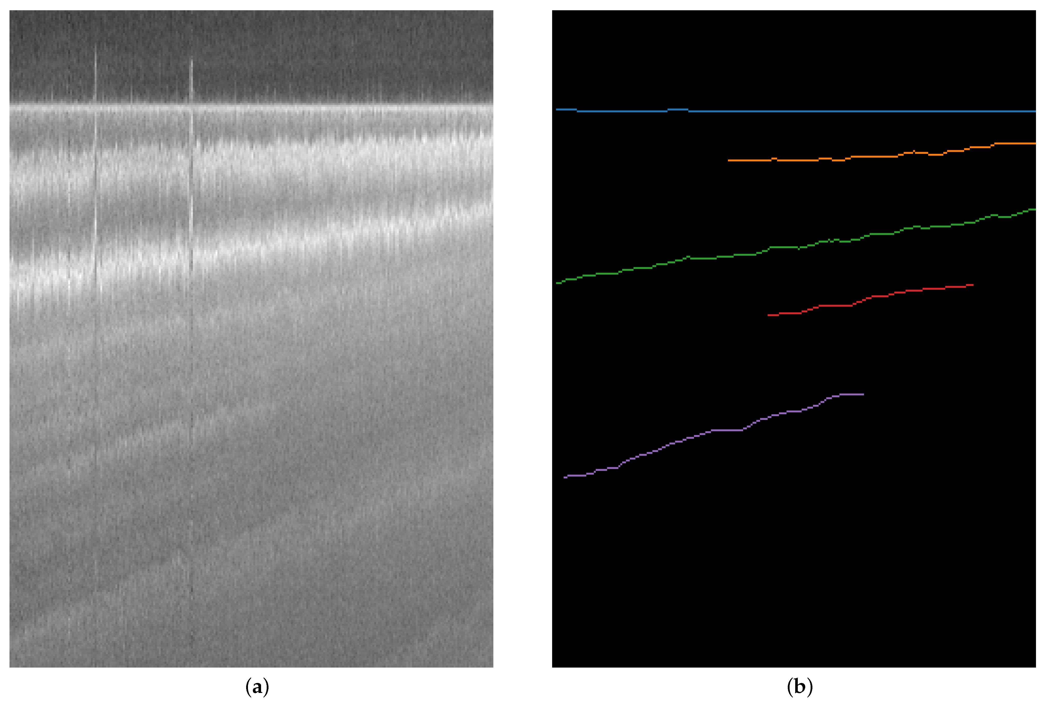
3.1. Characteristics
3.2. Challenges
4. Methodology
4.1. Pre-Processing
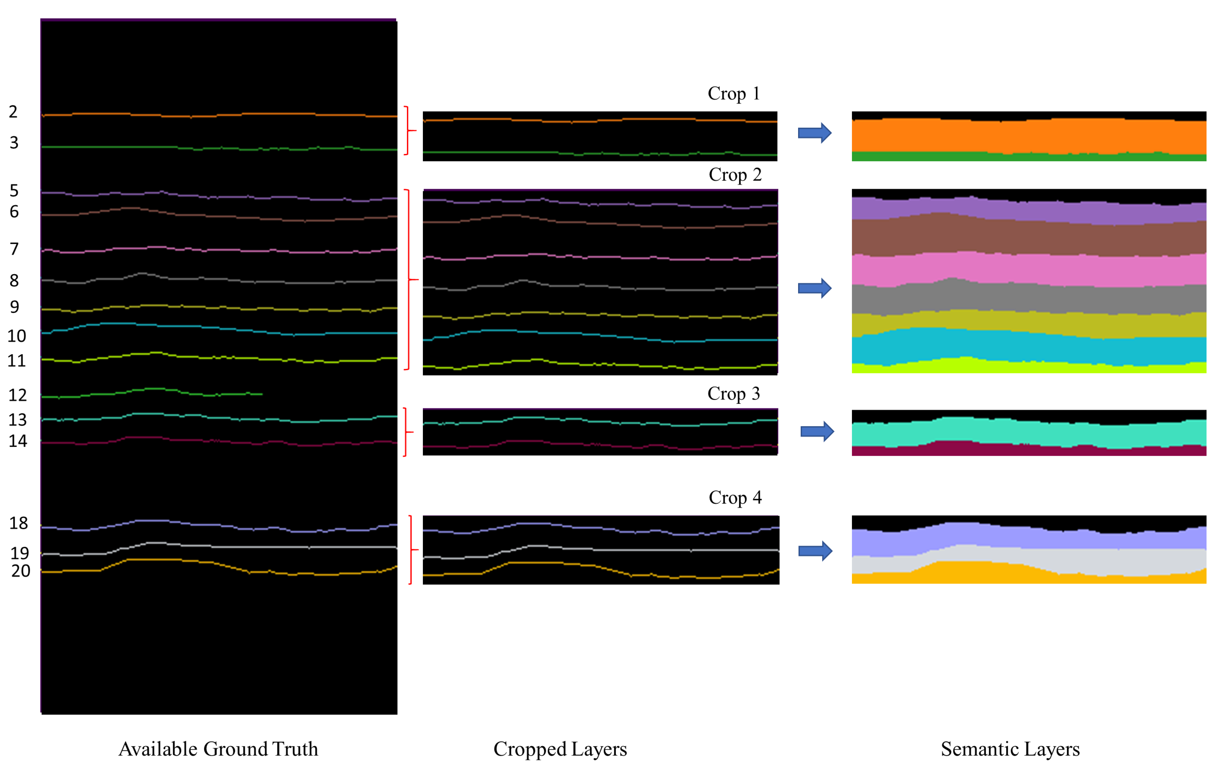
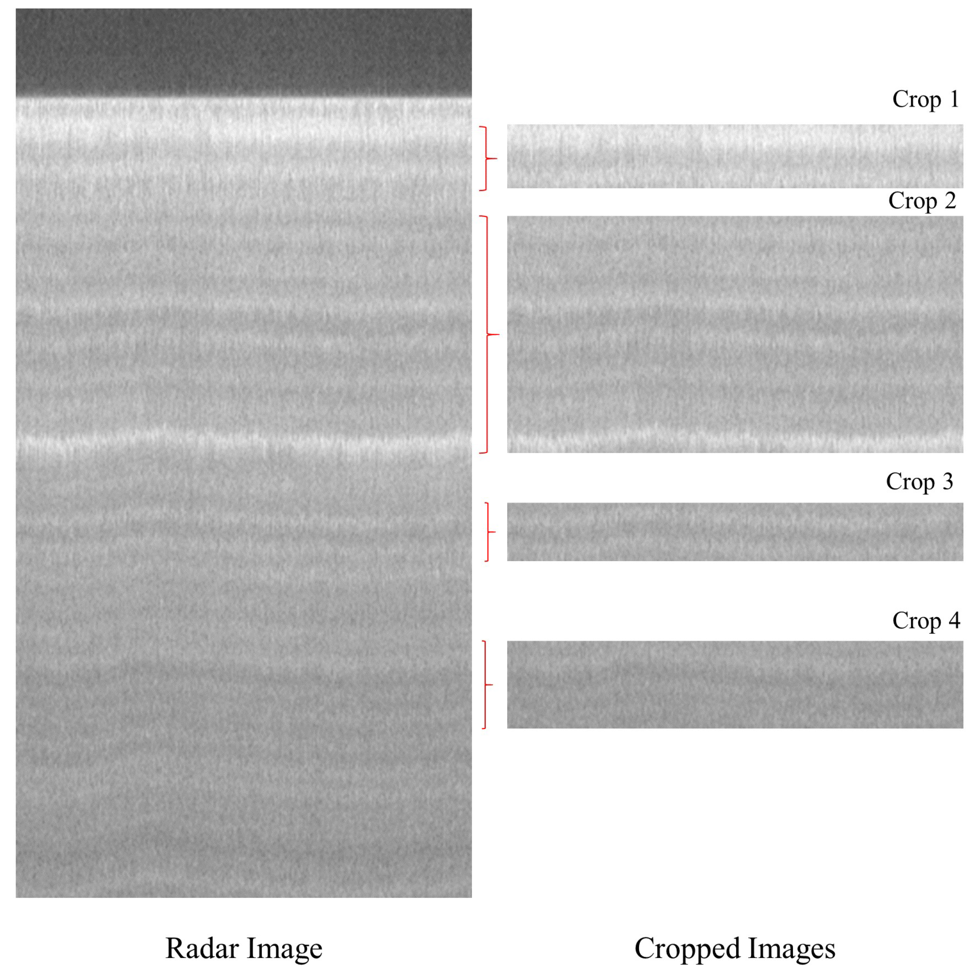
4.1.1. Image Cropping
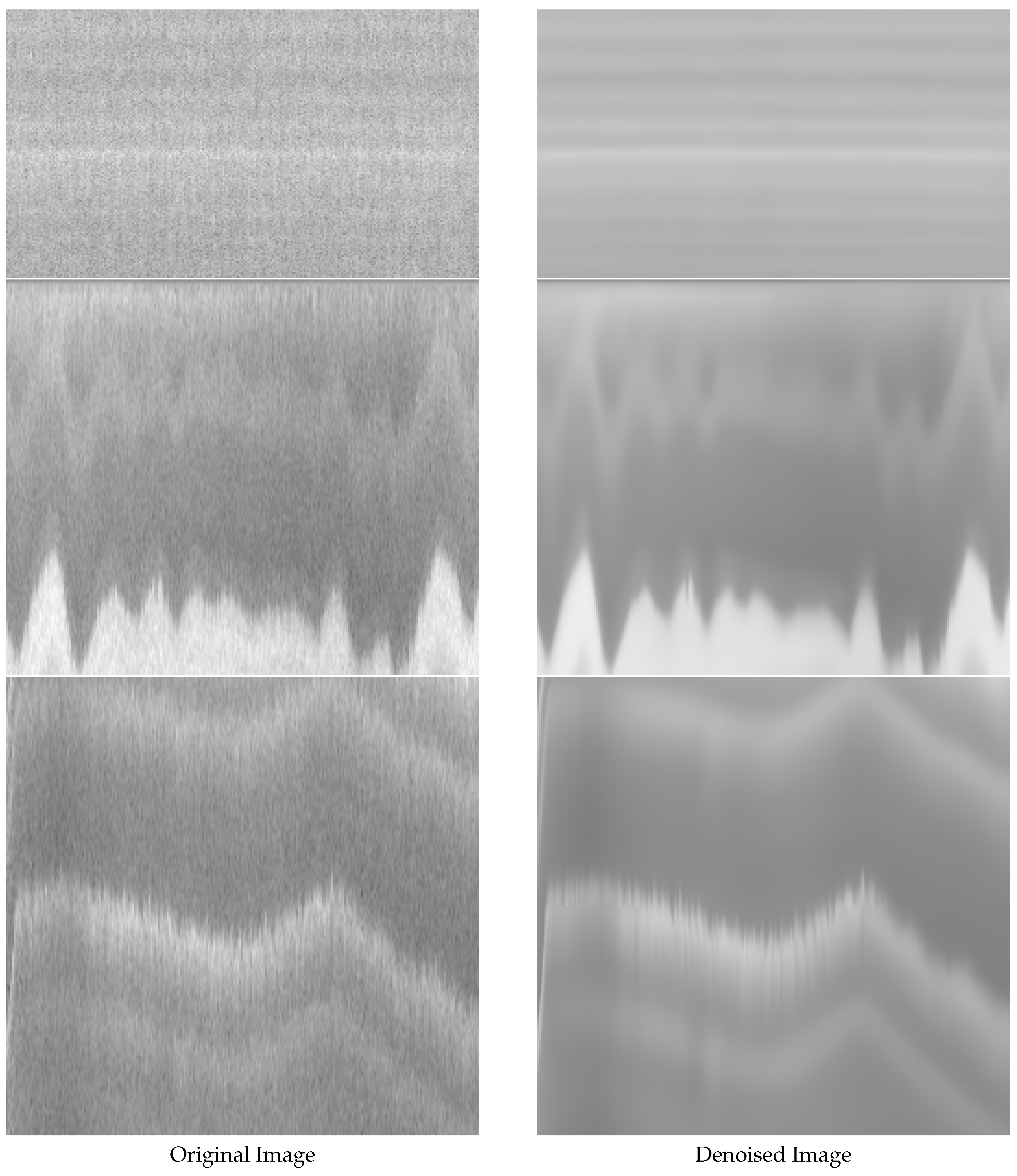
4.1.2. Denoising
4.2. FCN Architectures
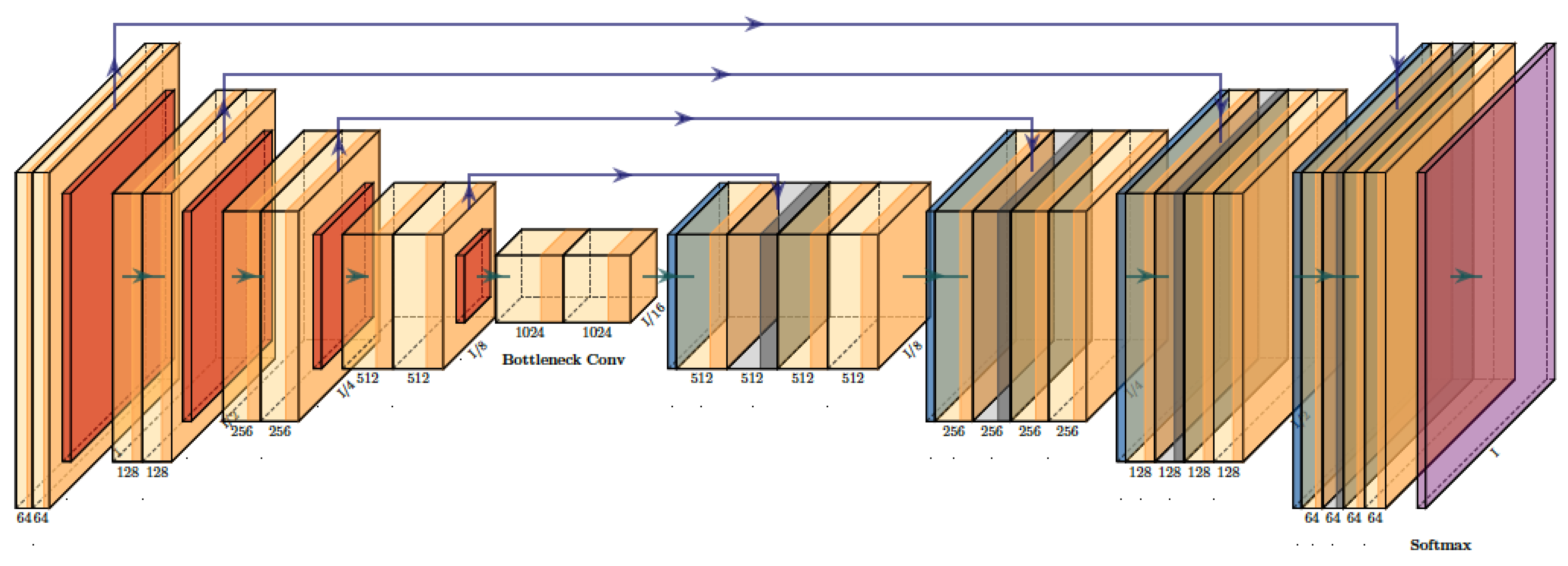
4.2.1. UNet
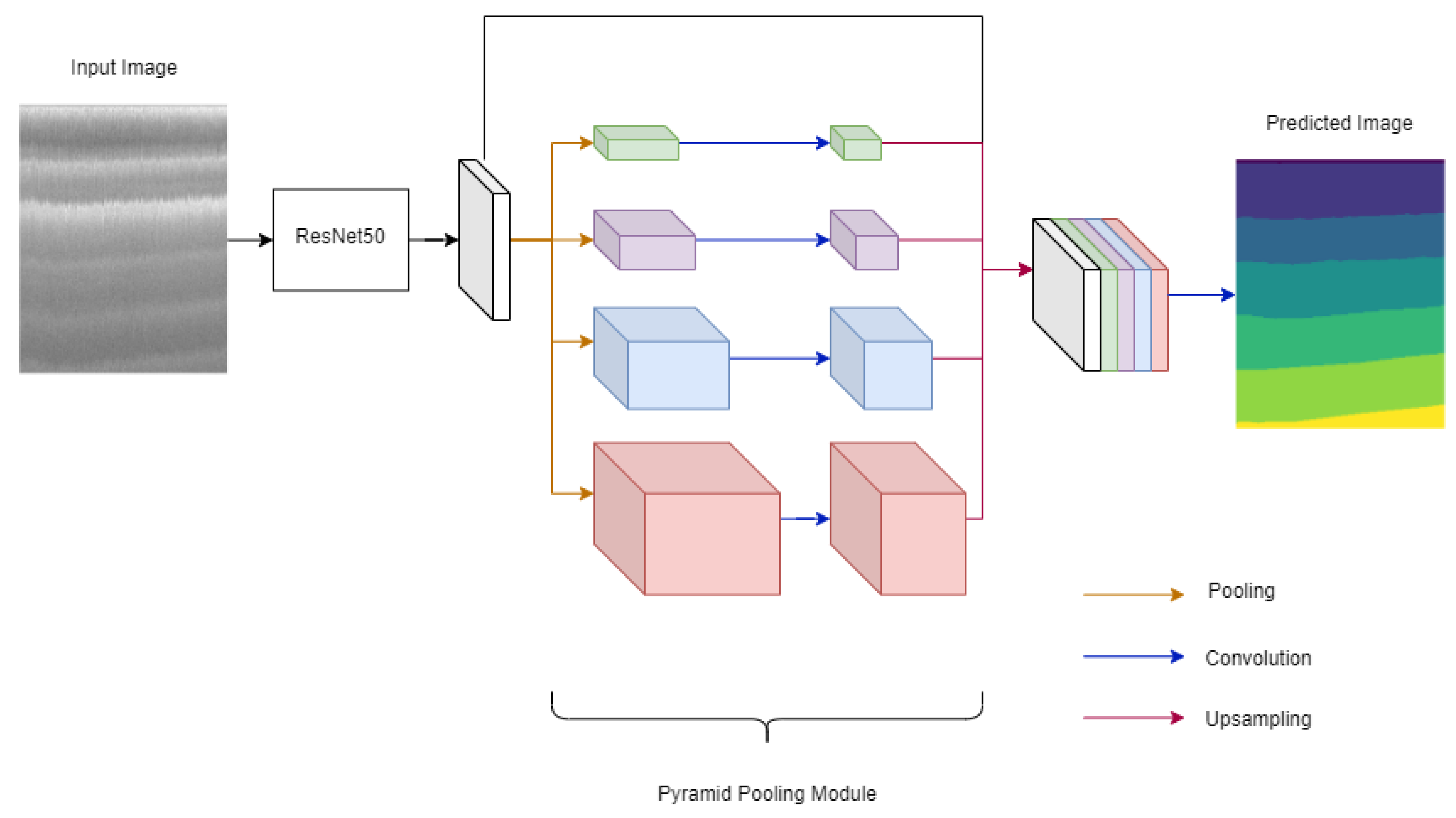
4.2.2. PSPNet
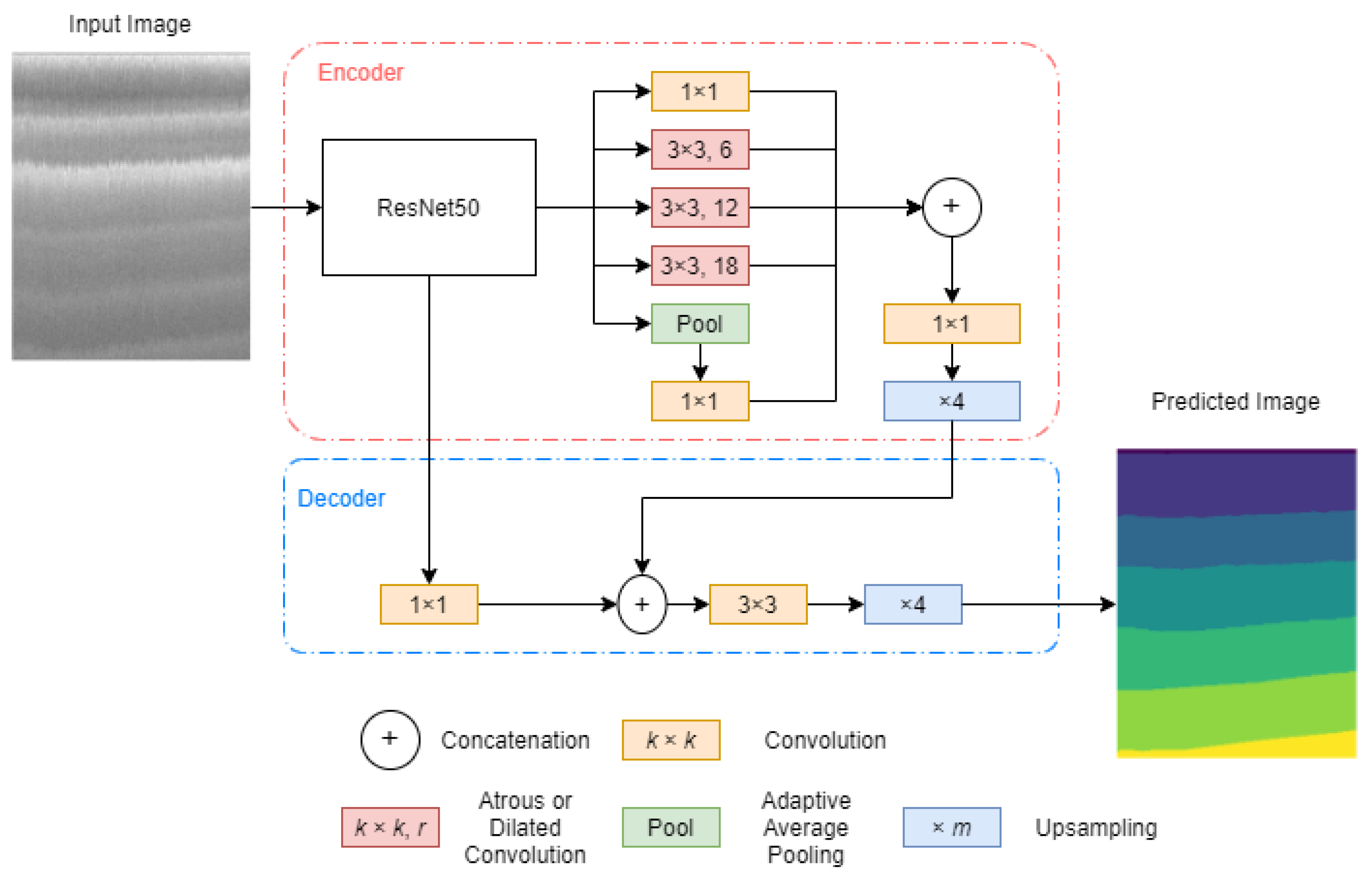
4.2.3. DeepLabv3+
4.3. Tracing of Annual Snow Accumulation Layers
5. Experimental Setup
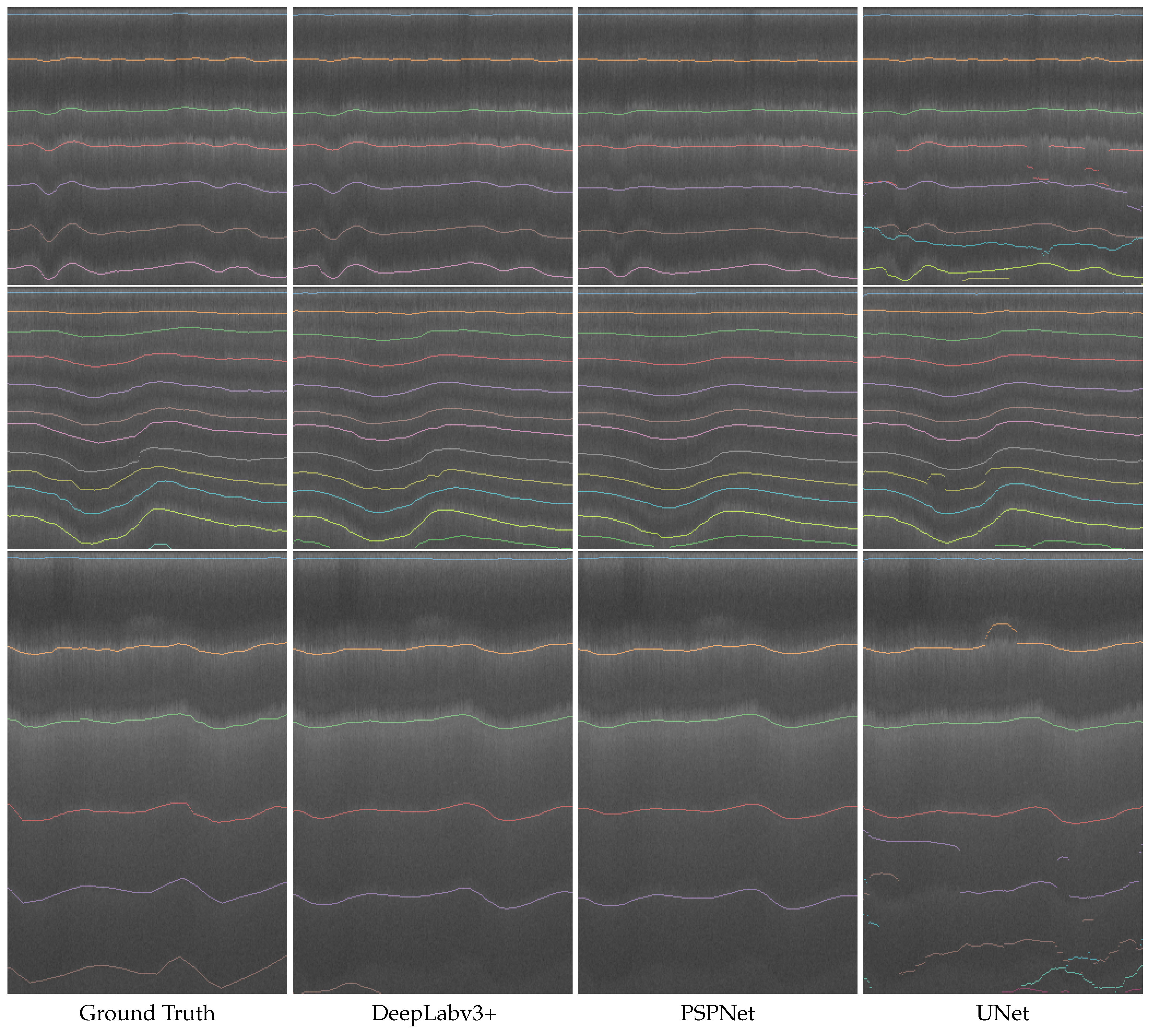
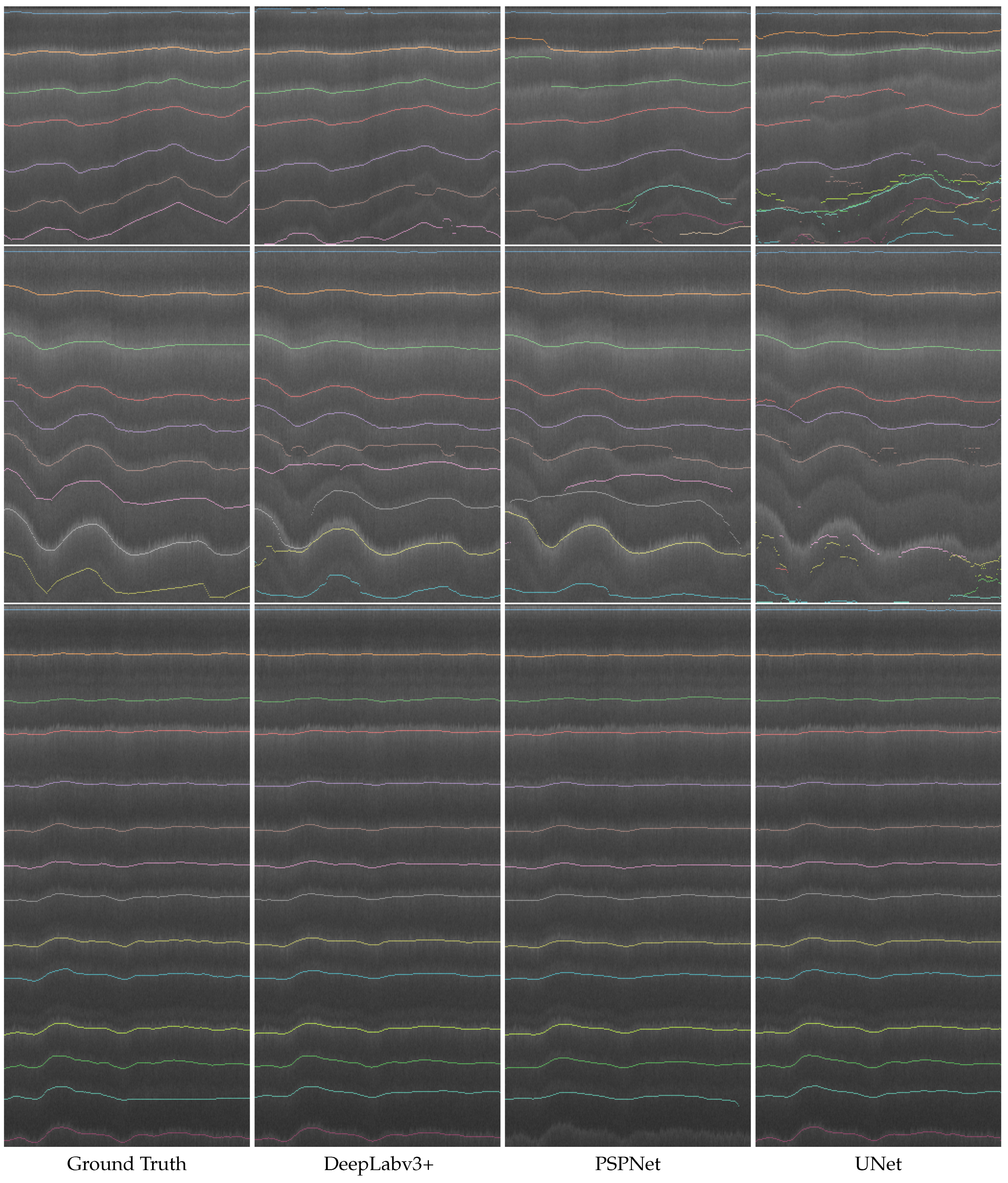
- Semantic segmentation of EG-2012:- EG’s 2012 data contains more than two thousand images having a variety of features, from those containing only the ice surface, to those having twenty to thirty internal layers. Hence, we use this data subset to find which of the three state-of-the-art FCNs will be useful for ice layer tracking. We keep 260 images for testing and the remaining 2361 for training. We train each network with two different learning rate strategies for 200 epochs each.
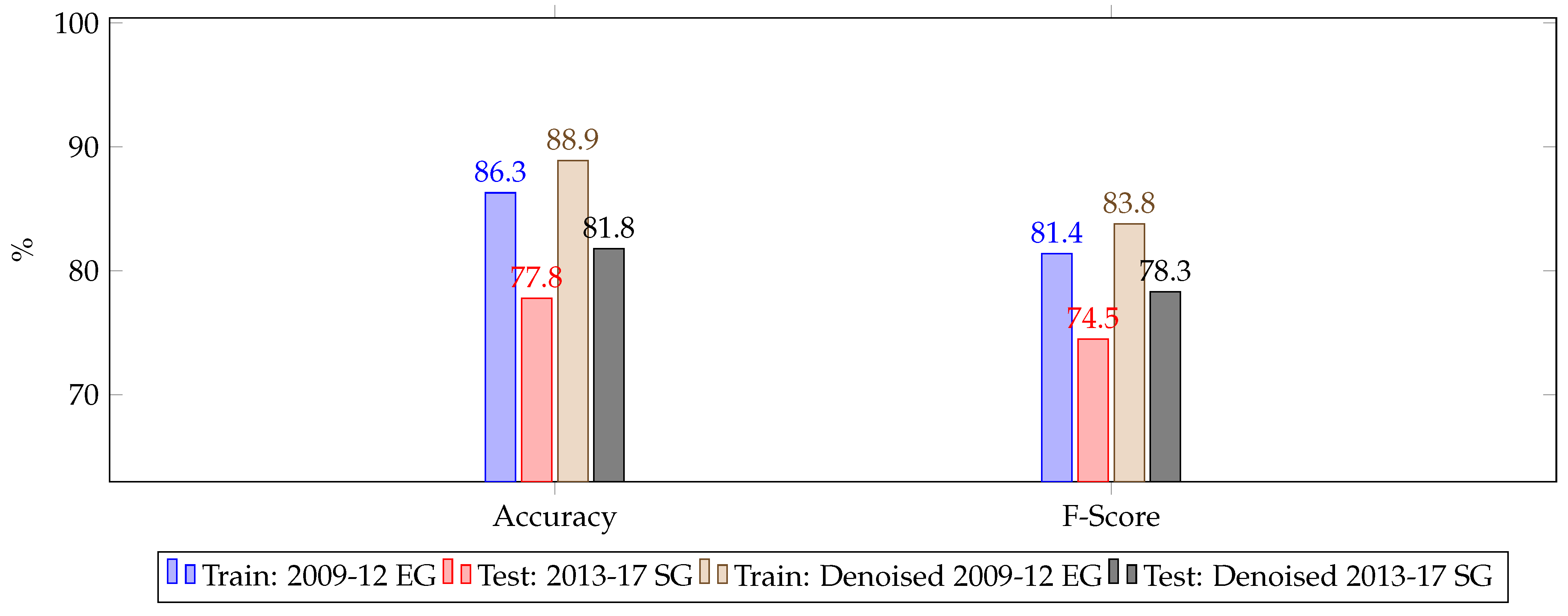
- Training on past data and predicting on future data:- For this category of experiments, we train the most generalized network obtained over EG-2012 and train it on the entire EG dataset, i.e., over the years 2009 to 2012. We then predict the ice layers on ‘future years’, 2013–2017, from the SG dataset. Training on past data before 2012, and testing on data post-2012, would give us a sense of applicability of our current method for future datasets, in general. We train on past years of EG and not of SG because the former has a larger, and varied, number of images. Further, we experiment with denoising all the images before feeding them into the FCN in order to improve layer detection. In this category, we train the network for 70 epochs.
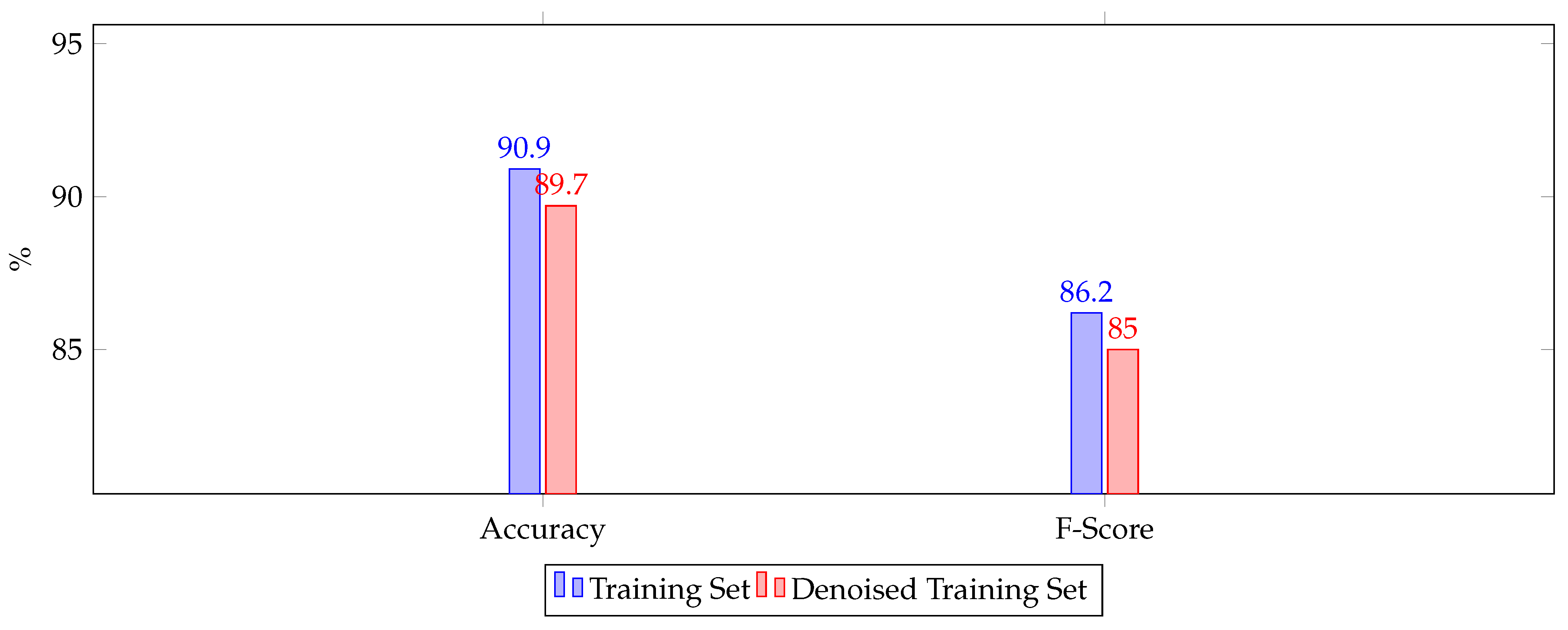
- Training and testing on combined dataset:- Here, we use the network which gave the least mean absolute error (described below) over EG-2012 and train it on the entire Snow Radar data we have, i.e., EG and SG combined. We split the dataset into 80% for training and 20% for testing. As this is a large dataset, it would help in nourishing FCN. Here, again, we experiment with training on both regular and denoised images, for 70 epochs.
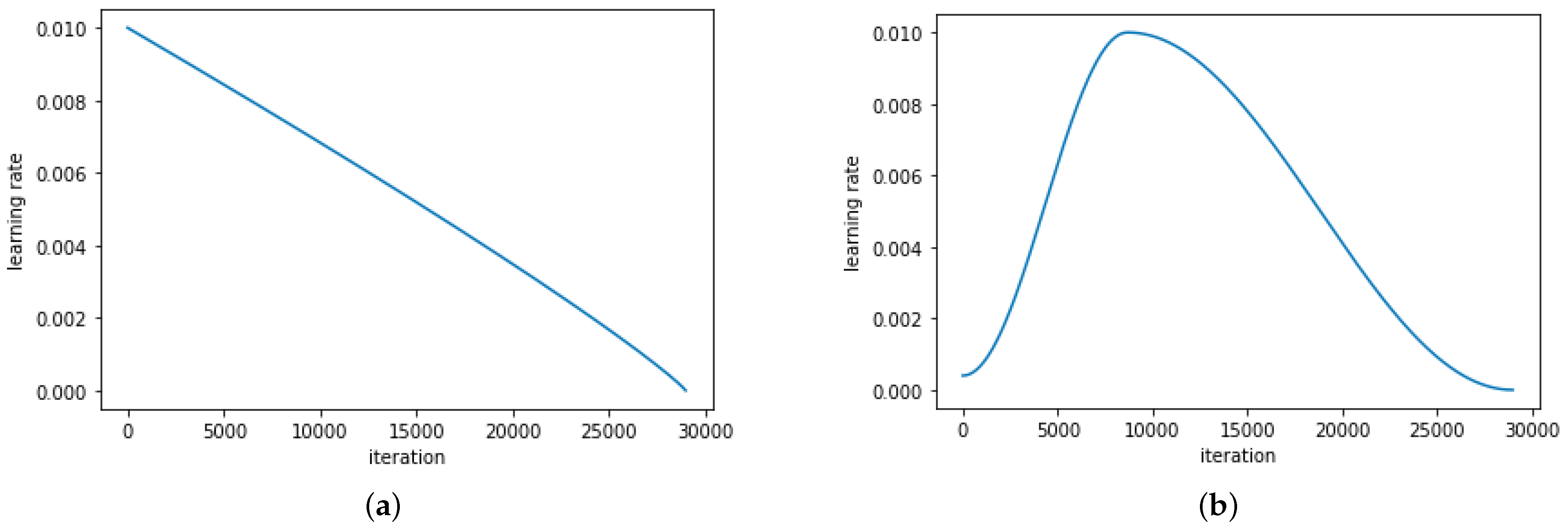
5.1. Hyperparameters
5.2. Evaluation Metrics
6. Results and Discussion
6.1. Segmentation and Thickness Estimation of EG-2012
6.2. Training on Past Data and Predicting on Future Data
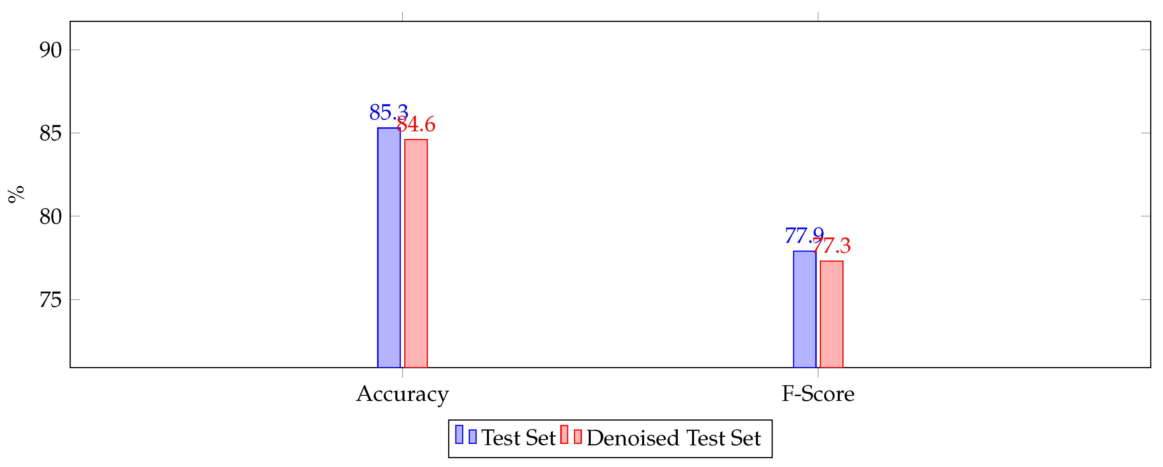
6.3. Training and Testing on Combined Dataset
7. Conclusions
Author Contributions
Funding
Data Availability Statement
Conflicts of Interest
References
- Rignot, E.; Mouginot, J.; Scheuchl, B.; van den Broeke, M.; van Wessem, M.J.; Morlighem, M. Four decades of Antarctic Ice Sheet mass balance from 1979–2017. Proc. Natl. Acad. Sci. USA 2019, 116, 1095–1103. [Google Scholar] [CrossRef] [Green Version]
- IPCC. IPCC AR5 WG1 Summary for Policymakers; IPCC: Paris, France, 2014. [Google Scholar]
- Rahnemoonfar, M.; Yari, M.; Paden, J.; Koenig, L.; Oluwanisola, I. Deep multi-scale learning for automatic tracking of internal layers of ice in radar data. J. Glaciol. 2020, 67, 39–48. [Google Scholar] [CrossRef]
- Gogineni, S.; Yan, J.B.; Gomez, D.; Rodriguez-Morales, F.; Paden, J.; Leuschen, C. Ultra-wideband radars for remote sensing of snow and ice. In Proceedings of the IEEE MTT-S International Microwave and RF Conference, New Delhi, India, 14–16 December 2013; pp. 1–4. [Google Scholar]
- Koenig, L.S.; Ivanoff, A.; Alexander, P.M.; MacGregor, J.A.; Fettweis, X.; Panzer, B.; Paden, J.D.; Forster, R.R.; Das, I.; McConnell, J.R.; et al. Annual Greenland accumulation rates (2009–2012) from airborne snow radar. Cryosphere 2016, 10, 1739–1752. [Google Scholar] [CrossRef] [Green Version]
- Arnold, E.; Leuschen, C.; Rodriguez-Morales, F.; Li, J.; Paden, J.; Hale, R.; Keshmiri, S. CReSIS airborne radars and platforms for ice and snow sounding. Ann. Glaciol. 2019, 1–10. [Google Scholar] [CrossRef] [Green Version]
- MacGregor, J.A.; Fahnestock, M.A.; Catania, G.A.; Paden, J.D.; Prasad Gogineni, S.; Young, S.K.; Rybarski, S.C.; Mabrey, A.N.; Wagman, B.M.; Morlighem, M. Radiostratigraphy and age structure of the Greenland Ice Sheet. J. Geophys. Res. Earth Surf. 2015, 120, 212–241. [Google Scholar] [CrossRef] [PubMed] [Green Version]
- Rahnemoonfar, M.; Johnson, J.; Paden, J. AI Radar Sensor: Creating Radar Depth Sounder Images Based on Generative Adversarial Network. Sensors 2019, 19, 5479. [Google Scholar] [CrossRef] [Green Version]
- Yari, M.; Rahnemoonfar, M.; Paden, J.; Oluwanisola, I.; Koenig, L.; Montgomery, L. Smart Tracking of Internal Layers of Ice in Radar Data via Multi-Scale Learning. In Proceedings of the 2019 IEEE International Conference on Big Data (Big Data), Los Angeles, CA, USA, 9–12 December 2019; pp. 5462–5468. [Google Scholar]
- Yari, M.; Rahnemoonfar, M.; Paden, J.; Koenig, L.; Oluwanisola, I. Multi-Scale and Temporal Transfer Learning for Automatic Tracking of Internal Ice Layers. In Proceedings of the IEEE International Geoscience and Remote Sensing Symposium, Waikoloa, HI, USA, 26 September–2 October 2020. [Google Scholar]
- LeCun, Y.; Bengio, Y.; Hinton, G. Deep learning. Nature 2015, 521, 436–444. [Google Scholar] [CrossRef]
- Fu, H.; Cheng, J.; Xu, Y.; Wong, D.W.K.; Liu, J.; Cao, X. Joint Optic Disc and Cup Segmentation Based on Multi-Label Deep Network and Polar Transformation. IEEE Trans. Med. Imaging 2018, 37, 1597–1605. [Google Scholar] [CrossRef] [Green Version]
- Ronneberger, O.; Fischer, P.; Brox, T. U-Net: Convolutional Networks for Biomedical Image Segmentation. In Medical Image Computing and Computer-Assisted Intervention–MICCAI 2015; Navab, N., Hornegger, J., Wells, W.M., Frangi, A.F., Eds.; Springer International Publishing: Cham, Switzerland, 2015; pp. 234–241. [Google Scholar]
- Varshney, D.; Gupta, P.K.; Persello, C.; Nikam, B.R. Deep Convolutional Networks for Cloud Detection Using Resourcesat-2 Data. In Proceedings of the IGARSS 2019-2019 IEEE International Geoscience and Remote Sensing Symposium, Yokohama, Japan, 28 July–2 August 2019; pp. 9851–9854. [Google Scholar]
- Cordts, M.; Omran, M.; Ramos, S.; Rehfeld, T.; Enzweiler, M.; Benenson, R.; Franke, U.; Roth, S.; Schiele, B. The Cityscapes Dataset for Semantic Urban Scene Understanding. In Proceedings of the IEEE Conference on Computer Vision and Pattern Recognition, Las Vegas, NV, USA, 27–30 June 2016; pp. 3213–3223. [Google Scholar]
- Carrer, L.; Bruzzone, L. Automatic Enhancement and Detection of Layering in Radar Sounder Data Based on a Local Scale Hidden Markov Model and the Viterbi Algorithm. IEEE Trans. Geosci. Remote Sens. 2017, 55, 962–977. [Google Scholar] [CrossRef]
- Ferro, A.; Bruzzone, L. Automatic Extraction and Analysis of Ice Layering in Radar Sounder Data. IEEE Trans. Geosci. Remote Sens. 2013, 51, 1622–1634. [Google Scholar] [CrossRef]
- Ilisei, A.; Bruzzone, L. A System for the Automatic Classification of Ice Sheet Subsurface Targets in Radar Sounder Data. IEEE Trans. Geosci. Remote Sens. 2015, 53, 3260–3277. [Google Scholar] [CrossRef]
- Rahnemoonfar, M.; Fox, G.C.; Yari, M.; Paden, J. Automatic Ice Surface and Bottom Boundaries Estimation in Radar Imagery Based on Level-Set Approach. IEEE Trans. Geosci. Remote Sens. 2017, 55, 5115–5122. [Google Scholar] [CrossRef]
- Rahnemoonfar, M.; Habashi, A.A.; Paden, J.; Fox, G.C. Automatic Ice thickness estimation in radar imagery based on charged particles concept. In Proceedings of the 2017 IEEE International Geoscience and Remote Sensing Symposium (IGARSS), Fort Worth, TX, USA, 23–28 July 2017; pp. 3743–3746. [Google Scholar]
- Xu, M.; Crandall, D.J.; Fox, G.C.; Paden, J.D. Automatic estimation of ice bottom surfaces from radar imagery. In Proceedings of the 2017 IEEE International Conference on Image Processing (ICIP), Beijing, China, 17–20 September 2017; pp. 340–344. [Google Scholar]
- de Paul Onana, V.; Koenig, L.S.; Ruth, J.; Studinger, M.; Harbeck, J.P. A Semiautomated Multilayer Picking Algorithm for Ice-Sheet Radar Echograms Applied to Ground-Based Near-Surface Data. IEEE Trans. Geosci. Remote Sens. 2015, 53, 51–69. [Google Scholar] [CrossRef]
- Rahnemoonfar, M.; Yari, M.; Paden, J. Radar Sensor Simulation with Generative Adversarial Network. In Proceedings of the IEEE International Geoscience and Remote Sensing Symposium, Waikoloa, HI, USA, 26 September–2 October 2020. [Google Scholar]
- Oluwanisola, I.; Paden, J.; Rahnemoonfar, M.; Crandall, D.; Yari, M. Snow Radar Layer Tracking Using Iterative Neural Network Approach. In Proceedings of the IEEE International Geoscience and Remote Sensing Symposium, Waikoloa, HI, USA, 26 September–2 October 2020. [Google Scholar]
- Chen, L.C.; Zhu, Y.; Papandreou, G.; Schroff, F.; Adam, H. Encoder-Decoder with Atrous Separable Convolution for Semantic Image Segmentation. In Computer Vision–ECCV 2018; Ferrari, V., Hebert, M., Sminchisescu, C., Weiss, Y., Eds.; Springer International Publishing: Cham, Switzerland, 2018; pp. 833–851. [Google Scholar]
- Zhao, H.; Shi, J.; Qi, X.; Wang, X.; Jia, J. Pyramid Scene Parsing Network. In Proceedings of the IEEE Conference on Computer Vision and Pattern Recognition (CVPR), Honolulu, HI, USA, 21–26 July 2017. [Google Scholar]
- CReSIS. NASA OIB Greenland 2009–2012. Available online: https://data.cresis.ku.edu/data/temp/internal_layers/NASA_OIB_test_files/image_files/greenland_picks_final_2009_2012_reformat/ (accessed on 1 June 2021).
- CReSIS. NASA OIB Greenland 2009–2017. Available online: https://data.cresis.ku.edu/data/temp/internal_layers/NASA_OIB_test_files/image_files/Corrected_SEGL_picks_lnm_2009_2017_reformat/ (accessed on 1 June 2021).
- Montgomery, L.; Koenig, L.; Lenaerts, J.T.M.; Kuipers Munneke, P. Accumulation rates (2009–2017) in Southeast Greenland derived from airborne snow radar and comparison with regional climate models. Ann. Glaciol. 2020, 61, 225–233. [Google Scholar] [CrossRef] [Green Version]
- Zhang, K.; Li, Y.; Zuo, W.; Zhang, L.; Van Gool, L.; Timofte, R. Plug-and-play image restoration with deep denoiser prior. arXiv 2020, arXiv:2008.13751. [Google Scholar]
- He, K.; Zhang, X.; Ren, S.; Sun, J. Deep Residual Learning for Image Recognition. In Proceedings of the 2016 IEEE Conference on Computer Vision and Pattern Recognition (CVPR), Las Vegas, NV, USA, 27–30 June 2016; pp. 770–778. [Google Scholar]
- Guan, S.; Khan, A.A.; Sikdar, S.; Chitnis, P.V. Fully Dense UNet for 2-D Sparse Photoacoustic Tomography Artifact Removal. IEEE J. Biomed. Health Inform. 2020, 24, 568–576. [Google Scholar] [CrossRef] [PubMed] [Green Version]
- Weng, Y.; Zhou, T.; Li, Y.; Qiu, X. NAS-Unet: Neural Architecture Search for Medical Image Segmentation. IEEE Access 2019, 7, 44247–44257. [Google Scholar] [CrossRef]
- Jiao, L.; Huo, L.; Hu, C.; Tang, P. Refined UNet: UNet-Based Refinement Network for Cloud and Shadow Precise Segmentation. Remote Sens. 2020, 12, 2001. [Google Scholar] [CrossRef]
- Cui, B.; Chen, X.; Lu, Y. Semantic Segmentation of Remote Sensing Images Using Transfer Learning and Deep Convolutional Neural Network with Dense Connection. IEEE Access 2020, 8, 116744–116755. [Google Scholar] [CrossRef]
- Baheti, B.; Innani, S.; Gajre, S.; Talbar, S. Eff-UNet: A Novel Architecture for Semantic Segmentation in Unstructured Environment. In Proceedings of the IEEE/CVF Conference on Computer Vision and Pattern Recognition (CVPR) Workshops, Seattle, WA, USA, 14–19 June 2020. [Google Scholar]
- Lee, C.Y.; Xie, S.; Gallagher, P.; Zhang, Z.; Tu, Z. Deeply-Supervised Nets. In Proceedings of Machine Learning Research, Proceedings of the Eighteenth International Conference on Artificial Intelligence and Statistics, San Diego, CA, USA, 9–12 May 2015; Lebanon, G., Vishwanathan, S.V.N., Eds.; PMLR: San Diego, CA, USA, 2015; Volume 38, pp. 562–570. [Google Scholar]
- Smith, L.N.; Topin, N. Super-convergence: Very fast training of neural networks using large learning rates. In Artificial Intelligence and Machine Learning for Multi-Domain Operations Applications; Pham, T., Ed.; International Society for Optics and Photonics (SPIE): Baltimore, MD, USA, 2019; Volume 11006, pp. 369–386. [Google Scholar]


| Dataset | Region | Timespan (Years) | Number of Images |
|---|---|---|---|
| EG | Entire Greenland | 2009 to 2012 | 21,445 |
| SG | Southeast Greenland | 2009 to 2017 | 2037 |
| EG-2012 | Entire Greenland | 2012 | 2621 |
| Network-LRS | Train | Test |
|---|---|---|
| UNet-Poly | 0.755 | 0.714 |
| UNet-OneCycle | 0.856 | 0.792 |
| PSPNet-Poly | 0.948 | 0.899 |
| PSPNet-OneCycle | 0.938 | 0.867 |
| DeepLabv3+-Poly | 0.957 | 0.887 |
| DeepLabv3+-OneCycle | 0.935 | 0.886 |
| Network-LRS | Train | Test |
|---|---|---|
| UNet-Poly | 0.387 | 0.343 |
| UNet-OneCycle | 0.549 | 0.438 |
| PSPNet-Poly | 0.737 | 0.650 |
| PSPNet-OneCycle | 0.728 | 0.589 |
| DeepLabv3+-Poly | 0.734 | 0.590 |
| DeepLabv3+-OneCycle | 0.676 | 0.595 |
| Network-LRS | Train | Test |
|---|---|---|
| UNet-Poly | 7.95 | 8.75 |
| UNet-OneCycle | 5.22 | 6.17 |
| PSPNet-Poly | 2.80 | 3.63 |
| PSPNet-OneCycle | 4.03 | 5.62 |
| DeepLabv3+-Poly | 2.36 | 3.75 |
| DeepLabv3+-OneCycle | 3.08 | 3.59 |
| Year | Vertical Pixel Size (cm) | Accuracy (%) | F-Score (%) | MAE (Pixels) |
|---|---|---|---|---|
| 2009 | 1.42 | 87.3 | 82.2 | 1.27 |
| 2010 | 1.39 | 93.5 | 88.0 | 0.75 |
| 2011 | 3.19 | 92.1 | 86.5 | 0.54 |
| 2012 | 2.07 | 90.2 | 85.1 | 1.36 |
| Year | Vertical Pixel Size (cm) | Accuracy (%) | F-Score (%) | MAE (Pixels) |
|---|---|---|---|---|
| 2009 | 1.39 | 94.8 | 88.2 | 5.97 |
| 2010 | 1.37 | 90.7 | 85.1 | 3.26 |
| 2011 | 1.54 | 87.0 | 82.1 | 2.19 |
| 2012 | 1.03 | 87.7 | 82.8 | 6.41 |
| 2013 | 2.11 | 88.5 | 83.4 | 0.98 |
| 2014 | 1.03 | 89.3 | 84.2 | 2.01 |
| 2015 | 1.05 | 90.2 | 85.3 | 7.25 |
| 2016 | 1.05 | 89.6 | 85.1 | 7.28 |
| 2017 | 0.83 | 89.8 | 85.3 | 5.79 |
Publisher’s Note: MDPI stays neutral with regard to jurisdictional claims in published maps and institutional affiliations. |
© 2021 by the authors. Licensee MDPI, Basel, Switzerland. This article is an open access article distributed under the terms and conditions of the Creative Commons Attribution (CC BY) license (https://creativecommons.org/licenses/by/4.0/).
Share and Cite
Varshney, D.; Rahnemoonfar, M.; Yari, M.; Paden, J.; Ibikunle, O.; Li, J. Deep Learning on Airborne Radar Echograms for Tracing Snow Accumulation Layers of the Greenland Ice Sheet. Remote Sens. 2021, 13, 2707. https://doi.org/10.3390/rs13142707
Varshney D, Rahnemoonfar M, Yari M, Paden J, Ibikunle O, Li J. Deep Learning on Airborne Radar Echograms for Tracing Snow Accumulation Layers of the Greenland Ice Sheet. Remote Sensing. 2021; 13(14):2707. https://doi.org/10.3390/rs13142707
Chicago/Turabian StyleVarshney, Debvrat, Maryam Rahnemoonfar, Masoud Yari, John Paden, Oluwanisola Ibikunle, and Jilu Li. 2021. "Deep Learning on Airborne Radar Echograms for Tracing Snow Accumulation Layers of the Greenland Ice Sheet" Remote Sensing 13, no. 14: 2707. https://doi.org/10.3390/rs13142707
APA StyleVarshney, D., Rahnemoonfar, M., Yari, M., Paden, J., Ibikunle, O., & Li, J. (2021). Deep Learning on Airborne Radar Echograms for Tracing Snow Accumulation Layers of the Greenland Ice Sheet. Remote Sensing, 13(14), 2707. https://doi.org/10.3390/rs13142707