Abstract
Obtaining high-quality precipitation datasets with a fine spatial resolution is of great importance for a variety of hydrological, meteorological and environmental applications. Satellite-based remote sensing can measure precipitation in large areas but suffers from inherent bias and relatively coarse resolutions. Based on the high accuracy surface modeling method (HASM), this study proposed a new downscaling method, the high accuracy surface modeling-based downscaling method (HASMD), to derive high-quality monthly precipitation estimates at a spatial resolution of 0.01° by downscaling the Integrated Multi-satellitE Retrievals for Global Precipitation Measurement (IMERG) precipitation estimates in China. A scale transformation equation was introduced in HASMD, and the initial value was set by including the explanatory variables related to precipitation. The performance of HASMD was evaluated by comparing the results yielded by HASM and the combined method of HASM, Kriging, IDW and the geographical weighted regression (GWR) method (GWR-HASM, GWR-Kriging, GWR-IDW). Analysis results indicated that HASMD performed better than the other four methods. High agreement was achieved for HASMD, with bias values ranging from 0.07 to 0.29, root mean square error (RMSE) values ranging from 9.53 mm to 47.03 mm, and R2 values ranging from 0.75 to 0.96. Compared with the original IMERG precipitation products, the downscaling accuracy with HASMD improved up to 47%, 47%, and 14% according to bias, RMSE and R2, respectively. HASMD was able to capture the spatial variation in monthly precipitation in a vast region, and it might be potentially applicable for enhancing the spatial resolution and accuracy of remotely sensed precipitation data and facilitating their application at large scales.
1. Introduction
Precipitation plays a key role in multidisciplinary scientific and application fields, such as hydrology, meteorology, and climate change. Accurate precipitation estimates with fine spatial resolution are essential to improve our understanding of most hydrometeorological and eco-environmental processes [1,2,3]. Satellite remote sensing has been proved as a significant method for obtaining spatially continuous and large-scale precipitation information. However, the low spatial resolution of satellite-based precipitation products may not be conducive to managing water resources and quantifying ecological and hydrological processes. For example, the most advanced satellite-based precipitation estimates of the Global Precipitation Mission (GPM) are available at a half-hourly scale with a relatively coarse resolution of 0.1° [4,5,6]. The performance of the Integrated Multi-satellitE Retrievals for GPM (IMERG) varies with region, exhibiting good quality in most regions of China and degraded quality in cold climates [7,8,9]. Previous studies showed that snowfall estimates of IMERG have poor accuracy, partly resulting in their degraded performance in winter. The poor performance in cold climates may be due to the few gauge observations and the snowfall retrieval algorithm [7]. Satellite-based precipitation estimates still need further improvement regarding the uncertainties and the coarse spatial resolutions. Obtaining reliable precipitation information at high spatial resolution remains a challenge, particularly in large regions with large precipitation variability.
Downscaling can be an important and effective way to retrieve fine-scale precipitation information from other coarse-resolution precipitation datasets [10,11,12,13]. Dynamic and statistical downscaling are the two main approaches to yield precipitation information with sufficient spatial details. Dynamic downscaling requires running complex climate models by integrating ocean–atmosphere–land coupled processes, which are computationally intensive and inefficient in many physical processes [14,15]. As an alternative, statistical downscaling is highly efficient and widely used to develop a relationship between precipitation and explanatory variables [10,11,16,17]. Although many statistical downscaling methods have been developed in recent years, the most popular approach is the transfer function, which is a regression-based framework. The results of these statistical downscaling approaches are typically affected by the selected explanatory variables and the established statistical relationships [13,18]. More recently, the use of machine learning methods has been increased in precipitation downscaling because of their superior performance and robust implementations [19,20,21,22]. However, as indicated by other studies [23,24], machine learning methods are usually employed to establish global numeric relationships between variables without considering the geographical laws, which means that the environmental variables are spatially correlated with themselves and the relationship between environmental parameters varies in space. An appropriate downscaling approach is still required for obtaining improved precipitation estimates.
Previous studies have indicated that a partial differential equation (PDE)-based approach could be an effective way to reduce the uncertainty in environmental variable simulations [25,26]. In the early 1970s, researchers proposed the concept of representing surfaces as solutions for PDEs and developed related algorithms [27,28]. Recently, Yue presented a high accuracy surface modeling method (HASM) in terms of the fundamental theorem of surfaces in differential geometry [26]. This theorem shows that a surface can be determined by the first and second fundamental coefficients that satisfy the Gaussian equation set [26]. By integrating the spatial autocorrelation of the variable of interest, the characteristics of spatial variation of the variable using the Gaussian equation set and a constrained equation, HASM has been successfully used in spatial interpolating of environmental variables, such as elevation, climate variables, and soil properties. Researchers have found that, in most cases, HASM performed better than other classic interpolation methods, such as the Inverse Distance Weighting method (IDW), ordinary Kriging, and spline method [11,26,29,30,31,32,33,34,35,36]. HASM, with its superior performance, is expected to have broad application prospects in estimating climatic quantities.
In recent years, Zhao performed statistical downscaling by combining the geographical weighted regression method and residual correction using a HASM-based interpolator [35]. The result of this method, abbreviated as GWR-HASM, is mainly determined by the regression method, and the residual correction by using HASM plays a supplementary role in the improvement of the final downscaling result [34,35,36]. As an interpolation method, HASM does not take into account the scale effects and auxiliary variables when it is used to downscale the remotely sensed precipitation datasets. To take advantage of the high accuracy of HASM and to promote its application, a new downscaling method, the high accuracy surface modeling-based downscaling method (HASMD), was proposed in this study. Considering the influence of the scale effect in downscaling, a scale transformation equation was introduced in HASMD. In addition, the auxiliary information of the variables was taken into account in HASMD to yield better downscaling results.
The goal of this study was to provide a new downscaling method, HASMD, to obtain high accuracy and high resolution precipitation estimates. The IMERG precipitation dataset was downscaled through an introduction of an equation for scale transformation and a modification of the initial value by considering the explanatory variables of precipitation in HASMD. The auxiliary variables include the difference vegetation index (NDVI), elevation, slope, longitude and latitude. A high-density meteorological station network with more than 2000 stations across China was used to construct the constrained equation of HASMD. The performance of HASMD was validated by using the cross validation method. The proposed downscaling method, HASMD, considers the geographical laws and is expected to provide an alternative way for enhancing the spatial resolution and accuracy of satellite-based precipitation products and facilitate their applications over a large area.
2. Study Area and Data
2.1. Study Area
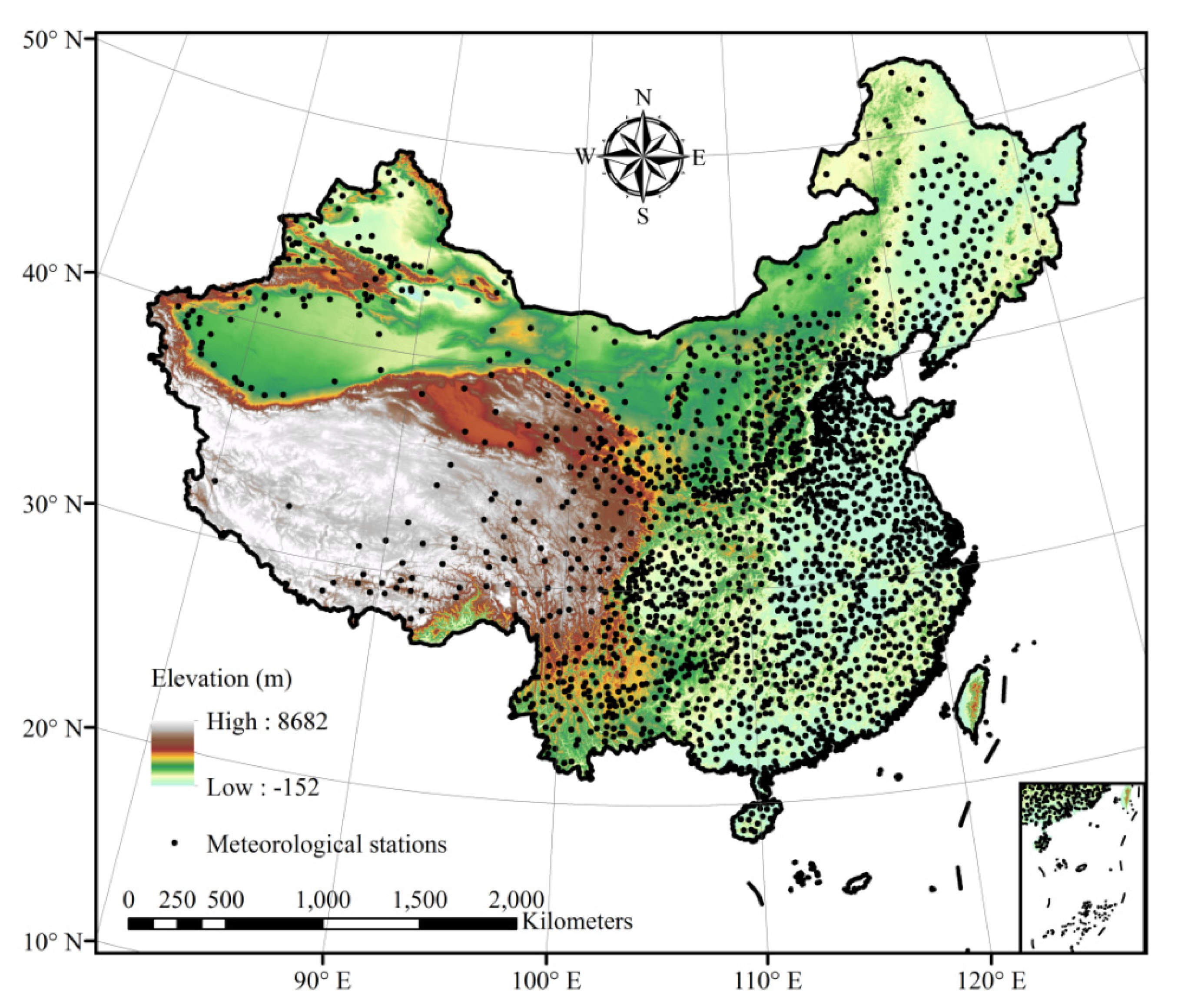
The study area, China, is located in the western Pacific and eastern Asia. Nearly two-thirds of its land area is covered by mountains, plateaus and hills, with altitudes ranging from −152 m in the northwest to higher than 8000 m in the Tibetan Plateau (Figure 1). Due to the vast area and the high variations in topography in China, the climate is complex and exhibits strong spatial heterogeneity (Figure 2). Precipitation varies greatly in space, with annual precipitation amounts of more than 2000 mm in the southeast and less than 50 mm in the northwest, which is typically influenced by the East Asian monsoon and topography (Figure 2a). More than 50% of the precipitation occurs during summer (from June to August), and precipitation in winter (January, February, and December) accounts for less than 10% of the total annual precipitation amount (Figure 2b).
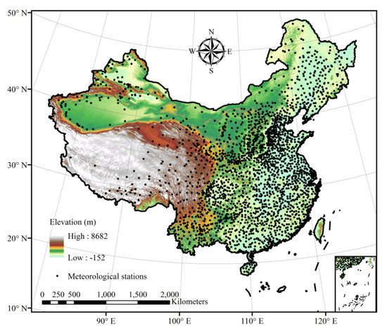
Figure 1.
Meteorological stations and elevation in China (most stations located in the south part of China).
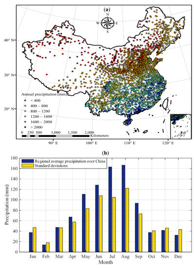
Figure 2.
Spatial–temporal variations in precipitation in China: (a) spatial distribution of annual precipitation; (b) monthly precipitation (annual precipitation amounts of more than 2000 mm were observed in the southeast and less than 50 mm in the northwest; more than 50% of the precipitation occurs during summer).
2.2. Station Observations and Satellite Precipitation Products
The in situ ground-based precipitation observations in the year 2018 were derived from the China Meteorological Data Service Center, which passed through a strict quality control by applying the software RHtests (https://github.com/ECCC-CDAS/RHtests; 1 July 2019). Combined with the station metadata, the RHtest software was used to detect and adjust artificial shifts of the monthly total precipitation of China. The center measures daily precipitation at 2419 meteorological sites, containing 839 national stations available for public use and 1580 other provincial and municipal sites. The stations are distributed unevenly across China, with most of them located in the central and eastern parts and few stations located in high mountainous areas in western China (Figure 1). These observations have undergone strict quality control and have been used to calculate monthly total precipitation in this study.
The IMERG algorithm was released in early 2015 and the IMERG version (V3) precipitation products have been provided by NASA since March 2014. The IMERG algorithm is designed to intercalibrate, merge, and interpolate all satellite microwave precipitation estimates at relatively fine temporal and spatial scales for the Tropical Rainfall Measuring Mission (TRMM) and GPM eras over the entire globe [37,38]. The recently updated retrospective IMERG in the TRMM era was released as version 06, initially started in June 2000, and continued until now. The accuracy of IMERG precipitation products has been improved from 2001 to 2018 due to the increasing number of passive microwave samples. These products have quasi-global coverage from 65°S to 65°N, with a spatial resolution of 0.1° × 0.1° and a temporal resolution of 1 day. The IMERG V06 precipitation datasets can be obtained from https://disc.gsfc.nasa.gov/datasets/GPM_3IMERGDF_06/summary?keywords=GPM; 1 October 2020).
3. Methods
3.1. The HASM-Based Downscaling Method
According to the theory of the differential geometry of surfaces, a surface can be determined by the first and second fundamental coefficients [39,40,41]. The first fundamental coefficients of a surface, , can be expressed as:
where , and denote the information about the geodesic curvature, the length of the curves, and other intrinsic geometric properties. and represent the first partial derivatives of the graph with respect to and directions, respectively. The second fundamental coefficients , and characterize the local structures of the surface and can be given as [42,43]:
where and denote the second partial derivatives of the graph with respect to and directions, respectively; is the mixed partial derivatives of the graph .
Based on the theorem of surfaces, the first and second fundamental coefficients should satisfy the Gaussian equations, so that a surface can be determined [39]. The assumption of HASM is that the spatial distribution of the predictor is deemed as a surface that can be obtained by solving the Gaussian equations. Therefore, the main equations of HASM are the following Gaussian equations:
If is the value of at the th sampled point in the computational domain, the interpolated value should be equal or approximate to the sampling value at this lattice. In order to make the interpolated value at the sampled point approximate to the real observation, a constrained equation is added to Gaussian equations (Equation (2)), and by applying Taylor expansions, the mathematical formula of HASM is lastly given by [26]:
where is a vector and each element denotes the interpolated value of the grid point; the constrained equation means that the predictor estimation is equal to the observation at each station location. Suppose there are stations in the computing region, the matrix can be given as:
where and represent the number of computing grids in and directions, respectively. That is, based on the matrix-vector multiplication, if the meteorological station, with a precipitation value of , located in the row and column in the computing grid, then , . The row number of the matrix is equal to the station number .
By applying the method of Lagrange multiplier, the HASM equations (Equation (2)) can be written as:
where is a symmetric and positive definite matrix, and . The Lagrange parameter determines the weight of the sampling points to the final results. A small value of is given in areas of complex terrain with large precipitation variations. The conjugate gradient (CG) method is an iterative method that can be used to solve matrix equations when the coefficient matrix is symmetric and positive definite [27,44,45]. However, the CG method converges fast only on matrices that are either well-conditioned or have just a few distinct eigenvalues [44,46]. The matrix in HASM is ill-conditioned, which means that the minimum eigenvalue of is approximate to zero. To improve the rate of the convergence of the CG method, a preconditioning scheme that modifies the condition of can be applied [47]. A diagonal preconditioned conjugated gradient (DPCG) method was used in this study in the inner iteration to solve Equation (3), with the stopping rule of and the stopping tolerance being equal to rather than in this study. It will be of future interest to evaluate this effect for further optimization. The calculation time of DPCG has been demonstrated to have a linear relationship with the number of the computing grids [26]. In addition, the outer iteration is used to update the right-hand vector , with the stopping criterion of the root mean square error (RMSE) reaching the minimum value for the test dataset, that is , where is the observation value at the ith point , is the solution of Equation (3) obtained from the inner iteration, is the number of test points and is the outer iteration number. By setting the initial value using a simple interpolator and constructing the constrained equation using meteorological station observations, the surface modeling of climate variables can be implemented by HASM [26,32,35].
Based on HASM, a downscaling method was developed in this study by introducing an equation of scale transformation and setting the initial value using the geographical weighted regression method (GWR) and related auxiliary variables.
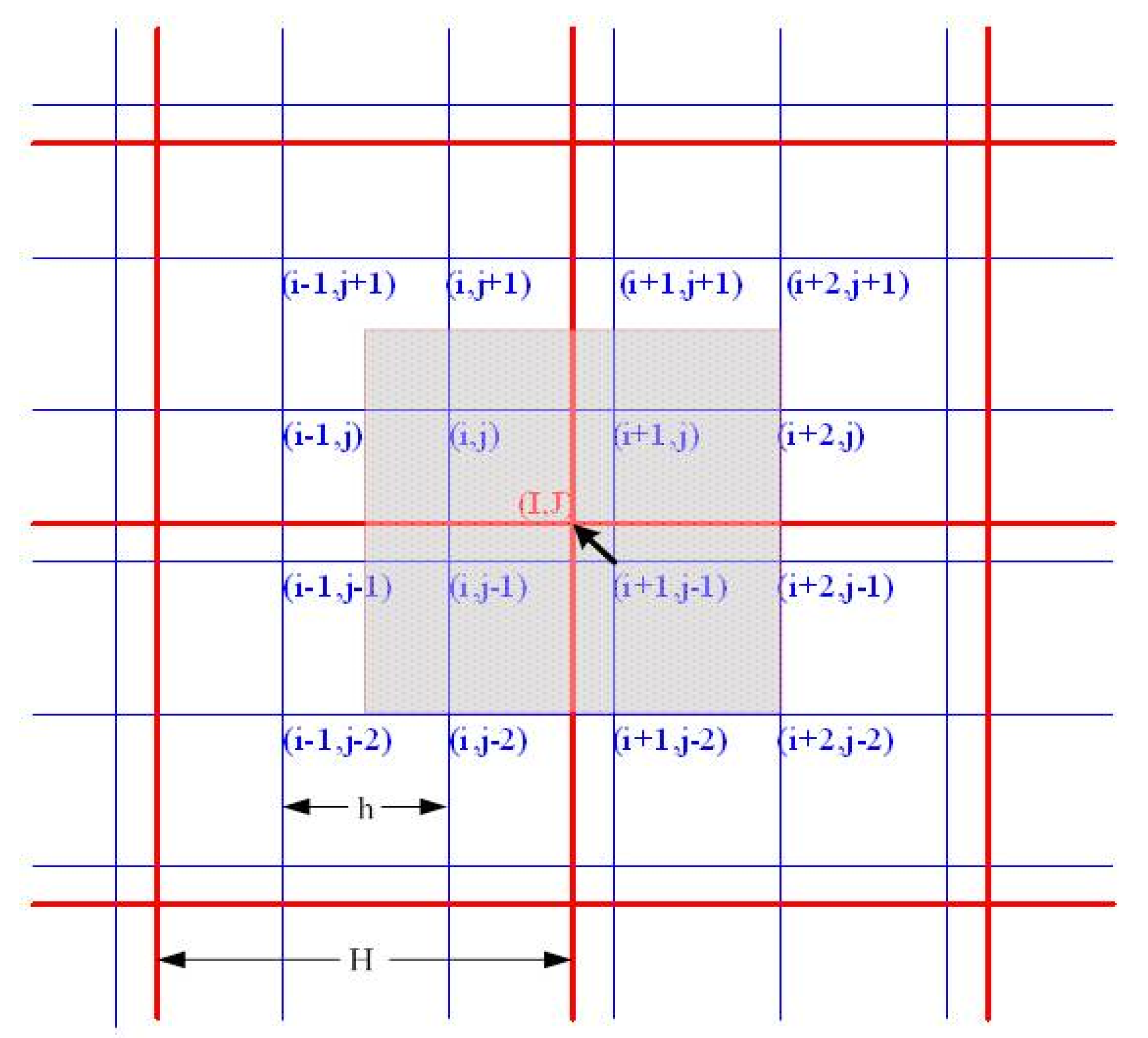
Let denote the coarse resolution and be the downscaled fine resolution (Figure 3). The equation of the scale transformation is as follows:
where denotes a transformation function and refers to the fact that the value of the coarse grid cell is the average of the values in fine grid cells, which are located in the coarse cell, that is:
where ; is the number of fine grid cells located within the same coarse grid; is the precipitation value in the coarse cell and is the downscaled precipitation value in the fine grid cell. This can be calculated by the following pseudo-codes:

Figure 3.
Stencil for scale transformation between coarse and fine grids.
| set ; ; ; |
| if the fine simulated grid cell (i,j) is located in the coarse grid (I,J), then |
| ; |
| ; |
| end |
A disadvantage of HASM is that it does not consider geographical and topographical information and only considers station observations. Although HASM takes into account the spatial autocorrelation of the variable of interest by using finite difference schemes, it ignores the correlation between the variable of interest and the related explanatory variables. Explanatory variables that correlate with the predictor, passing through the Spearman’s rank correlation test with a significance level of 1%, can be applied to improve the accuracy of HASMD. This process can be implemented by setting the initial fields using a regression method, which establishes the relationship between the explanatory variables and precipitation. In this study, we employed the local form of the regression method, GWR, to obtain the initial value of HASMD due to the large spatial variations of precipitation within mainland China.
The above can be implemented by the following problem:
where the constrained equation means that the predictor estimation is equal to the observation at each station location in the fine computing grid. Like in HASM, if the meteorological station, with a precipitation value of , located in the row and column in the fine computing grid, and . is the relationship established using the GWR method and denotes how the precipitation varies with , which represent the suitable explanatory variables. The constrained least squares problem (Equation (6)) can be changed into the following linear equation by using the method of Lagrange multipliers:
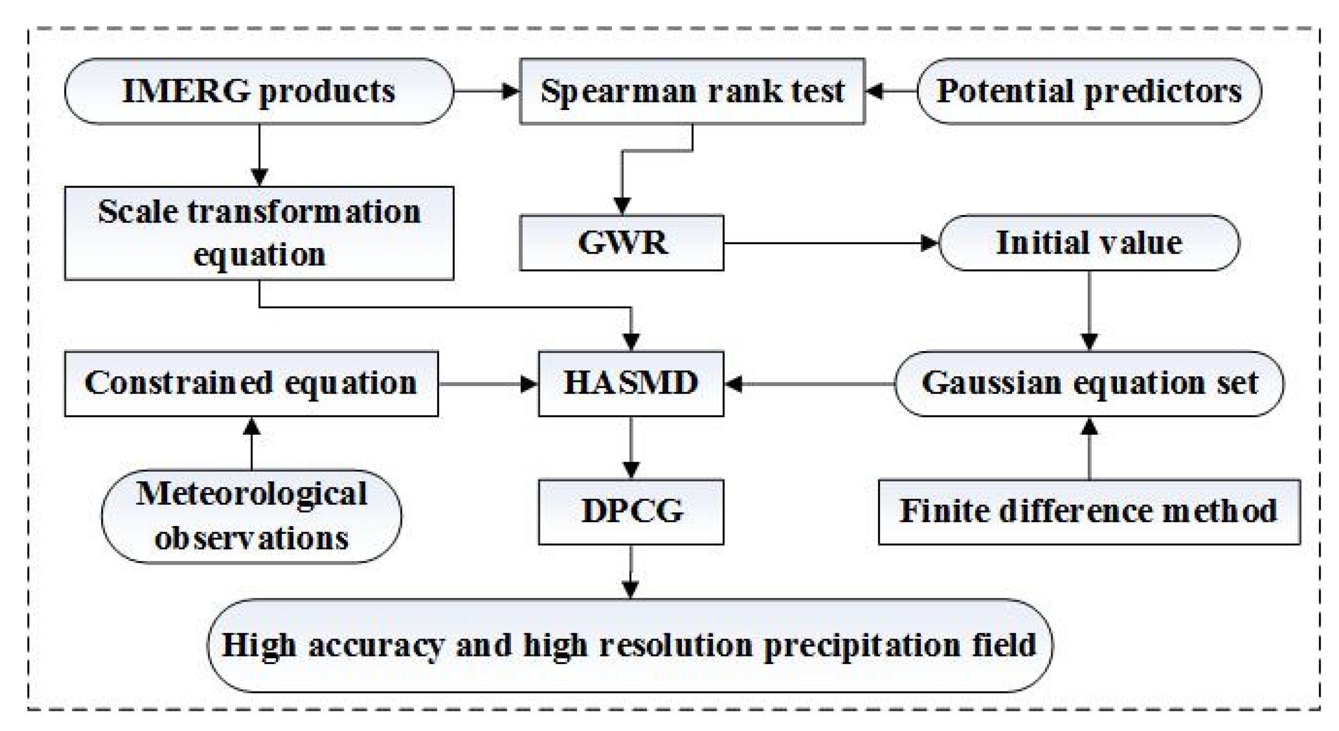
where and . is the initial value of Equation (7) with a spatial resolution of in this study; is a vector where each element denotes the precipitation value of the corresponding grid point. The solution of Equation (7) is the final precipitation estimate, which can be obtained by using the DPCG method [26]. In addition, Equation (7) means that the precipitation is firstly modified by using the GWR method with respect to explanatory variables. Then, this result was further improved by multiplying the matrix at each iteration, which, according to its calculation process, integrates the spatial autocorrelation, the variation, and the direction and slope of the variation in precipitation with respect to and directions. The downscaling scheme is presented in Figure 4.
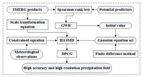
Figure 4.
Illustration of the downscaling scheme of HASMD.
Based on the modified version of HASM, abbreviated as HASMD, we downscaled the monthly IMERG precipitation products. Suitable environmental variables are important in building the downscaling model. Elevation and slope have been shown to have a direct relationship with precipitation, mainly due to orographic effects [22,48]. NDVI is widely used in satellite precipitation dataset downscaling [49,50,51,52]. Studies have indicated that there were time-lag effects between NDVI and precipitation, and these time lags varied with regions and time scales [53]. HASMD was implemented by using a suite of auxiliary variables, including NDVI, elevation, slope, longitude and latitude.
3.2. Calibration and Validation
To assess the performance of the downscaling methods, the ten-fold cross validation scheme was used in this study according to the spatial locations and temporal period, which has been widely applied in the precipitation estimation studies [54,55]. The meteorological observations were divided into two datasets by using the tool “Subset Features” in ArcGIS software: 90% of the data were used for downscaling calculations, and 10% of the data were used to validate the results. This process was repeated 10 times to ensure the representativeness of the training samples and validation samples as far as possible. The performance of HASMD was evaluated by three indicators, including bias, root mean square error (RMSE) and the coefficients of determination ().
where is the observation value at the ith point ; is the estimation; ,; and is the number of test points.
We evaluated the performance of HASMD, HASM, the method proposed in Zhao [34] (GWR-HASM), GWR-Kriging, GWR-IDW, and the original IMERG precipitation estimates according to the values of the three comparison indices. GWR-HASM, GWR-Kriging, and GWR-IDW are combined methods for downscaling precipitation that use GWR to establish the relationship between precipitation and the explanatory variables, and then use HASM, Kriging and IDW to interpolate the residuals between the results of GWR and the ground observations, respectively. The main differences between HASM and HASMD lie in the initial value and the matrix in Equation (7) due to the scale transformation equation (Equation (4)), , which integrates the spatial correlation of the precipitation and finally has an impact on the estimated value of precipitation based on Equation (7).
4. Results
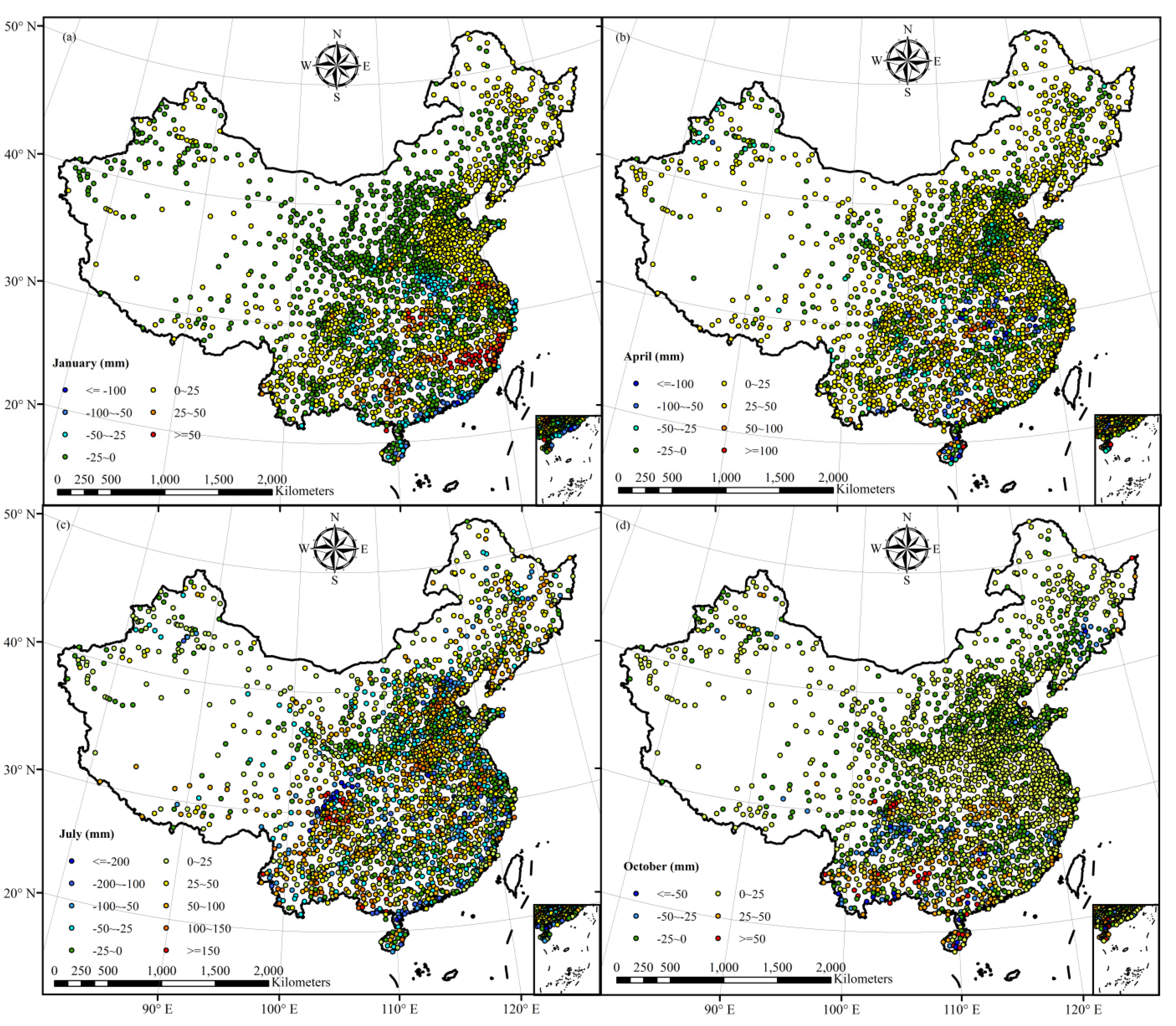
The characteristics of IMERG precipitation products were investigated at a monthly scale using the latest available data in January, April, July and October 2018, for the four examples, which represent the winter, spring, summer and autumn, respectively (Figure 5). The errors of the IMERG precipitation vary with months across mainland China. In January, the proportion of meteorological stations where the amount of IMERG product was lower than the observation values was 51%, mainly occurring in western and northern China, as denoted in Figure 5a. The maximum values of underestimation and overestimation were both observed in the southeast coastal area, with values of more than 130 mm and 109 mm, respectively. The precipitation in July was overestimated for 65% of the meteorological stations in the IMERG products, with a maximum value of 262 mm. The maximum value of underestimation in July was 352 mm, which occurred in the Sichuan Basin. Precipitation in April and October was overestimated at 67.9% and 67.6% of the total stations, with maximum bias values of 165 mm and 138 mm, respectively (Figure 5b,d). The results indicated that, compared with other months, IMERG products exhibited more underestimations in the winter months, which may be due to the poor performance of the snowfall retrieval algorithm.
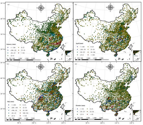
Figure 5.
The locations of the meteorological stations whose values were under- and over-estimated compared with IMERG products: (a) January; (b) April; (c) July; (d) October (the biases are represented by different colors).
Table 1 lists the precipitation errors obtained by the validation datasets for different downscaling methods in the four months. Compared with the original IMERG product, the accuracy of HASM was not clearly improved. In July and October, the RMSE values for HASM were slightly larger than those obtained using the IMERG products. The performance of HASM was better in January than in other months. For the four months, the GWR-HASM had a mean RMSE value of 26 mm, an 18% improvement compared with IMERG precipitation products. The accuracy of HASMD in January, April, July, and October was improved by 47%, 17%, 17%, and 25%, respectively, according to the RMSE values. In addition, compared with GWR-IDW, GWR-Kriging, and GWR-HASM, the mean RMSE values of HASMD were decreased by 9%, 17%, and 11%, respectively. Errors in HASMD were the smallest for the four months, indicating that HASMD yielded an obvious improvement when compared to the original IMERG precipitation estimates.

Table 1.
Errors for the downscaling results by using different methods.
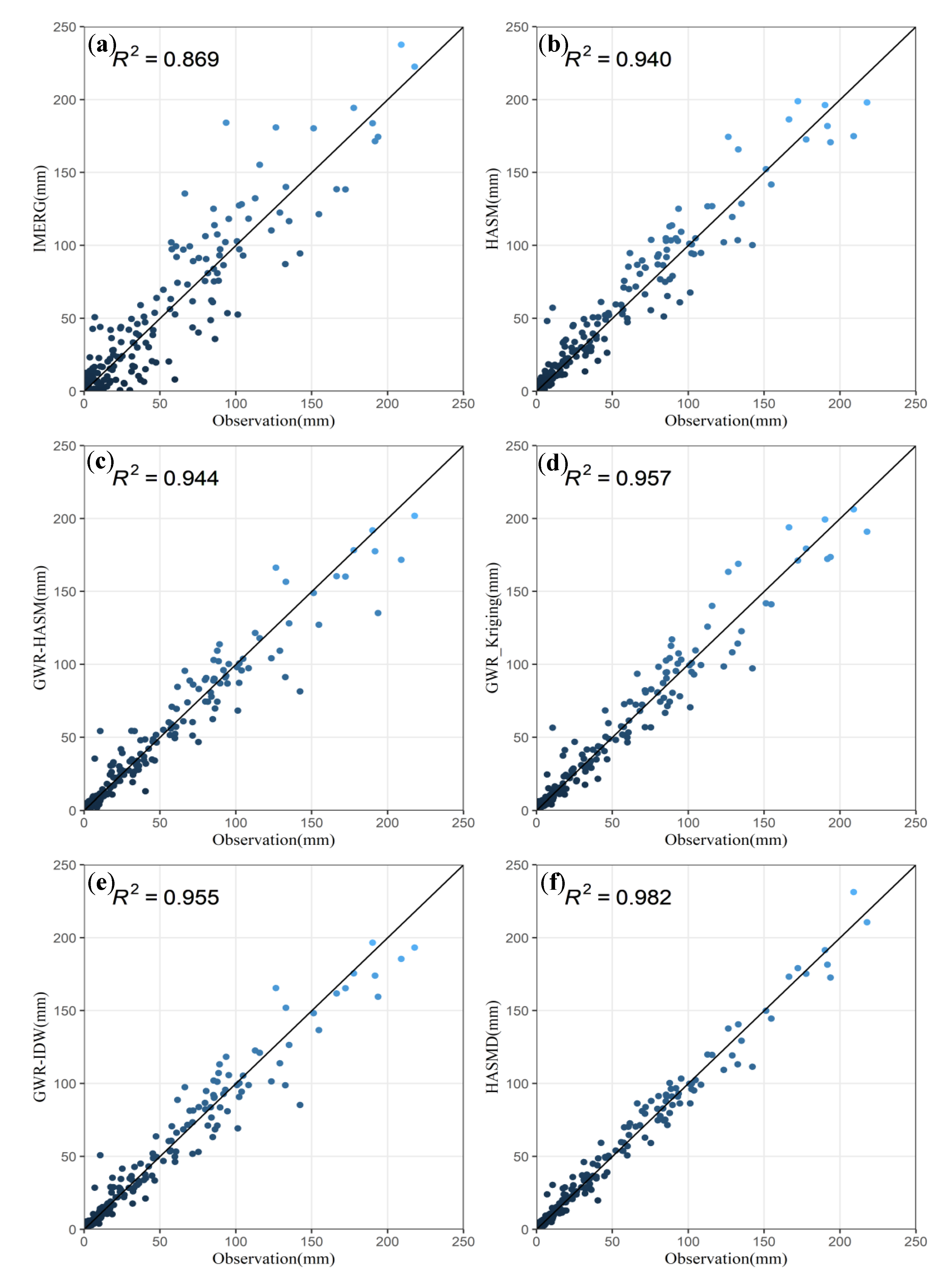
The downscaled results at 0.01° resolution using different methods in January 2018 are presented in Figure 6. The size of the point with different colors represents the absolute difference between the results of each method and the ground observations. The original IMERG product (Figure 6a) and the downscaling results showed a decreasing trend from southeast to northwest. The results of GWR-based methods (Figure 6c–e) exhibited a similar spatial pattern compared with the original IMERG product. However, large differences were observed in some local regions, especially for the HASM result (Figure 6b). Some detailed differences were also found for HASMD, such as in the northern and western parts of China, where underestimation was observed compared to the values obtained from the stations. This indicated that the HASM and HASMD methods may perform better than GWR-based methods. Validation with a random sample of 10% of the meteorological stations showed that HASMD performed better than other methods. Figure 7 displays the relationship between the 10% of the ground observations and the downscaled precipitation datasets at the corresponding stations that were extracted by using ArcGIS software in January 2018. Although the bias was modified by HASM and GWR-based methods, large underestimations and overestimations still existed compared with the original IMERG precipitation products. It is clear that HASMD performed better than the other downscaling methods, with R2 of 0.98 (p < 0.05).
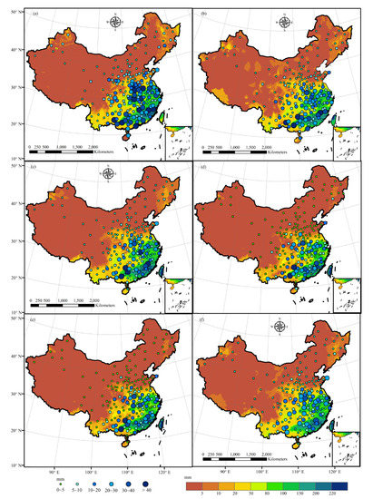
Figure 6.
Downscaling results of precipitation in January: (a) IMERG product; (b) the HASM results; (c) the GWR-HASM results; (d) the GWR-Kriging results; (e) the GWR-IDW results; (f) the HASMD results (the size of the point with different colors represents the absolute difference between the results of each method and the ground observations).
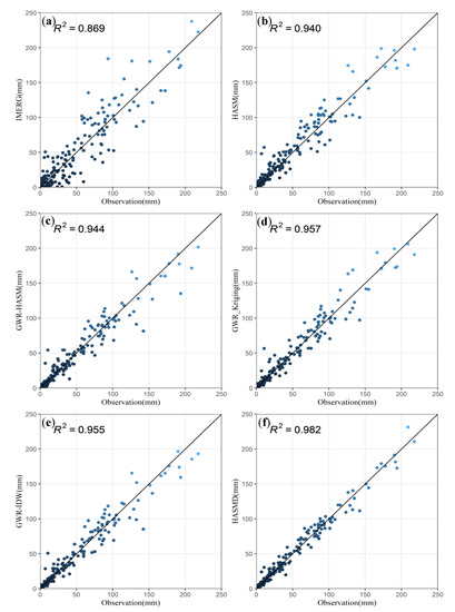
Figure 7.
Heatscatter plots of the validation between ground observations and the downscaling results in January: (a) the original IMERG product; (b) the HASM results; (c) the GWR-HASM results; (d) the GWR-Kriging results; (e) the GWR-IDW results; (f) the HASMD results.
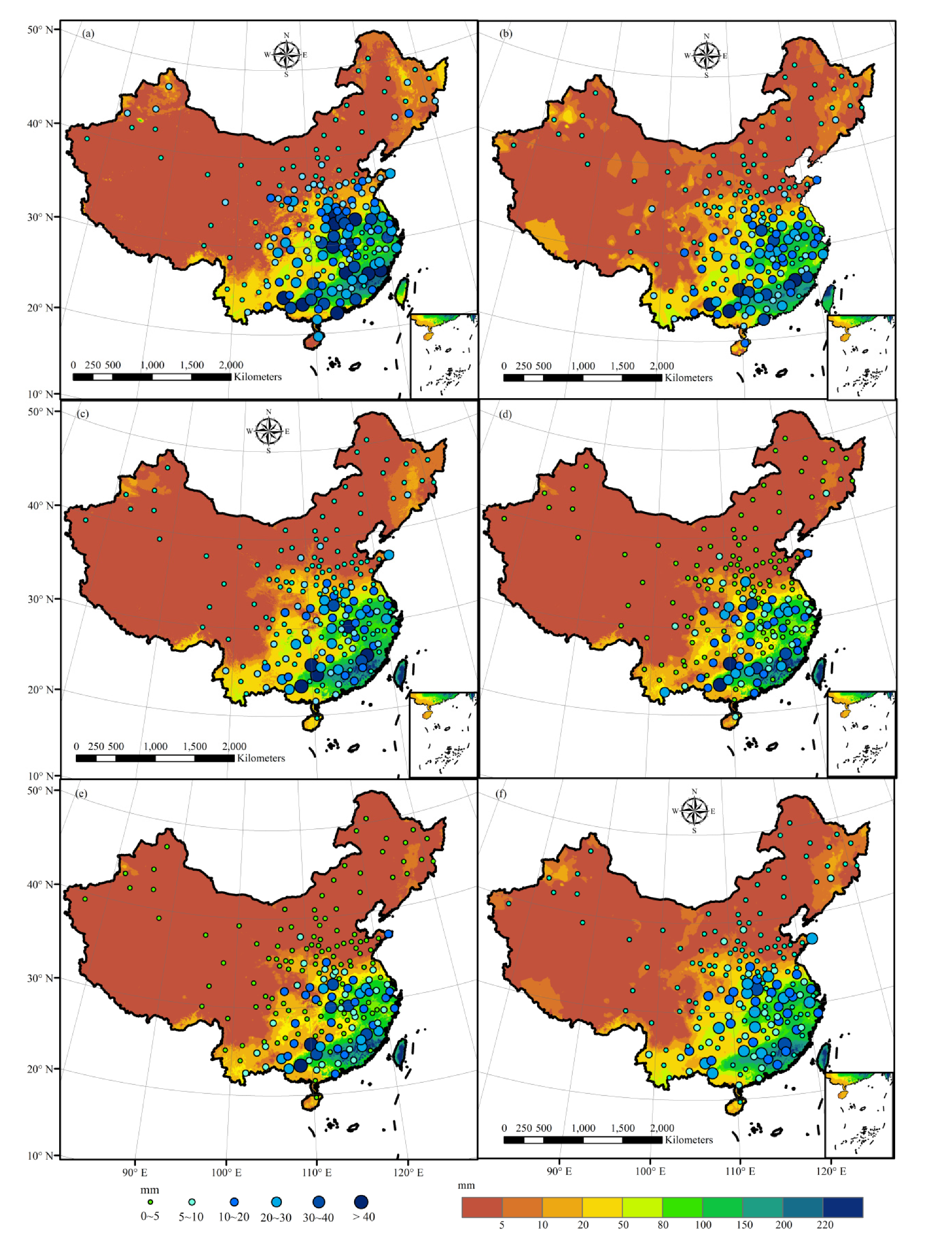
Figure 8 shows the downscaling results of the IMERG precipitation product in July. Large precipitation amounts were observed in the Sichuan Basin, south coastal region, Beijing, and parts of Heilongjiang Province. The original IMERG product and the downscaling results from HASM, GWR-based methods and HASMD displayed similar spatial patterns across China but showed different local details. The results from GWR-based methods show similar patterns and seem to agree well with the original IMERG product (Figure 8c–e). The HASM and HASMD results showed larger spatial variations than the original IMERG precipitation estimates (Figure 8b,f), and strong spatial heterogeneity was observed for HASM. Combined with the meteorological observations, it can be concluded that there might be some outliers produced by HASM. The absolute bias between the results of each method and the in-suit measurements, indicated by points with different sizes and colors, showed that HASMD performed the best. The large bias observed in the south of China was mainly due to the large precipitation amount in this area. Ten percent of the total meteorological observations were used to evaluate the downscaling results of different methods (Figure 9). The differences between the station values and the original IMERG products in July 2018 are clearly shown in Figure 9a at a significance level of 0.05. The bias of the downscaled results compared to the ground observations was still large based on the HASM and GWR-based methods. Compared to other methods, the result from HASMD agrees relatively well with the meteorological observations, followed by GWR-IDW, with R2 of 0.84 and 0.72, respectively.
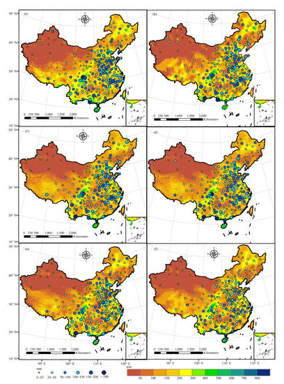
Figure 8.
Downscaling results of precipitation in July: (a) IMERG product; (b) the HASM results; (c) the GWR-HASM results; (d) the GWR-Kriging results; (e) the GWR-IDW results; (f) the HASMD results (the size of the point with different colors represents the absolute difference between the results of each method and the ground observations).
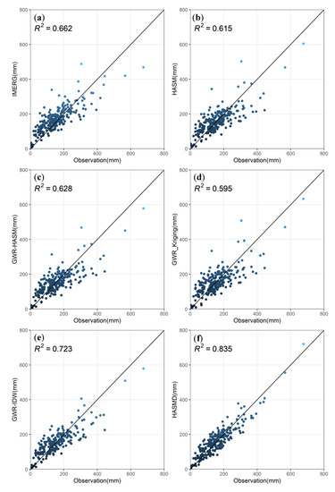
Figure 9.
Heatscatter plots of the validation between ground observations and the downscaling results in July: (a) the original IMERG product; (b) the HASM results; (c) the GWR-HASM results; (d) the GWR-Kriging results; (e) the GWR-IDW results; (f) the HASMD results.
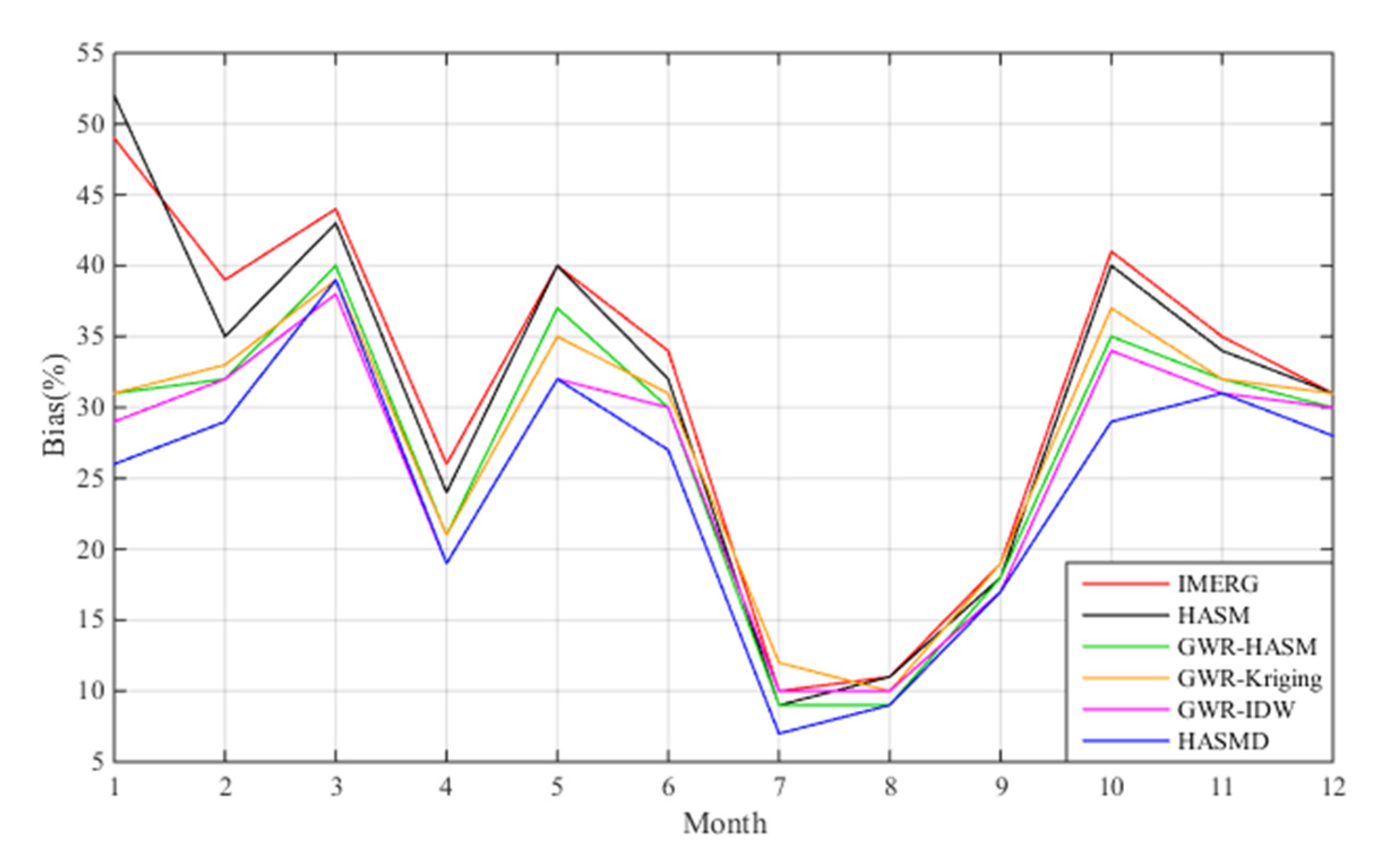
The downscaled results were further compared with the values obtained from the meteorological stations for the twelve months. Figure 10 displays the area mean bias values of IMERG, HASM, GWR-HASM, GWR-Kriging, GWR-IDW, and HASMD over mainland China. As can be seen from the figure, the prediction results of HASMD were closer to the true values than the prediction results of IMERG, HASM, GWR-HASM, GWR-Kriging, and GWR-IDW, with decreasing mean bias values of 22%, 19%, 10%, 13%, and 7%, respectively. Although the GWR-IDW method performed slightly better than HASMD in terms of bias in March, HASMD exhibited better performance than GWR-IDW in other months. Compared to the original IMERG products, the bias of HASMD decreased at rates of 8–47% for the twelve months, with mean decreasing rates of 19%, 24%, 16% and 28% in spring, summer, autumn and winter, respectively.
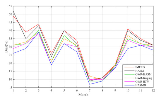
Figure 10.
Bias values obtained from different methods.
5. Discussion
Studies have shown that IMERG precipitation estimates perform well when compared with other satellite and reanalysis precipitation products in China [7,56,57]. The performance of the original IMERG products was spatially examined first at the monthly scale (Figure 5) in this study. Overestimations and underestimations were both observed, with maximum bias larger than 100 mm, 160 mm, 300 mm, and 130 mm for January, April, July and October, respectively. Downscaling is a potential method for obtaining precipitation estimates with high accuracy and high resolution. This study proposed a new downscaling method based on HASM, which was developed according to the differential geometry.
Previous studies related to HASM have mainly focused on the interpolation of different geographical variables. The good performance of HASM has been validated by researchers [26,28,29,30,31,32,33,34,35,36]. In this study, we proposed a new downscaling method, HASMD, based on HASM by introducing a new scale transformation equation. In addition, to obtain better downscaling precipitation estimations, the initial value of HASMD was set by applying GWR with the same auxiliary information as in GWR-based methods. We then compared HASMD with HASM, which was initialized by the results of a simple linear interpolator. The performance of the GWR-based downscaled methods, including GWR-Kriging, GWR-IDW and GWR-HASM, was also analyzed. The ordinary Kriging and IDW were performed using the module of 3D analyst ArcGIS 10.5. Different parameters for Kriging and IDW were compared and the best parameters for each technique with the smallest RMSE values were decided. For Kriging, the spherical semivariogram model with twenty samples provided the overall best result. The lowest RMSE value for IDW was found with a neighborhood of twelve points and power of two. The results showed that, compared with HASM, the accuracy of GWR-IDW and GWR-HASM improved by 11% and 9%, respectively, according to the RMSE values of the four months, and GWR-Kriging performed worse than HASM in July. Overall, the downscaled results obtained from HASMD outperformed the original IMERG products and the results of HASM, GWR-HASM, GWR-Kriging, and GWR-IDW, with mean decreasing rates of 26.5%, 19.2%, 11.3%, 16.8%, and 9.5%, respectively, in terms of the RMSE values. The underestimations and overestimations in the original IMERG products were modified by using HASMD, with the mean bias value decreasing by 22% over mainland China.
The performance of HASM is not stable, exhibiting relatively good performance in January compared with other months (Table 1). Moreover, from the spatial patterns of the downscaled precipitation (Figure 6b and Figure 8b), the HASM results showed high spatial heterogeneity, especially in July, with RMSE values larger than those of the original IMERG products. In Figure 6 and Figure 8, it can be seen that the results of GWR-based methods seem to be smoother than those of HASM and HASMD. Although the spatial patterns of precipitation obtained from the GWR-based methods mainly depend on the GWR method, the accuracy of them is determined by the combined methods of GWR and residual correction methods. In this study, we did not use many explanatory variables because studies have shown that the inclusion of more explanatory variables did not guarantee better results than those achieved using less variables [13]. The variables selected for the GWR method are based on correlation analysis from the global perspective, whereas the GWR method focuses on local modeling. Moreover, the GWR method is based on the assumption of independence and homogeneity of variance, which is difficult to satisfy in practice. As mentioned above, the initial value of HASMD is the result of the GWR method that uses the same explanatory variables as in GWR-based methods. Figure 7, Figure 9 and Figure 10 and Table 1 show that HASMD gives the best results, followed by GWR-IDW (Figure 10). This indicates that the scale transformation equation (Equation (4)) in HASMD, which integrates the spatial autocorrelation of the precipitation, plays a major role in the improvement of the final results.
Although HASMD is time consuming due to the solving of complex differential equations, this limitation could be resolved by realizing it in a parallel environment. The main limitation of HASMD lies in the downscaling of daily precipitation datasets since it is based on the second-order partial differential equations, which means that the estimated fields should be smooth. However, it is known that there exists strong spatial heterogeneity for the daily precipitation in China. Future studies could be conducted by introducing a regularity term in HASMD to downscale the satellite-based daily precipitation products.
6. Conclusions
The importance of precipitation downscaling is well recognized in hydrological studies and climate change fields. However, most statistical downscaling methods were established under some assumptions, which are highly data-dependent and not applicable for arbitrary regions. Recent developments in surface modeling methods based on differential geometry have brought new opportunities to provide new downscaling methods for enhancing the results. This study proposed a new downscaling method, HASMD, based on the good performance of HASM. A scale transformation equation was introduced in HASM, and its initial value was set by considering the explanatory variables of precipitation. Most studies focus on downscaling methods in local regions. However, the resolution of available precipitation products in large areas is relatively coarse at the present time. The developed downscaling method was thus applied to downscale the monthly IMERG products from a resolution of 0.1° to 0.01° in China. By comparing the results of HASMD with those of HASM, GWR-HASM, GWR-Kriging, and GWR-IDW, the high accuracy of HASMD was validated, which is capable of capturing the nonlinear spatial patterns of precipitation. Compared with the original IMERG precipitation products, the downscaling accuracy of HASMD was improved up to 47% in terms of RMSE. The proposed downscaling method provides a new way to obtain high accuracy and high spatial resolution remote sensing-based precipitation datasets. HAMSD is expected to show good performance in local areas, which will be investigated further. In addition, future studies could conduct sensitivity analysis on different timescales and consider the regularization of HASMD for downscaling satellite-based daily precipitation datasets.
Author Contributions
Conceptualization, N.Z.; methodology, N.Z. and Y.J.; software, Y.J.; validation, N.Z. and Y.J.; formal analysis, N.Z.; investigation, N.Z.; resources, Y.J.; data curation, Y.J.; writing—original draft preparation, N.Z.; writing—review and editing, N.Z. and Y.J.; visualization, N.Z. and Y.J.; supervision, N.Z.; project administration, N.Z.; funding acquisition, N.Z. All authors have read and agreed to the published version of the manuscript.
Funding
This research was funded by the National Natural Science Foundation of China (grant number 42071374, 41930647) and the Program of Frontier Sciences of Chinese Academy of Sciences, grant number ZDBS-LY-DQC005.
Data Availability Statement
The data are not publicly available due to the confidentiality of the research projects.
Acknowledgments
We thank the editor and the anonymous reviewers for their constructive comments and suggestions. We also acknowledge the technical support provided by Tianxiang Yue, Zhiru Ren and Zhengping Du.
Conflicts of Interest
The authors declare no conflict of interest.
References
- Donohoe, A. Atmospheric science: Energy and precipitation. Nat. Geosci. 2016, 9, 861. [Google Scholar] [CrossRef]
- Tuel, A.; Eltahir, E.A.B. Seasonal precipitation forecast over Morocco. Water Resour. Res. 2018, 54, 9118–9130. [Google Scholar] [CrossRef]
- Casellas, E.; Bech, J.; Veciana, R.; Pineda, N.; Rigo, T.; Miro, J.R.; Sairouni, A. Surface precipitation phase discrimination in complex terrain. J. Hydrol. 2021, 592, 125780. [Google Scholar] [CrossRef]
- Hou, A.Y.; Kakar, R.K.; Neeck, S.; Azarbarzin, A.A.; Kummerow, C.D.; Kojima, M.; Oki, R.; Nakamura, K.; Iguchi, T. The global precipitation measurement mission. Bull. Am. Meteorol. Soc. 2014, 95, 701–722. [Google Scholar] [CrossRef]
- Skofronick-Jackson, G.; Petersen, W.A.; Berg, W.; Kidd, C.; Stocker, E.F.; Kirschbaum, D.B.; Kakar, R.; Braun, S.A.; Huffman, G.J.; Iguchi, T.; et al. The global precipitation measurement (GPM) mission for science and society. Bull. Am. Meteorol. Soc. 2017, 98, 1679–1695. [Google Scholar] [CrossRef]
- Chen, C.; Chen, Q.; Duan, Z.; Zhang, J.; Mo, K.; Li, Z.; Tang, G. Multiscale comparative evaluation of the GPM IMERG v5 and TRMM 3B42 v7 precipitation products from 2015 to 2017 over a climate transition area of China. Remote Sens. 2018, 10, 944. [Google Scholar] [CrossRef] [Green Version]
- Tang, G.; Clark, M.P.; Papalexiou, S.M.; Ma, Z.; Hong, Y. Have satellite precipitation products improved over last two decades? A comprehensive comparison of GPM IMERG with nine satellite and reanalysis datasets. Remote Sens. Environ. 2020, 240, 111697. [Google Scholar] [CrossRef]
- Tan, J.; Petersen, W.A.; Tokay, A. A novel approach to identify sources of errors in IMERG for GPM ground validation. J. Hydrometeorol. 2016, 17, 2477–2491. [Google Scholar] [CrossRef]
- Mahmoud, M.T.; Mohammed, S.A.; Hamouda, M.A.; Mohamed, M.M. Impact of topography and rainfall intensity on the accuracy of IMERG precipitation estimates in an arid region. Remote Sens. 2020, 13, 13. [Google Scholar] [CrossRef]
- Sharifi, E.; Saghafian, B.; Steinacker, R. Downscaling satellite precipitation estimates with multiple linear regression, artificial neural networks, and spline interpolation techniques. J. Geophys. Res. Atmos. 2019, 124, 789–805. [Google Scholar] [CrossRef] [Green Version]
- Zhao, N.; Yue, T.; Chen, C.; Zhao, M.; Fan, Z. An improved statistical downscaling scheme of tropical rainfall measuring mission precipitation in the Heihe River basin, China. Int. J. Climatol. 2018, 38, 3309–3322. [Google Scholar] [CrossRef]
- Chaudhuri, C.; Robertson, C. CliGAN: A structurally sensitive convolutional neural network model for statistical downscaling of precipitation from multi-model ensembles. Water 2020, 12, 3353. [Google Scholar] [CrossRef]
- Lu, X.Y.; Tang, G.Q.; Wang, X.Q.; Liu, Y.; Wei, M.; Zhang, Y.X. The development of a two-step merging and downscaling method for satellite precipitation products. Remote Sens. 2020, 12, 398. [Google Scholar] [CrossRef] [Green Version]
- Sachindra, D.A.; Perera, B.J. Statistical downscaling of general circulation model outputs to precipitation accounting for non-stationarities in predictor-predictand relationships. PLoS ONE 2016, 11, e0168701. [Google Scholar]
- Xu, M.; Liu, Q.; Sha, D.; Yu, M.; Duffy, D.Q.; Putman, W.M.; Carroll, M.; Lee, T.; Yang, C. PreciPatch: A dictionary-based precipitation downscaling method. Remote Sens. 2020, 12, 1030. [Google Scholar] [CrossRef] [Green Version]
- Jing, W.; Yang, Y.; Yue, X.; Zhao, X. A comparison of different regression algorithms for downscaling monthly satellite-based precipitation over North China. Remote Sens. 2016, 8, 835. [Google Scholar] [CrossRef] [Green Version]
- Chaudhuri, C.; Srivastava, R. A novel approach for statistical downscaling of future precipitation over the Indo-Gangetic Basin. J. Hydrol. 2017, 547, 21–38. [Google Scholar] [CrossRef]
- Shamir, E.; Halper, E.; Modrick, T.; Georgakakos, K.P.; Chang, H.-I.; Lahmers, T.M.; Castro, C. Statistical and dynamical downscaling impact on projected hydrologic assessment in arid environment: A case study from Bill Williams River basin and Alamo Lake, Arizona. J. Hydrol. 2019, 2, 100019. [Google Scholar] [CrossRef]
- Sachindra, D.A.; Ahmed, K.; Rashid, M.M.; Shahid, S.; Perera, B.J.C. Statistical downscaling of precipitation using machine learning techniques. Atmos. Res. 2018, 212, 240–258. [Google Scholar] [CrossRef]
- Jing, W.; Yang, Y.; Yue, X.; Zhao, X. A spatial downscaling algorithm for satellite-based precipitation over the Tibetan Plateau based on NDVI, DEM, and land surface temperature. Remote Sens. 2016, 8, 655. [Google Scholar] [CrossRef] [Green Version]
- Seyoum, W.; Kwon, D.; Milewski, A. Downscaling GRACE TWSA data into high-resolution groundwater level anomaly using machine learning-based models in a glacial aquifer System. Remote Sens. 2019, 11, 824. [Google Scholar] [CrossRef] [Green Version]
- Baez-Villanueva, O.M.; Zambrano-Bigiarini, M.; Beck, H.E.; McNamara, I.; Ribbe, L.; Nauditt, A.; Birkel, C.; Verbist, K.; Giraldo-Osorio, J.D.; Xuan Thinh, N. RF-MEP: A novel random forest method for merging gridded precipitation products and ground-based measurements. Remote Sens. Environ. 2020, 239, 111606. [Google Scholar] [CrossRef]
- Yuan, Q.; Shen, H.; Li, T.; Li, Z.; Li, S.; Jiang, Y.; Xu, H.; Tan, W.; Yang, Q.; Wang, J. Deep learning in environmental remote sensing: Achievements and challenges. Remote Sens. Environ. 2020, 241, 111716. [Google Scholar] [CrossRef]
- Qu, Y.; Zhu, Z.; Montzka, C.; Chai, L.; Liu, S.; Ge, Y.; Liu, J.; Lu, Z.; He, X.; Zheng, J. Inter-comparison of several soil moisture downscaling methods over the Qinghai-Tibet Plateau, China. J. Hydrol. 2021, 592, 125616. [Google Scholar] [CrossRef]
- Stott, J.P. Review of Surface Modeling. In Proceedings of the Surface Modeling by Computer, a Conference Jointly Sponsored by the Royal Institution of Chartered Surveyors and the Institition of Civil Engineers, London, UK, 6 October 1976; pp. 1–8. [Google Scholar]
- Yue, T.X. Surface Modeling: High Accuracy and High Speed Methods; CRC Press: New York, NY, USA, 2011. [Google Scholar]
- Hestenes, M.R.; Stiefel, E.F. Methods of conjugate gradients for solving linear systems. J. Res. Nat. Bur. Stand. 1952, 49, 409–436. [Google Scholar] [CrossRef]
- Thompson, J.F.; Thames, F.C.; Mastin, C.W. Automatic numerical generation of body-fitted curvilinear coordinate system for field containing any number of arbitrary two-dimensional bodies. J. Comput. Phys. 1974, 15, 299–319. [Google Scholar] [CrossRef]
- Chen, C.F.; Yue, T.X. A method of DEM construction and related error analysis. Comput. Geosci. 2010, 36, 717–725. [Google Scholar] [CrossRef]
- Chen, C.F.; Yue, T.X.; Dai, H.; Tian, M.Y. The smoothness of HASM. Int. J. Geogr. Inf. Sci. 2013, 27, 1651–1667. [Google Scholar] [CrossRef]
- Shi, W.J.; Yue, T.X.; Du, Z.P.; Wang, Z.; Li, X.W. Surface modeling of soil antibiotics. Sci. Total Environ. 2016, 543, 609–619. [Google Scholar] [CrossRef]
- Shi, W.; Liu, J.; Du, Z.; Song, Y.; Chen, C.; Yue, T. Surface modelling of soil pH. Geoderma 2009, 150, 113–119. [Google Scholar] [CrossRef]
- Zhao, N.; Yue, T.X. A modification of HASM for interpolating precipitation in China. Theor. Appl. Climatol. 2013, 116, 273–285. [Google Scholar] [CrossRef]
- Zhao, N.; Lu, N.; Chen, C.F.; Li, H.; Yue, T.X.; Zhang, L.L.; Liu, Y. Mapping temperature using a Bayesian statistical method and a high accuracy surface modelling method in the Beijing-Tianjin-Hebei region, China. Meteorol. Appl. 2017, 24, 571–579. [Google Scholar] [CrossRef] [Green Version]
- Zhao, N.; Yue, T.X.; Zhou, X.; Zhao, M.W.; Liu, Y.; Du, Z.P.; Zhang, L.L. Statistical downscaling of precipitation using local regression and high accuracy surface modeling method. Theor. Appl. Climatol. 2016, 129, 281–292. [Google Scholar] [CrossRef]
- Yue, T.X.; Zhao, N.; Fan, Z.M.; Li, J.; Chen, C.F.; Lu, Y.M.; Wang, C.L.; Gao, J.; Xu, B.; Jiao, Y.M.; et al. Methods for simulating climate scenarios with improved spatiotemporal specificity and less uncertainty. Glob. Planet. Chang. 2019, 181, 102973. [Google Scholar] [CrossRef]
- Wang, X.L.; Wen, Q.H.; Wu, Y. Penalized maximal t test for detecting undocumented mean change in climate data series. J. Appl. Meteorol. Climatol. 2007, 46, 916–931. [Google Scholar] [CrossRef]
- Huffman, G.J.; Kirschbaum, D.B.; Adler, R.F.; Braun, S.; Garrett, K.; Jones, E.; McNally, A.; Skofronick-Jackson, G.; Stocker, E.; Wu, H.; et al. NASA’s remotely sensed precipitation: A reservoir for applications users. Bull. Am. Meteorol. Soc. 2017, 98, 1169–1184. [Google Scholar]
- Huffman, G.J.; Bolvin, D.T.; Nelkin, E.J.; Tan, J. Integrated multi-satellitE retrievals for GPM (IMERG) technical documentation. NASA GSFC Code 2019, 612, 1–25. [Google Scholar]
- Somasundaram, D. Differential Geometry; Alpha Science International Ltd.: Harrow, UK, 2005. [Google Scholar]
- Henderson, D.W. Differential Geometry; Prentice-Hall Inc.: London, UK, 1998. [Google Scholar]
- Liseikin, V.D. A Computational Differential Geometry Approach to Grid Generation; Springer: Berlin/Heidelberg, Germany, 2004. [Google Scholar]
- Toponogov, V.A. Differential Geometry of Curves and Surfaces; Birkhaeuser Boston: New York, NY, USA, 2006. [Google Scholar]
- Golub, H.H.; O’Leary, D.P. Some history of the conjugate gradient and Lanczos algorithms: 1948–1976. SIAM Rev. 1989, 31, 50–102. [Google Scholar] [CrossRef]
- Van der Vorst, H.A. Efficient and reliable iterative methods for linear systems. J. Comput. Appl. Math. 2002, 149, 251–265. [Google Scholar] [CrossRef] [Green Version]
- Paige, C.C.; Saunders, M.A. LSQR: An algorithm for sparse linear euqations and sparse least squares. ACM Trans. Math. Softw. 1982, 8, 43–71. [Google Scholar] [CrossRef]
- Ford, W. Krylov subspace methods. Numer. Linear Algebr. 2015, 491–532. [Google Scholar] [CrossRef]
- Yilmaz, K.K.; Derin, Y. Evaluation of multiple satellite-based precipitation products over complex topography. J. Hydrometeorol. 2014, 15, 1498–1516. [Google Scholar]
- Zhang, T.; Li, B.; Yuan, Y.; Gao, X.; Sun, Q.; Xu, L.; Jiang, Y. Spatial downscaling of TRMM precipitation data considering the impacts of macro-geographical factors and local elevation in the Three-River Headwaters region. Remote Sens. Environ. 2018, 215, 109–127. [Google Scholar] [CrossRef]
- Hunink, J.E.; Immerzeel, W.W.; Droogers, P. A high-resolution precipitation 2-step mapping procedure (HiP2P): Development and application to a tropical mountainous area. Remote Sens. Environ. 2014, 140, 179–188. [Google Scholar] [CrossRef]
- Manz, B.; Buytaert, W.; Zulkafli, Z.; Lavado, W.; Willems, B.; Robles, L.A.; Rodríguez-Sánchez, J.P. High-resolution satellite-gauge merged precipitation climatologies of the Tropical Andes. J. Geophys. Res. Atmos. 2016, 121, 1190–1207. [Google Scholar] [CrossRef] [Green Version]
- Liu, J.; Zhang, W.; Nie, N. Spatial downscaling of TRMM precipitation data using an optimal subset regression model with NDVI and terrain factors in the Yarlung Zangbo River basin, China. Adv. Meteorol. 2018, 2018, 1–13. [Google Scholar] [CrossRef]
- Elnashar, A.; Zeng, H.; Wu, B.; Zhang, N.; Tian, F.; Zhang, M.; Zhu, W.; Yan, N.; Chen, Z.; Sun, Z.; et al. Downscaling TRMM monthly precipitation using Google Earth Engine and Google Cloud computing. Remote Sens. 2020, 12, 3860. [Google Scholar] [CrossRef]
- Stauffer, R.; Mayr, G.J.; Messner, J.W.; Umlauf, N.; Zeileis, A. Spatio-temporal precpitation climatology over complex terrain using a censored additive regression model. Int. J. Climatol. 2016, 37, 3264–3275. [Google Scholar] [CrossRef] [Green Version]
- Li, Y.; Wang, Q.J.; He, H.; Wu, Z.Y.; Lu, G.H. A method to extend temporal coverage of high quality precipitation datasets by calibrating reanalysis estimates. J. Hydrol. 2020, 581, 124355. [Google Scholar] [CrossRef]
- Dezfuli, A.K.; Ichoku, C.M.; Huffman, G.J.; Mohr, K.I.; Selker, J.S.; van de Giesen, N.; Hochreutener, R.; Annor, F.O. Validation of IMERG precipitation in Africa. J. Hydrometeorol. 2017, 18, 2817–2825. [Google Scholar] [CrossRef]
- Wang, S.M.; Wang, D.K.; Huang, C. Evaluating the applicability of GPM satellite precipitation data in Heihe River Basin. J. Nat. Res. 2018, 33, 1847–1860. [Google Scholar]


Publisher’s Note: MDPI stays neutral with regard to jurisdictional claims in published maps and institutional affiliations. |
© 2021 by the authors. Licensee MDPI, Basel, Switzerland. This article is an open access article distributed under the terms and conditions of the Creative Commons Attribution (CC BY) license (https://creativecommons.org/licenses/by/4.0/).