Article

Assessment of the Spatial and Temporal Patterns of Cover Crops Using Remote Sensing

1
Department of Food, Agricultural and Biological Engineering, The Ohio State University, Columbus, OH 43210, USA
2
School of Environment and Natural Resources, The Ohio State University, Wooster, OH 44691, USA
3
Ohio State University Extension, The Ohio State University, Fremont, OH 43420, USA
*
Author to whom correspondence should be addressed.
Remote Sens. 2021, 13(14), 2689; https://doi.org/10.3390/rs13142689
Submission received: 1 June 2021 / Revised: 4 July 2021 / Accepted: 6 July 2021 / Published: 8 July 2021
(This article belongs to the Special Issue Remote Sensing and Vegetation Mapping)

Abstract

:
Cover cropping is a conservation practice that helps to alleviate soil health problems and reduce nutrient losses. Understanding the spatial variability in historic and current adoption of cover cropping practices and their impacts on soil, water, and nutrient dynamics at a landscape scale is an important step in determining and prioritizing areas in a watershed to effectively utilize this practice. However, such data are lacking. Our objective was to develop a spatial and temporal inventory of winter cover cropping practices in the Maumee River watershed using images collected by Landsat satellites (Landsat 5, 7 and 8) from 2008 to 2019 in Google Earth Engine (GEE) platform. Each year, satellite images collected during cover crop growing season (i.e., between October and April) were converted into two seasonal composites based on cover crop phenology. Using these composites, various image-based covariates were extracted for 628 ground-truth (field) data. By integrating ground-truth and image-based covariates, a cover crop classification model based on a random forest (RF) algorithm was developed, trained and validated in GEE platform. Our classification scheme differentiated four cover crop categories: Winter Hardy, Winter Kill, Spring Emergent, and No Cover. The overall classification accuracy was 75%, with a kappa coefficient of 0.63. The results showed that more than 50% of the corn-soybean areas in the Maumee River watershed were without winter crops during 2008–2019 period. It was found that 2019/2020 and 2009/2010 were the years with the largest and lowest cover crop areas, with 34% and 10% in the watershed, respectively. The total cover cropping area was then assessed in relation to fall precipitation and cumulative growing degree days (GDD). There was no apparent increasing trend in cover crop areas between 2008 and 2019, but the variability in cover crops areas was found to be related to higher accumulated GDD and fall precipitation. A detailed understanding of the spatial and temporal distribution of cover crops using GEE could help in promoting site-specific management practices to enhance their environmental benefits. This also has significance to policy makers and funding agencies as they could use the information to localize areas in need of interventions for supporting adoption of cover cropping practice.

Graphical Abstract

1. Introduction

There is a growing concern that some conventional agricultural practices lead to the degradation of soil health properties and contribute to water quality problems over time. Cover cropping has been recommended as one of the conservation practices suitable for addressing these problems while improving crop productivity and farm profitability [1,2]. By reducing soil compaction, fixing nitrogen in soil, enhancing soil organic matter and reducing nutrient losses through soil erosion and surface runoffs [3,4,5,6], it helps improve soil health and water quality. It also provides several other ecosystem services, including reduction in greenhouse gas emission, weed control, and biodiversity enhancement [7,8,9].
Cover crops are usually planted after or closer to harvest of spring cash crops in various forms, including grass, legume, brassica, or a mixture of grass and legume, and terminated before planting of next year’s cash crops. Although they are not new to US agricultural system, their adoption is relatively limited [10]. Farmers are concerned about incorporating cover crops into their crop rotations due to timing and economic issues related to establishment and termination of cover crops, required management changes such as tillage or nutrient application, as well as potential negative impacts on water balance and yields of cash crops such as corn and soybean [11]. As such, several state and federal funding programs, including the NRCS Environmental Quality Incentives Program (EQIP) and the Conservation Stewardship Program (CSP), have been focused on promoting their adoption. Despite significant increases in state and federal incentives to promote farmers’ participation in cover crop programs, there lacks a clear understanding of where these investments are making a major impact. Currently, surveys are being used as a major approach to examine the adoption and impacts of cover crops. Surveys however provide an incomplete and often biased representation of the overall practices on the ground. For instance, a 2019–2020 survey of cover crops was based on 1172 farmers across the US [12]. Additionally, surveys are time-consuming, labor intensive and cost prohibitive to scale-up to larger areas.
Unlike surveys, remote sensing, particularly satellite data, offers a promising approach to cost-effectively and timely detection and monitoring of cover crop use and growth at a higher temporal and spatial scale across landscapes. This capability has recently been bolstered by the availability of a large volume of freely available data from frequently revisiting medium-resolution satellites such as Landsat (30 m) and Sentinel (10 m). Since green and healthy vegetations have higher reflectance in near-infrared (NIR) than other spectral regions, prior studies have leveraged visible and NIR (VIS NIR) satellite imagery to understand, classify and monitor winter cover crops at a landscape scale [13,14,15,16,17]. For instance, Hively et al. [17] assessed cover crop areas in Chesapeake Bay watershed in southeastern Pennsylvania between 2010 and 2013 using one image per winter collected from Landsat and SPOT satellites. Similarly, Rundquist & Carlson [10] used normalized difference vegetation index (NDVI) derived from Landsat-7 and Landsat-8 satellite images, collected during winter to identify cover cropped fields in Illinois, Indiana, and Iowa. Since the growing season of cover crops is between fall and spring, use of only a single image to understand and classify cover crops represents some limitations of these prior studies.
To address some of these issues, Seifert et al. [15] used the concept of seasonal composites of satellite images, collected from multiple Landsat missions (Landsat 5, 7, and 8) during the cover crop growing season (i.e., October to April) to map cover crop areas in the eight midwestern states from 2008 to 2016. For each cover crop season, the study used a single composite of satellite data. A single seasonal composite averages out spectral reflectance of crops over a growing season. While this helps to broadly classify whether a field is planted with cover crops or not, it is difficult to account for temporal variability in cover crop phenology. Such single seasonal composites have limited use when it comes to understanding cover crop performance, including timing of their establishment and growth, which are often influenced by weather, management practices, and field conditions. Considering these limitations, Hagen et al. [13] used a time series of NDVI data from November through July every year between 2005 to 2018 to estimate five major cover crop categories (i.e., winter kill, full cover, spring emergent, winter wheat, and not covered) in the midwestern United States. This study compared timing and intensity of cover crops’ greenness with NDVI thresholds set at the HUC8 scale to determine cover crop categories. The NDVI thresholds were estimated based on analyses of handful ground-truth data in relation to satellite imagery. The study highlighted the importance of multiple data points per growing season to assess temporal variability of crop cover and growth on the croplands.
Use of historic satellite images to identify trends and changes in crop growth can be computationally intensive if a study area is large and conventional mapping approaches (e.g., image download and their processing at desktop(s)) are adopted. For instance, a single uncompressed Landsat 8 scene is larger than 1.6 gigabytes, and thus, the applications involving multiple scenes require computing resources, which can present challenges to many practitioners [18]. To overcome some of these challenges, cloud-based platforms, most notably Google Earth Engine (GEE), has emerged, providing the scientific community an unprecedented volume of ready-to-use satellite data, including the entire Landsat archive, as well as state-of-the-art data analytics for rapid and seamless processing [19]. By storing and processing images on numerous remote servers, GEE removes the need to download and process data on local stand-alone computers [19].
To date, several studies have explored and demonstrated the utility of GEE for mapping agricultural practices and vegetation health at regional [20,21,22] and global scales [23,24], with only a few studies [15] using GEE for mapping cover crop practices. The aim of this study is to develop a comprehensive and scalable mapping approach, and assess spatial and temporal patterns of cover crops in GEE focusing mainly on corn and soybean fields. The methodology was developed based on a thorough review of cover crop remote sensing literature and incorporates the best available practices. Additionally, the spatial and temporal patterns of cover crop growth were evaluated in relation to precipitation and temperature at a landscape scale—a newer perspective that was less explored in prior works. The developed GEE modeling framework was tested on the Maumee River watershed (MRW), which is the largest watershed in the Western Lake Erie basin (WLEB) and one of the most impaired basins in the U.S. Specifically, we integrated historical satellite time series data with ground truth observations in the GEE platform to develop cover crop inventory between 2008 and 2019.

2. Materials and Methods

The MRW is a highly productive and intensively managed agricultural region of Indiana, Michigan and Ohio, where about 80% of the land is in corn and soybean production (Figure 1). Intensive management practices associated with corn and soybean production [25,26] in this region have been found to be the primary source of nitrogen and phosphorous loads to the Maumee River [27,28,29], which drains to Lake Erie. The increase in nutrient concentrations has contributed to increasing occurrences of harmful algal blooms in Lake Erie, posing a serious threat to aquatic and human health. As such, an increasing emphasis has been placed on adoption of conservation practices including cover crops [5].

2.1. Data

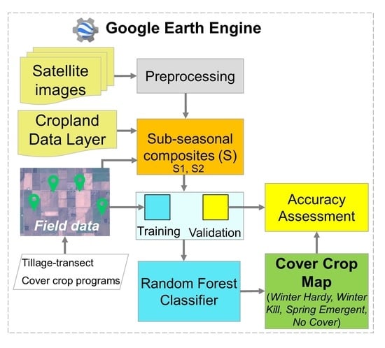
2.1.1. Satellite Data Acquisition and Preprocessing

Satellite images from Landsat 5, 7 and 8 with less than 50% cloud cover, covering northern and northwest part of Ohio were collected for each cover crop growing season (i.e., October to April) during 2008 to 2019. Selection of images from various Landsat missions was based on their lifespans and data availability (Table 1). GEE, a cloud-based platform developed and made publicly available by Google [19], was used to facilitate easier and faster preprocessing and analyses of these satellite images. Specifically, a JavaScript-based Earth Engine Code Editor was used to access and prepare Level-2 surface reflectance (SR) products from Landsat, and SR products are corrected for atmospheric attenuation and disturbances on each individual scene. To get rid of unwanted image pixels contaminated by cloud, cloud shadow and snow, and provide accurate representation of vegetation health, a Quality Assessment (QA) band generated through a CFMask algorithm [30] was used for all the Landsat scenes.
While all the images were from the same Landsat satellite system, there existed slight differences in spectral signatures of an object across images from three Landsat missions. For instance, for both soil surfaces and vegetations, Roy et al. [33] observed higher NDVI based on ETM+ images than that of OLI images. To ensure these differences were resolved for long-term time series analyses, Roy et al. [33] developed spectral transformation functions between OLI and TM/ETM+ data by fitting an ordinary least squares (OLS) regression with r2 > 0.7 for reflectance and >0.9 for NDVI. The slopes and intercepts of the regression models corresponding to each individual band are shown in the Equations (1) and (2). Using these spectral transformation functions developed by Roy et al. [33], TM and ETM+ based images were transformed into OLI spectral space. This process is also called harmonization, which has been found to be useful in eliminating several issues that are part of satellite data such as missing data due to SLC off, cloud cover, and shadow removal [34,35].
I n t e r c e p t = [ 0.0003 ,   0.0088 ,   0.0061 ,   0.0412 ,   0.0254 ,   0.0172 ]
for (Blue, Green, Red, NIR, SWIR1, SWIR2)
S l o p e s = [ 0.8474 ,   0.8483 ,   0.9047 ,   0.8462 ,   0.8937 ,   0.9071 ]
for (Blue, Green, Red, NIR, SWIR1, SWIR2)

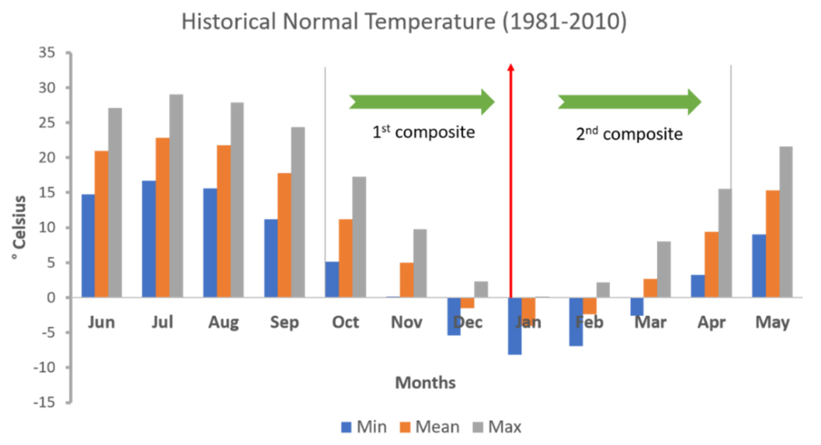
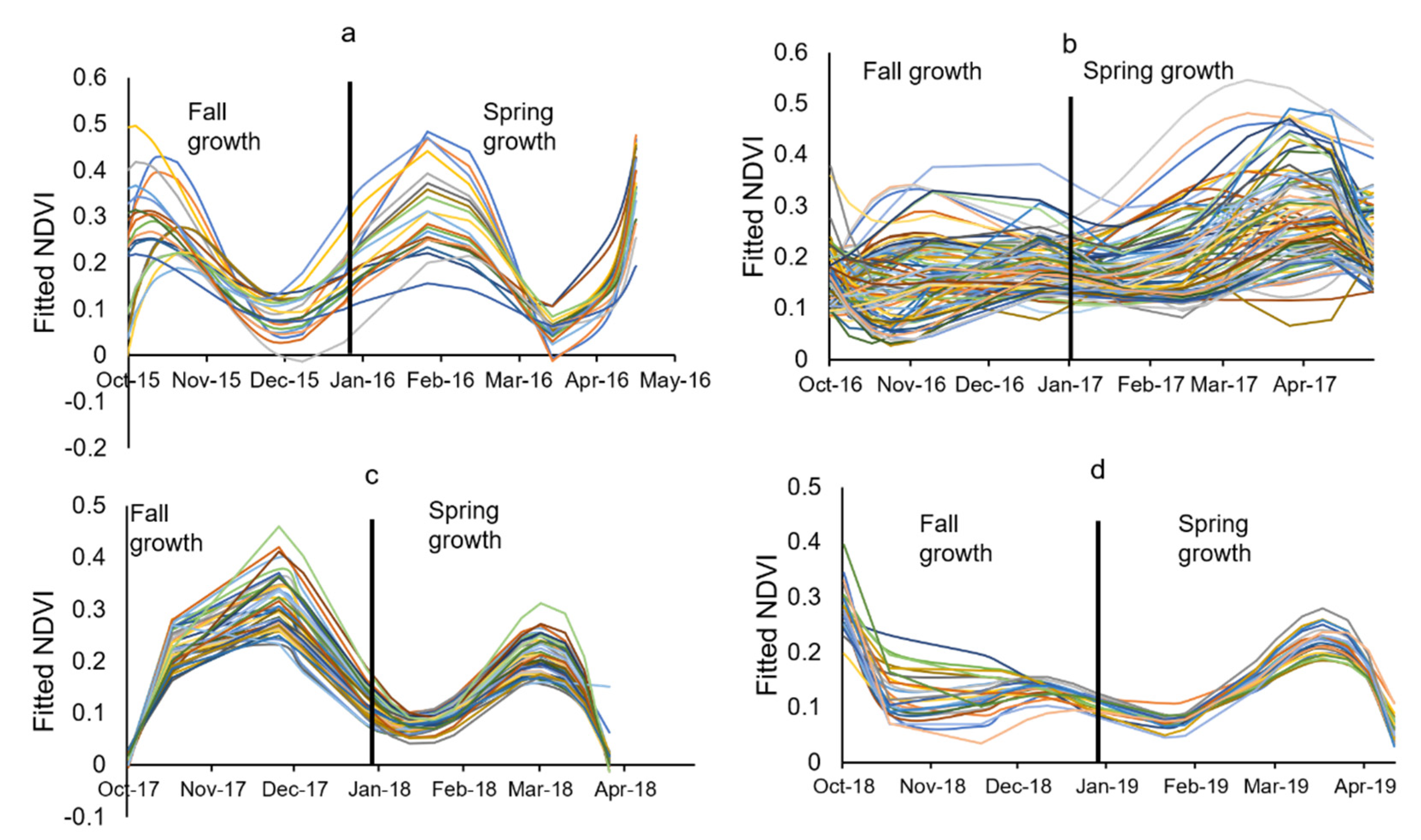
2.1.2. Harmonic Analyses and Seasonal Composites

Since the MRW is a big region, it was difficult to find a series of individual image scenes with cloud cover less than 50% covering the same geographic extent across multiple dates within the growing season. To capture crop phenology through analyses of multidate images, we implemented a concept of seasonal composites by considering median of satellite images collected during a given cover crop growing season [22,36,37,38]. To determine the number of seasonal composites suitable for monitoring cover crops’ growth, it is critical to understand their growing season. As such, historical (1981 to 2010) weather pattens across the MRW were assessed using the temperature data available from the PRISM Climate Group [39]. Typically, in MRW, the month of December marks the start of cold winter, when cover crops are either killed by frost or stay dormant (Figure 2) [40]. It was assumed that while some cover crops get terminated before winter or naturally die, some that are unable to grow properly or emerge during fall months could grow or emerge in the spring with warming of the weather.
A harmonic analysis (also known as Fourier transformation) was applied on Landsat 8-derived NDVI data to analyze and characterize the underlying seasonal phenology of cover crops in the study region [41]. For this, average NDVI was computed by considering all the pixels within boundaries for all the ground-truth cover crop fields that were collected between 2015/2016 and 2018/2019 from Erie and Huron counties (discussed in detail in the Section 2.1.4 below) (Figure 1). Fourier series/transform models any time series data as a combination of sine and cosine curves parameterized by amplitude/phase as well as distribution of frequency [42]. Addition of successive harmonics in the transformation brings the curve closer to the original curve. Similar to prior works [43,44], Fourier transformation of NDVI data suggested that cover crops in the study region follow a bimodal pattern; the amplitude of second order harmonic was dominant for about 73% of the total fields considered (Figure 3).
To capture these two major seasonal variabilities in cover crop growth, two composites were prepared, the first based on satellite images collected between October and December, and second based on images between January and April (Figure 3). These composites were then masked using annual Cropland Data Layer (CDL) at 30 m resolution created by the National Agricultural Statistics Service (NASS), USDA [45] which is available in the GEE platform. In addition to estimating median values per pixels for each individual spectral band (Table 2), several commonly and widely used vegetation indices (VIs), such as NDVI [15,38,44,46,47,48], Difference Vegetation Index (DVI), Normalized Green Red Difference Index (NGRDI) [49] and Ratio Vegetation Index (RVI) [50] were created and added to the composites. Similarly, composites representing minimum and maximum NDVI values were created and added due to their proven importance in mapping of crops [15,51]. For this, the pixel-based reducer function in GEE was used. As such, each composite consisted of 12 bands (Table 2), with each band representing a feature that is potentially useful in understanding crops’ properties in a season.

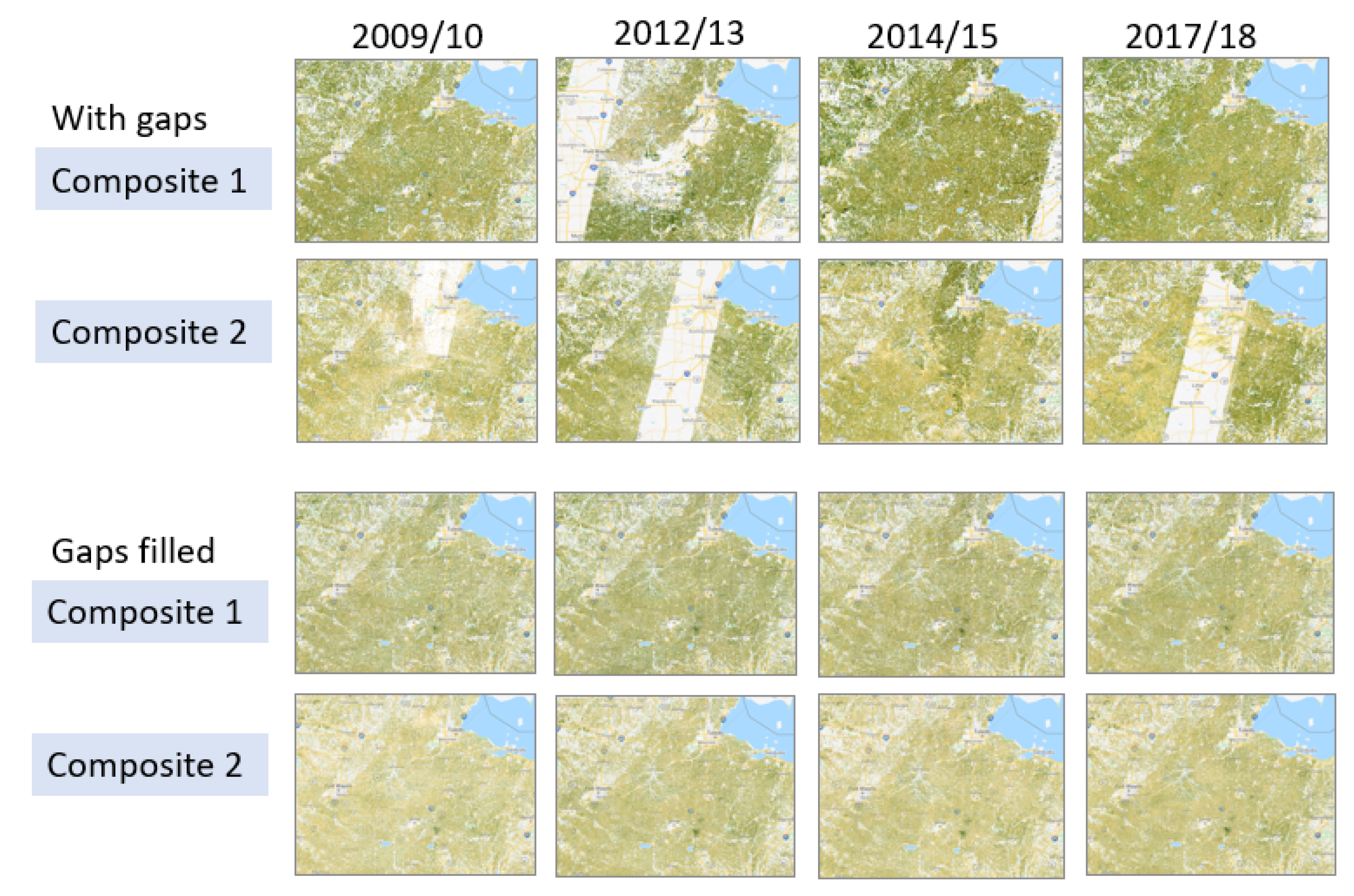
2.1.3. Filling in Data Gaps in Seasonal Composites
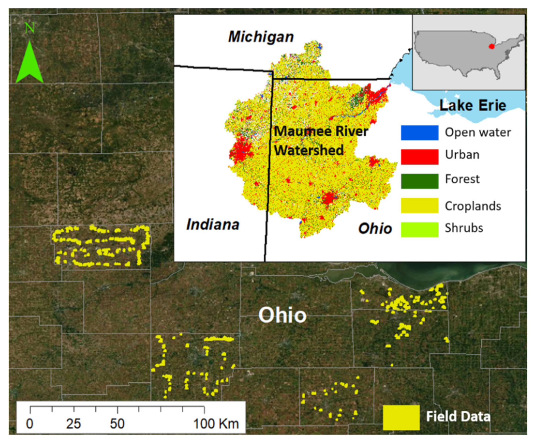
Despite temporal aggregation of satellite images, some data gaps were observed in seasonal composites such as a first composite for 2012/2013, and second composites for 2009/2010, 2012/2013, 2014/2015, 2017/2018. This was mainly due to 16 days temporal resolution of Landsat satellite data in combination with consistent cloud and snow cover. To address this concern, we used 16-day Landsat and daily MODIS fused monthly images produced using the Highly Scalable Temporal Adaptive Reflectance Fusion Model (HISTARFM) algorithm [52] (Figure 4). Although there exist some differences between the wavelength range covered by the derived HISTARFM and Landsat band reflectance, they were found to be highly correlated (0.85–0.92) [52] which provides a strong basis for its use in applications such as this.

2.1.4. Field Data

A total of 628 cover crop fields recorded in a cropland roadside transect survey across five counties in Northern Ohio were used as ground-truth data. The transect survey was designed to collect data on tillage and crop residue management systems across the targeted counties [53]. The fields that were clearly visible from the roadside, planted in a relatively short period of time and which were adopted on conservation tillage were most likely to be selected for the transect survey. The field selections primarily relied upon the sampling of county road as the routes for roadside survey were first established considering multiple criteria such as avoiding large urbanized areas, forested land, rangeland and highways. Information about 255 fields was gathered between 2015 to 2018 based on the Cover Crop Aggregation Program, which was digitized using transect survey data from Erie and Huron counties. An additional 373 records were based on digitized transect surveys in Fulton, Hancock, and Crawford counties from 2015 to 2019. While only Fulton and Hancock counties lie in the MRW, the data from Crawford, Erie and Huron county were used to enrich the limited ground-truth data. For each winter season, there were different numbers of cover crop fields (Table 3). Since the information about these fields were available in a point format (i.e., latitude and longitude), boundaries for these fields were digitized. To avoid mixed pixels (i.e., ensuring only pixels from within a field are included) during extraction of image information [15], field boundaries were buffered inward by 30 m (equals to the Landsat resolution). It is important to note that although these fields were observed to have ground covers during the time of surveys, it does not necessarily mean that these fields had good cover throughout the season because extent of ground cover can be influenced by weather, field conditions and management practices.
To analyze the growth pattern of cover crops, a threshold of 0.3 was applied on an average NDVI estimated for each cover crop field. In previous studies [16,17], a NDVI value higher than 0.3 provided an indication for a higher vegetation cover of winter crops. Using this threshold, the fields were grouped and labelled into four categories: Winter Hardy (significant growth in fall and spring), Winter Kill (significant growth only in fall), Spring Emergent (significant growth in spring), and Not Covered (no significant growth in both periods) based on their average NDVI over fall and spring.
For classification of cover crops, a pixel-based approach was used. To prepare datasets for classification, the ground-truth fields were randomly split into training (60%) and validation (40%) groups. Pixels within a field are often spatially autocorrelated, so the inclusion of pixels from a field into both training and test dataset can often lead to overestimation of classification accuracy [15,36]. To avoid concerns related to spatial autocorrelation, pixels representing these fields were split into training and testing dataset, ensuring that the pixels from a field are included either in training or testing dataset but not both. For each field in training and validation group, pixel values were extracted from the corresponding year’s image composites and this resulted in 38,632 pixels for training and 30,124 pixels for validation.

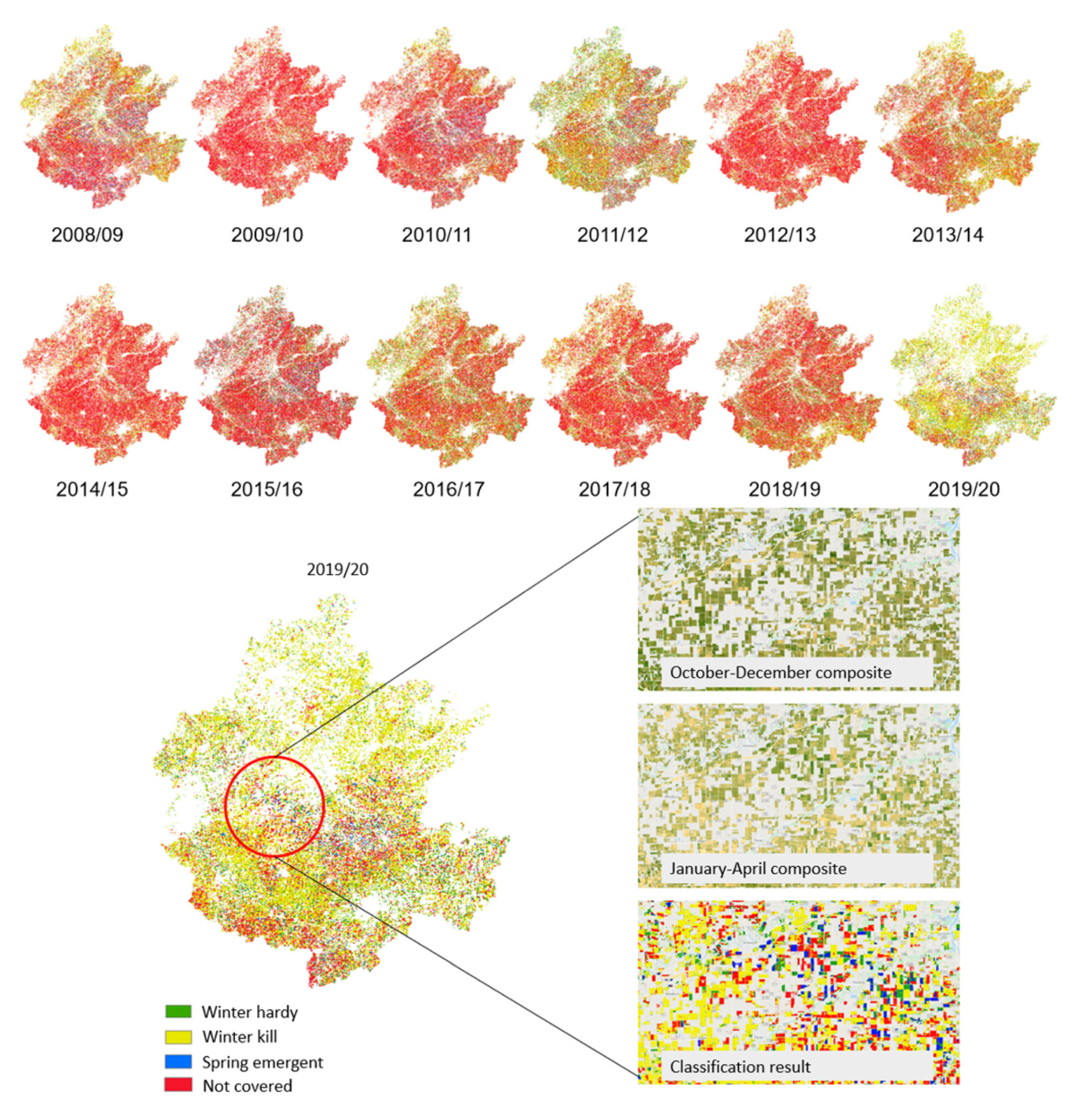
2.2. Cover Crop Classification

A random forest (RF) algorithm, one of the most widely applied algorithms in remote sensing community in recent years [54,55,56,57], was used to classify the image composites into four cover crop categories. RF has been found to consistently outperform other classification algorithms, particularly for applications related to crop classifications [58,59,60]. Since it is an ensemble of individual uncorrelated decision trees, created from the random bootstrap samples that use randomly selected subset of features [61], it is robust against noise and overfitting and able to handle high dimensional data [62,63]. The final output of this algorithm is calculated by aggregating outputs from all the decision trees. While a majority voting is used for classification, an average of outputs from various decisions trees is used for regression. It implements the bagging technique to make final prediction from multiple decision trees, which are based on bootstrap samples, and thus, it is expected to perform well even with small training dataset [64]. The training accuracy for the model can be assessed using an Out of Bag (OOB) score, which is based on classification of OOB samples in each bootstrap training data. An RF classifier is set up using parameters such as the number of decision trees, size of bootstrap sample, and number of feature subset chosen at each node split. The performance of the RF classifier is sensitive to the number of decision trees (the higher the number, the better the performance) [61], but not so much to the number of features at each node in decision trees. A common practice for setting up a feature subset size is the use of square root of the number of features in the data [63,65].
The RF classifier in GEE requires six hyperparameters: numberOfTrees (default: 1), variablesPerSplit (default: square root of number of variables), minLeafPopulation (default: 1), bagFraction (default: 0.5), outOfBagMode (default: false), and seed (default: 0). The OOBerror for the model decreased from 0.026 to 0.023 when the number of trees were increased from 50 to 500. So, the tree numbers were set to 500, and other variables to default based on common practices [63].
Once the hyperparameters were tuned, the classifier was trained using the training data and the accuracy of trained classifier was tested using independent validation dataset in GEE. The accuracy of classification results was evaluated using a confusion matrix, which shows the distribution of classification results for the independent validation data sets against their true classes. Metrics, such as overall accuracy, Kappa coefficient, producer accuracy (PA) and user accuracy (UA), were also considered. While an overall accuracy provides an average accuracy for all classes considered, PA and UA provide the distribution of classification errors among the individual classes. PA explains how many pixels for a particular class are classified correctly with respect to the actual number of pixels labeled on that class. UA explains how many pixels on the classified map truly represent the actual classes. The trained model was then used for classifying seasonal composites from 2008/2009 through to 2019/2020 winter seasons into four classes: Winter Hardy, Winter Kill, Spring Emergent, and Not Covered.

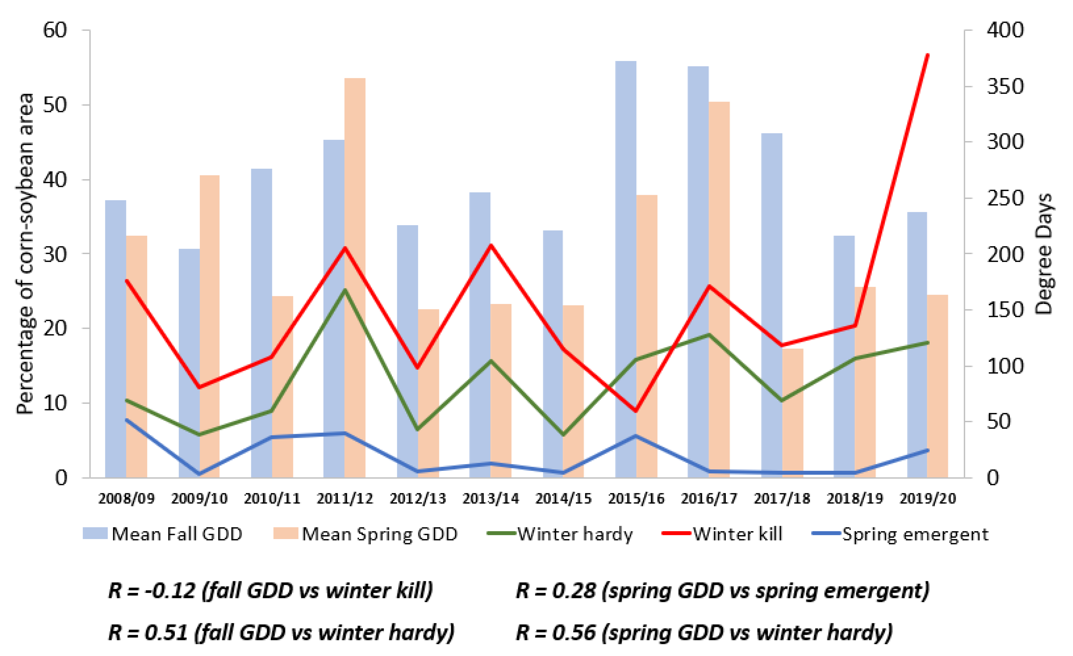
2.3. Weather Variability and Cover Crop Areas

To assess the potential influence of weather on cover crop growth, cumulative growing degree days (GDD) and total precipitation during the cover crop growing season were examined in relation to the geographic extent of estimated annual four cover crop classes. Cumulative GDD were calculated using daily average temperatures (Tmean) over the two cover crop growing seasons—fall (1 October through 31 December) and spring (1 January through 31 April) (with a base temperature (Tbase) of 5 °C annually) (Equation (3)). Similarly, total precipitatison for the months of October and November, the months when cover crops are usually planted in the Midwest, were considered. This was done in GEE using the PRISM Daily Spatial Climate Dataset with a spatial resolution of 2.5 arc minutes (~4 km) [39].
GDD = Tmean Tbase   if   Tmean > Tbase GDD = 0   if   Tmean < Tbase
where Tmean = (Tmin + Tmax)/2; Tbase = base temperature, Tmin = minimum temperature, and Tmax = maximum temperature.

3. Results

3.1. Accuracy Assessment

The classification of cover crops resulted in an overall accuracy (OA) of 74.7% and Kappa coefficient of 0.63 (Table 4). Of the four classes, the Not Covered class had the highest PA and UA, followed by the Winter Kill class. The Spring Emergent class had the lowest PA and UA of 57.4% and 40.1%, respectively. This shows that 57% of the ground-truth pixels in the Spring Emergent class were correctly classified, while only 40% of the total predicted pixels in the Spring Emergent class actually represented the true class. About 40% and 21% of the total predicted pixels in the Spring Emergent class were from the Winter Hardy and Not Covered classes, respectively. This suggests a subtle within field variability in pixel values representing Spring Emergent and Winter Hardy cover crop classes.

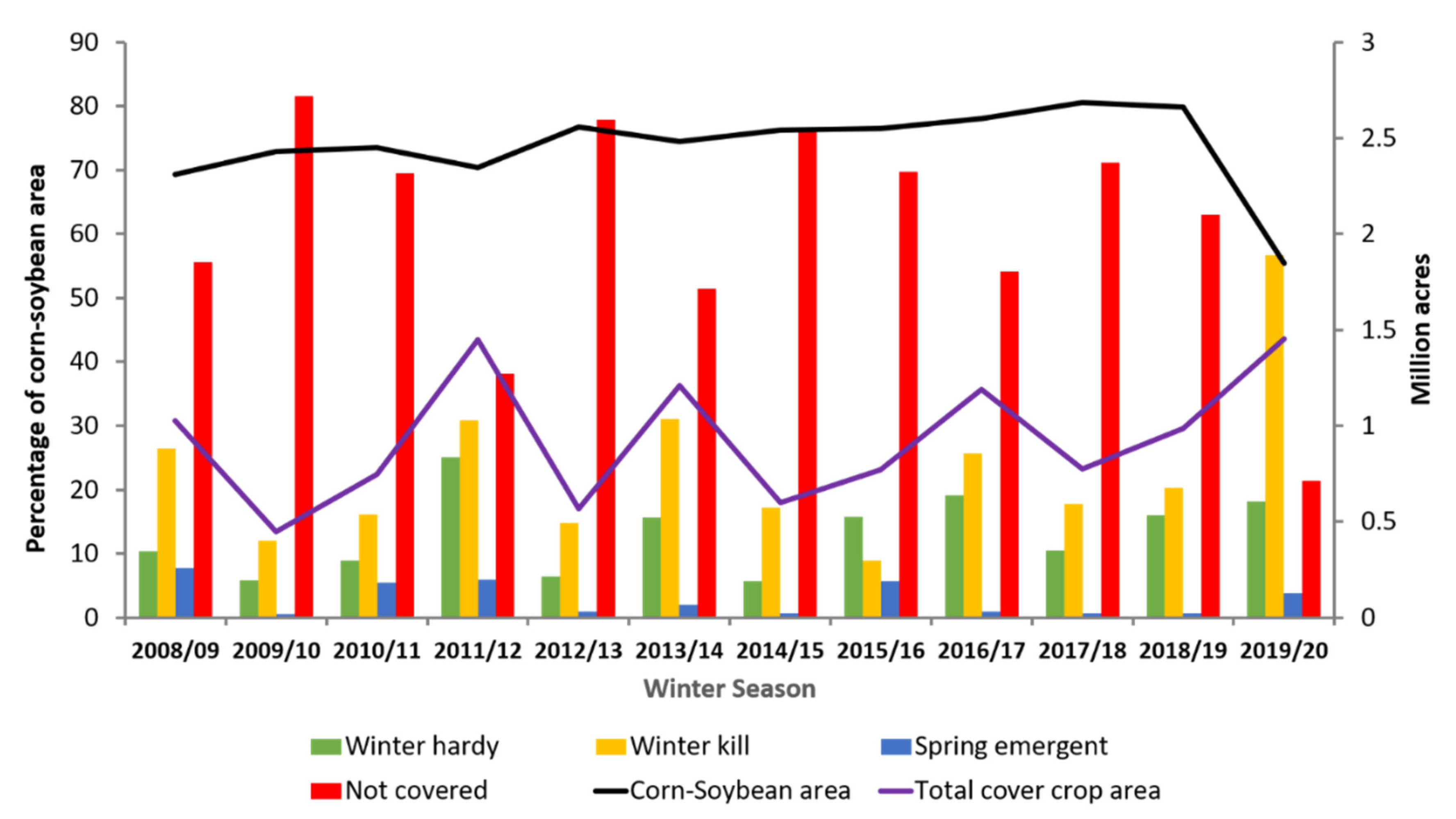
3.2. Cover Crop Areas: Temporal Patterns

Cover crop maps for the period of 2008/2009 to 2019/2020 suggested that about 11% to 34% of MRW areas were planted in cover crops (including Winter Hardy, Winter Kill, and Spring Emergent), with 2011/2012 and 2019/2020 having the largest cover crop areas and 2009/2010 the least (Figure 5). When cover crop areas were compared with total corn and soybean areas annually, there was a negative correlation (−0.52) between them. Except for 2019 (very wet summer, discussed in the Discussion section), the total corn-soybean areas remained relatively stable (i.e., 54–62%) throughout the study period. In general, less than 50% of corn-soybean fields were estimated to incorporate cover crops (Figure 6).
Although the total cover crop area increased between 2008/2009 and 2010/2011, there lacked a consistent increase in annual cover crop areas between 2008/2009 and 2019/2020 in general. Additionally, only 0.3% of the total watershed areas was consistently planted in cover crops for 12 years, with 20% of areas for more than five years and more than 50% areas for less than five years.

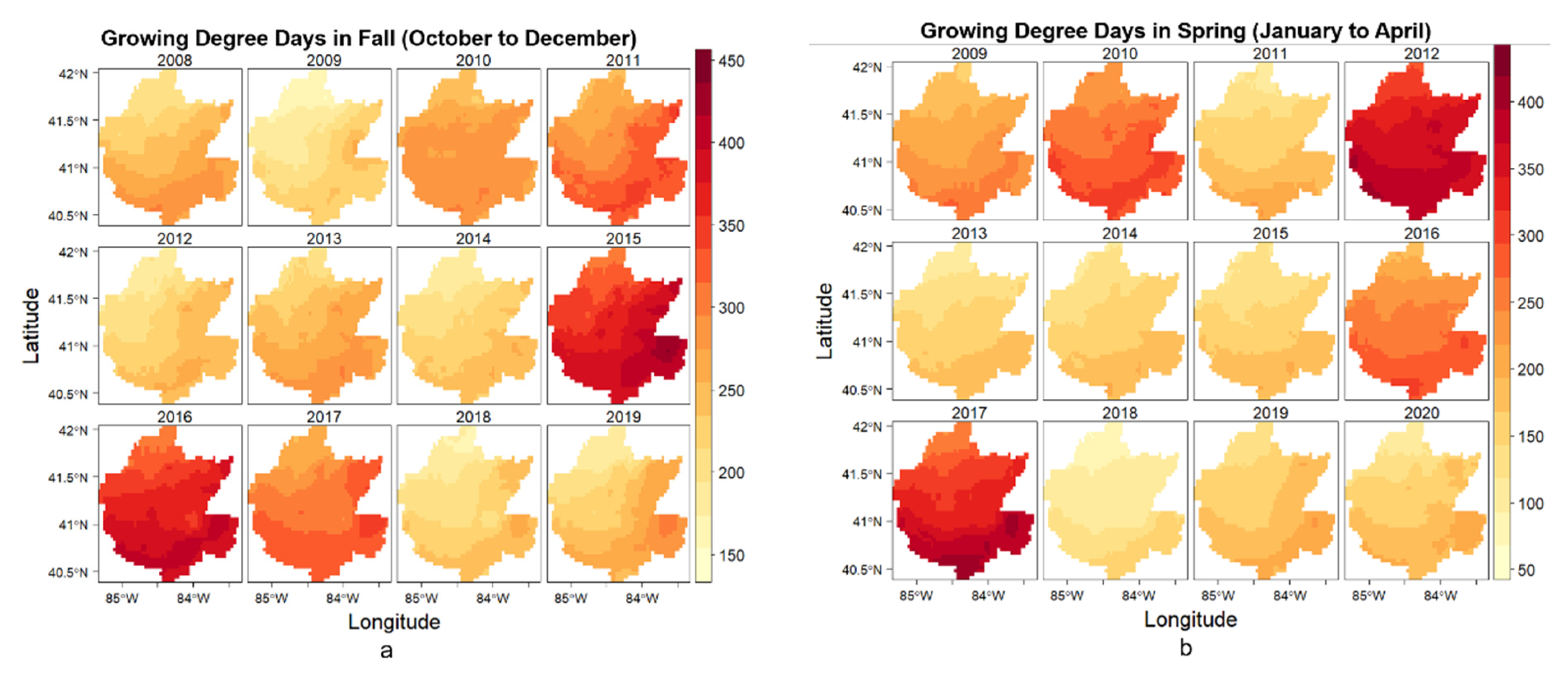
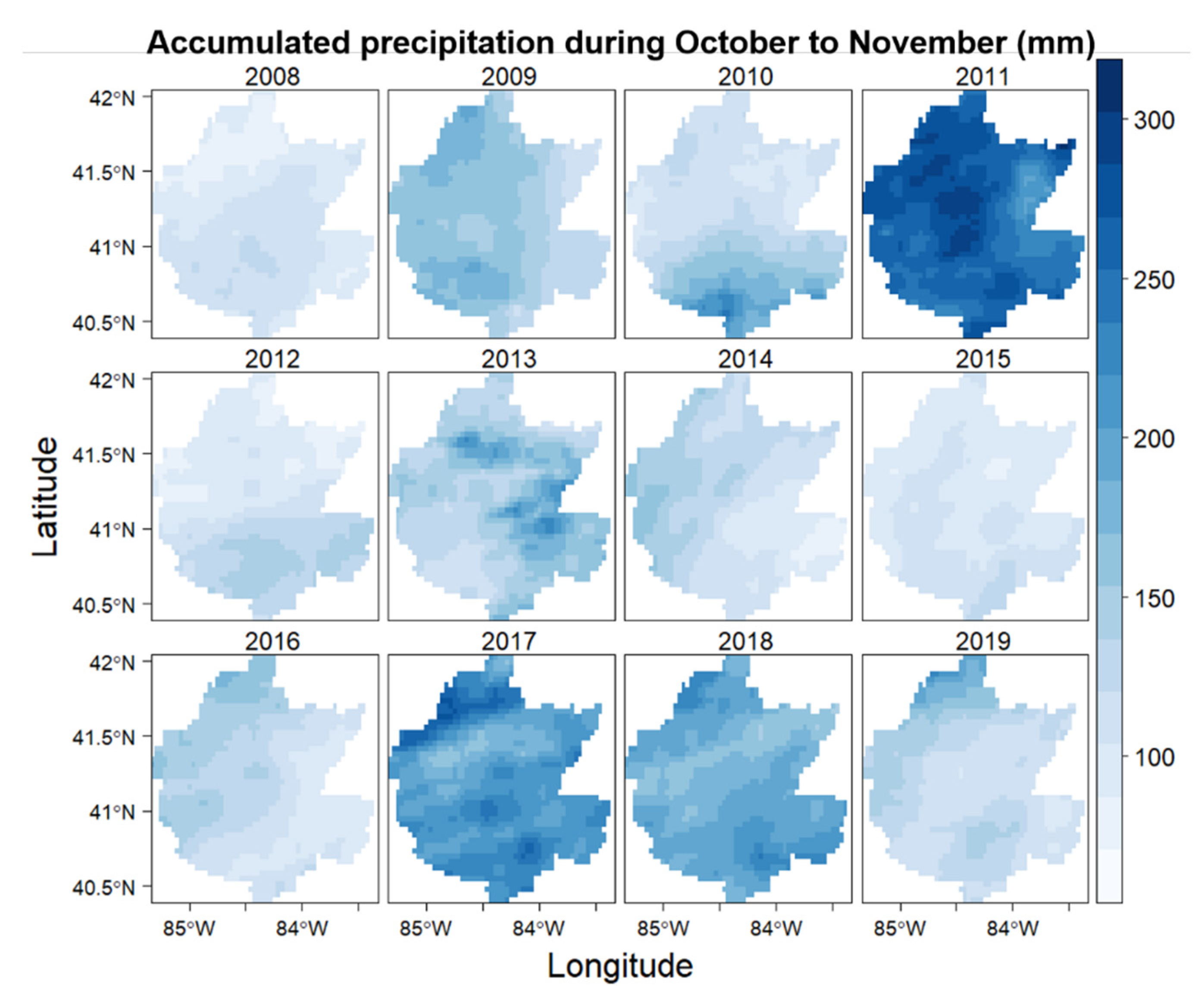
3.3. Effects of Weather on Variation in Winter Cover

When cover crop areas were evaluated in relation to GDD for fall and spring, higher GDDs were found to have a positive influence on cover crop performance (Figure 7). Specifically, years with a higher Winter Hardy cover crop area overlapped with years that had a higher GDD for fall (R = 0.51) and spring (R = 0.56). Although spring GDD was found to be positively correlated with Spring Emergent cover crop areas (R = 0.28), this correlation was not as strong as the correlation between fall GDD and Winter Hardy cover crop areas. Fall GDDs however were found to be less correlated (R = −0.11) with Winter Kill cover crops. In 2019, Winter Kill cover crop areas increased dramatically and showed no relation with GDD (R = 0.05).
Similar to GDDs, total fall precipitation was found to have a positive impact on cover crop areas, suggesting that a higher cumulative GDD and fall precipitation help promote cover crop establishment as well as their growth throughout the season. For instance, cover crop areas were higher in years of 2011/2012, 2016/2017 and 2017/2018 that also had higher fall precipitation and cumulative GDDs (Figure 8 and Figure 9).

4. Discussions

4.1. Training Dataset

In this study, we developed a detailed GEE framework to classify cover crop areas by integrating publicly available Landsat satellite images with ground-truth observations and tested it for the MRW. Satellite images were collected during cover crop growing season from October until April. Using the pixel reducer function in GEE, the satellite images were converted into two median seasonal composites: first composite (October to December) and second composite (January to April). In addition to median pixels values of individual bands and indices, maximum and minimum composites of NDVI were added to improve the classification between cover cropped and non cover cropped fields. Ground truth data on location of cover cropped fields were used to extract the pixel values from the composites and develop training and validation dataset. A RF model was trained with the training data, which was then applied on each seasonal composite in GEE to classify into four types of cover: Winter Hardy, Winter Kill, Spring Emergent, and No Cover. The overall classification accuracy of the model was 75% based on the independent validation dataset, with classes such as Winter Hardy and Not Covered crop classified with higher accuracy ranging between 75–80% and spring emergent classified with lower accuracy (57%). These classification accuracies can be attributed to the size and nature of the available ground-truth data.
In the study, a database of ground-truth cover crop fields was prepared through digitization of tillage transect survey data that were collected once during spring per year (discussed in the method section). There were some fields which surveys indicated to have cover crops, but satellite imagery consistently showed poor vegetation. Since vegetation health varies with field conditions and/or management practices and ground-truth data were collected at a single point of time, we relied on NDVI to assess seasonal growth of cover crops, as well as to group ground-truth cover crop fields into various classes. We think, however, that ground-truth cover crop growth information from multiple time points, if available, would help improve the accuracy of cover crop classification model.
In the study, misclassification was prominent for the Spring Emergent class, which can be attributed to a fewer dataset available for training and testing of the RF classifier for this class. It is expected that cover crops with no emergence, or slow growth in the fall, would have poor growth in the spring; thus, this results in a lower probability for fields to be in that category. This could be the reason that only 24 fields out of total 628 were grouped as Spring Emergent; a relatively small dataset to train and test the RF classifier for a large landscape as considered in this study. Although there is no set standard for training and testing data size suitable to address this sort of classification problem, an increase in ground-truth data usually increases classification accuracy.

4.2. Pixel Based Classification and Preparation of Training Dataset

The approach used to group the ground-truth fields into four cover crop classes could be another source of classification error. These fields were grouped based on their average greenness, i.e., NDVI estimated based on Landsat images collected during fall and spring seasons (Figure 3). In this process, any fields with an average NDVI value below 0.3 were classified as Not Covered. However, there could have been areas within the field for which NDVI values were either higher or lower than the average. Since all the pixels within a field were labeled the same and are used for training the RF algorithm, this could lead to misclassification in a field and/or area with high with-in field variability in cover crop growth. This could be one of the reasons why a large proportion of Spring Emergent pixels were misclassified as Not Covered and Winter Hardy classes, and some areas in a landscape appeared to have a salt and pepper alike distribution of cover crop classes (Figure 5). Although the approach used in our study is widely practiced [15,20,36,38], this problem may be resolved by dividing a field into multiple zones and training the classification model accordingly.
Salt and pepper-like distribution of cover crop classes are typical of the pixel-based classification approach where the spectral signature of a pixel is evaluated independently of its surrounding pixels. In addition to natural microvariability within a field (e.g., soil, topography), artificial factors (e.g., SLC off in case of Landsat 7; compositing and fusion of images from multiple satellite sensors) can have a big impact on spectral properties of pixels, and thus the overall training and testing of the classification model. For instance, compositing helps to fill in the data gap, but it can introduce some forms of artifacts when images have a high amount of scan line errors, one of the problems that is difficult to address when it comes to application of satellite images.

4.3. Variation in Winter Cover and Effects of Weather

When the impact of weather, mainly precipitation and GDD, was evaluated on spatial and temporal variability in cover crop distribution in the MRW, we found fall precipitation to have a higher correlation with cover crop areas, which is in agreement with prior studies [40,66]. Fall precipitation is important to cover crop emergence, mainly to those that are aerially seeded, as increased soil moisture after rainfall helps increase the soil to seed contact required for germination. In a two-year field study, Gaudlip et al. [66] observed differences in cover crop emergence and stand establishment through aerial seeding and related those differences with fall precipitation [66]. Particularly, they observed lower emergence and stand establishment with low fall precipitation in 2017 and higher success in cover crop establishment in the very wet fall of 2018 when seeds were aerially applied. However, they found very wet condition unfavorable for cover crop emergence when seeds were drilled. The study also found fall biomass of cover crops to be correlated well with GDD for both years (R2 = 0.28 in 2017 and 0.82 in 2018) [66]. While it is difficult to differentiate cover crop by planting methods via remote sensing, it is important to understand the role of field topography and weather on cover crop emergence under various planting methods.
In this study, weather was found to be one of the factors influencing the adoption of cover crops. We observed increase in cover crop areas particularly in years with higher fall GDD (R = 0.13) and precipitation (R = 0.22). For instance, 2019/2020 is a good example of an abnormal wet year (January to August was the wettest period in 125 years) [67], which delayed planting of cash crops by about three to four weeks in the midwest, including Ohio. Specifically, in Ohio, during the second week of May, only 1–4% of the total corn and soybean acres were planted compared to 47% area for corn and 20% area for soybean for 2014–2018 (50% corn and 28% soybean in 2019 alone) [68]. The Ohio NRCS announced disaster recovery funding to farmers to plant cover crops on their flooded cropland instead of the regular cash crops [69]. This resulted in many farmers adopting cover crops in their corn/soybean fields [69], which was also evident in the 2019/2020 cover crop map (Figure 5) that showed more than 50% of corn/soybean areas in cover crops. In general, cover crop area increased by about 37% in MRW from 2012 to 2017, which is in agreement with the 2017 Census of Agriculture [70] that reported 50% increase in cover crop areas nationally.

4.4. Weed versus Cover Crops

Our cover crop classification model treats weeds and cover crops similarly if they have spectrally similar patterns. There is also a higher probability of corn/soybean fields being infested with weeds during fall when GDDs are higher than the normal [40]. These could be the reasons we observed a larger proportion of areas in Winter Kill and Winter Hardy cover crops in years with higher Fall GDDs. This argument is supported by prior studies based on field experiments. Baraibar et al. [40] reported that there exists a positive correlation between cover crop and weed biomass in the fall. However, this relationship is opposite during spring, as weeds are suppressed with increase in cover crop biomass. In summary, since the cover crop classification model developed in this study does not have an ability to differentiate between weeds and cover crops, caution needs to be paid while interpreting some of these results. If the goal of the classification is to separate weeds from cover crops, there will be a need for ground-truth data on cover crop and weed fields.

5. Conclusions

The study used a RF classifier on the Landsat satellite data in the GEE platform to quantify spatial and temporal trends of winter cover crops in the MRW in northwestern Ohio between 2008–2019. The estimated cover crop areas were examined in relation to GDD and temperature to understand the effect of temperature and precipitation on cover crop growth. At first, satellite images were converted to seasonal composites in GEE, which were then used with ground-truth data to develop training and validation datasets. To develop the RF model, satellite derived covariates were trained using the training dataset and used to classify the satellite images into four different types of winter covers. The classified cover crop maps suggested an average of 39% of corn/soybean areas covered with cover crops for the period of 2008/2009 to 2019/2020. The classified cover crop map of 2019/2020 clearly captured an abnormally wet year when disaster recovery funding was available to most of the corn/soybean farmers to plant their fields with cover crops during fall. Winter cover crop areas in the MRW increased to about 78% in 2019/2020 season compared to the 2018/2019 season when cover crop areas were 37% of total corn/soybean areas. Cover crops were found to perform well when both GDDs and fall precipitation were favorable during early establishment as well as through the entire winter season. This study showed that the cover cropping practice can be monitored at a landscape scale by utilizing publicly available images from satellites. Understanding the spatial and temporal trends of cover crops at a landscape scale, as estimated in this study, is useful in promoting site-specific cover crop management practices to enhance their environmental benefits. This is also valuable to policy makers as well as funding agencies to localize areas in need of interventions for supporting adoption of cover cropping practice for improving an overall sustainability of agricultural production system.

Author Contributions

Conceptualization, S.K. and K.K.; methodology, K.K.; software, K.K.; validation, K.K., S.K. and K.Z.; formal analysis, K.K.; investigation, K.K.; resources, S.K.; data curation, K.K.; writing—original draft preparation, K.K.; writing—review and editing, S.K.; Data collection and editing, M.R.; visualization, K.K.; supervision, S.K.; project administration, S.K.; funding acquisition, S.K. and K.Z. All authors have read and agreed to the published version of the manuscript.

Funding

This work was supported by funds from OSU L&L Grant# PG107271, SI Grant # PG107338, ODHE Grant #GR119061, and Hatch Project #NC1195.

Acknowledgments

Thanks are extended to Brigitte Moneymaker, Boden Fisher, and Jordan Beck—OSU water quality associates, and Soil Water and Conservation Districts of Crawford, Sandusky, Wyandot, Erie, Huron, and Fulton counties for their help in ground-truth data collection. We also acknowledge Breann Hohman from Erie Conservation district and Kevin King’s group at USDA ARS for providing additional data.

Conflicts of Interest

The authors declare no conflict of interest. The funders had no role in the design of the study; in the collection, analyses, or interpretation of data, in the writing of the manuscript or in the decision to publish the results.

References

  1. Dabney, S.M.; Delgado, J.A.; Reeves, D.W. Using winter cover crops to improve soil and water quality. Commun. Soil Sci. Plant Anal. 2001, 32, 1221–1250. [Google Scholar] [CrossRef]
  2. Sharpley, A.N.; Daniel, T.; Gibson, G.; Bundy, L.; Cabrera, M.; Sims, T.; Stevens, R.; Lemunyon, J.; Kleinman, P.; Parry, R. Best Management Practices to Minimize Agricultural Phosphorus Impacts on Water Quality; ARS-163; USDA-ARS: Washington, DC, USA, 2006.
  3. Villamil, M.B.; Bollero, G.A.; Darmody, R.G.; Simmons, F.W.; Bullock, D.G. No-Till Corn/Soybean Systems Including Winter Cover Crops. Soil Sci. Soc. Am. J. 2006, 70, 1936–1944. [Google Scholar] [CrossRef]
  4. Strock, J.S.; Porter, P.M.; Russelle, M.P. Cover Cropping to Reduce Nitrate Loss through Subsurface Drainage in the Northern U.S. Corn Belt. J. Environ. Qual. 2004, 33, 1010–1016. [Google Scholar] [CrossRef]
  5. Muenich, R.L.; Kalcic, M.; Scavia, D. Evaluating the Impact of Legacy P and Agricultural Conservation Practices on Nutrient Loads from the Maumee River Watershed. Environ. Sci. Technol. 2016, 50, 8146–8154. [Google Scholar] [CrossRef] [PubMed]
  6. Parr, M.; Grossman, J.M.; Reberg-Horton, S.C.; Brinton, C.; Crozier, C. Nitrogen Delivery from Legume Cover Crops in No-Till Organic Corn Production. Agron. J. 2011, 103, 1578–1590. [Google Scholar] [CrossRef]
  7. Behnke, G.D.; Villamil, M.B. Cover crop rotations affect greenhouse gas emissions and crop production in Illinois, USA. Field Crop. Res. 2019, 241, 107580. [Google Scholar] [CrossRef]
  8. Brennan, E.B.; Smith, R.F. Winter Cover Crop Growth and Weed Suppression on the Central Coast of California. Weed Technol. 2005, 19, 1017–1024. [Google Scholar] [CrossRef]
  9. Wilcoxen, C.A.; Walk, J.W.; Ward, M.P. Use of cover crop fields by migratory and resident birds. Agric. Ecosyst. Environ. 2018, 252, 42–50. [Google Scholar] [CrossRef]
  10. Rundquist, S.; Carlson, S. Mapping Cover Crops on Corn and Soybeans in Illinois, Indiana and Iowa, 2015–2016; Environmental Working Group: Washington, DC, USA, 2017. [Google Scholar]
  11. Roesch-Mcnally, G.E.; Basche, A.D.; Arbuckle, J.G.; Tyndall, J.C.; Miguez, F.E.; Bowman, T.; Clay, R. The trouble with cover crops: Farmers’ experiences with overcoming barriers to adoption. Renew. Agric. Food Syst. 2018, 33, 322–333. [Google Scholar] [CrossRef] [Green Version]
  12. CTIC. Annual Report 2019–2020 National Cover Crop Survey; CTIC: West Lafayette, IN, USA, 2020. [Google Scholar]
  13. Hagen, S.C.; Delgado, G.; Ingraham, P.; Cooke, I.; Emery, R.; Fisk, J.P.; Melendy, L.; Olson, T.; Patti, S.; Rubin, N.; et al. Mapping conservation management practices and outcomes in the corn belt using the operational tillage information system (Optis) and the denitrification–decomposition (DNDC) model. Land 2020, 9, 408. [Google Scholar] [CrossRef]
  14. Tao, Y.; You, F. Prediction of Cover Crop Adoption through Machine Learning Models using Satellite-derived Data. IFAC Pap. 2019, 52, 137–142. [Google Scholar] [CrossRef]
  15. Seifert, C.A.; Azzari, G.; Lobell, D.B. Satellite detection of cover crops and their effects on crop yield in the Midwestern United States. Environ. Res. Lett. 2018, 14. [Google Scholar] [CrossRef]
  16. Thieme, A.; Yadav, S.; Oddo, P.C.; Fitz, J.M.; McCartney, S.; King, L.A.; Keppler, J.; McCarty, G.W.; Hively, W.D. Using NASA Earth observations and Google Earth Engine to map winter cover crop conservation performance in the Chesapeake Bay watershed. Remote Sens. Environ. 2020, 248, 111943. [Google Scholar] [CrossRef]
  17. Hively, W.D.; Duiker, S.; McCarty, G.; Prabhakara, K. Remote sensing to monitor cover crop adoption in southeastern Pennsylvania. J. Soil Water Conserv. 2015, 70, 340–352. [Google Scholar] [CrossRef] [Green Version]
  18. USGS. Landsat 8 Collection 1 (C1) Land Surface Reflectance Code (LaSRC) Product Guide; USGS: Sioux Falls, SD, USA, 2020; Volume 1.
  19. Gorelick, N.; Hancher, M.; Dixon, M.; Ilyushchenko, S.; Thau, D.; Moore, R. Google Earth Engine: Planetary-scale geospatial analysis for everyone. Remote Sens. Environ. 2017, 202, 18–27. [Google Scholar] [CrossRef]
  20. Xiong, J.; Thenkabail, P.S.; Gumma, M.K.; Teluguntla, P.; Poehnelt, J.; Congalton, R.G.; Yadav, K.; Thau, D. Automated cropland mapping of continental Africa using Google Earth Engine cloud computing. ISPRS J. Photogramm. Remote Sens. 2017, 126, 225–244. [Google Scholar] [CrossRef] [Green Version]
  21. Xie, Y.; Lark, T.J.; Brown, J.F.; Gibbs, H.K. Mapping irrigated cropland extent across the conterminous United States at 30 m resolution using a semi-automatic training approach on Google Earth Engine. ISPRS J. Photogramm. Remote Sens. 2019, 155, 136–149. [Google Scholar] [CrossRef]
  22. Oliphant, A.J.; Thenkabail, P.S.; Teluguntla, P.; Xiong, J.; Gumma, M.K.; Congalton, R.G.; Yadav, K. Mapping cropland extent of Southeast and Northeast Asia using multi-year time-series Landsat 30-m data using a random forest classifier on the Google Earth Engine Cloud. Int. J. Appl. Earth Obs. Geoinf. 2019, 81, 110–124. [Google Scholar] [CrossRef]
  23. Campos-Taberner, M.; Moreno-Martínez, Á.; García-Haro, F.J.; Camps-Valls, G.; Robinson, N.P.; Kattge, J.; Running, S.W. Global Estimation of Biophysical Variables from Google Earth Engine Platform. Remote Sens. 2018, 10, 1167. [Google Scholar] [CrossRef] [Green Version]
  24. Traganos, D.; Aggarwal, B.; Poursanidis, D.; Topouzelis, K.; Chrysoulakis, N.; Reinartz, P. Towards Global-Scale Seagrass Mapping and Monitoring Using Sentinel-2 on Google Earth Engine: The Case Study of the Aegean and Ionian Seas. Remote Sens. 2018, 10, 1227. [Google Scholar] [CrossRef] [Green Version]
  25. Michalak, A.M.; Anderson, E.J.; Beletsky, D.; Boland, S.; Bosch, N.S.; Bridgeman, T.B.; Chaffin, J.D.; Cho, K.; Confesor, R.; Daloglu, I.; et al. Record-setting algal bloom in Lake Erie caused by agricultural and meteorological trends consistent with expected future conditions. Proc. Natl. Acad. Sci. USA 2013, 110, 6448–6452. [Google Scholar] [CrossRef] [PubMed] [Green Version]
  26. Kast, J.B.; Apostel, A.M.; Kalcic, M.M.; Muenich, R.L.; Dagnew, A.; Long, C.M.; Evenson, G.; Martin, J.F. Source contribution to phosphorus loads from the Maumee River watershed to Lake Erie. J. Environ. Manag. 2021, 279, 111803. [Google Scholar] [CrossRef]
  27. Martin, J.; Kalcic, M.; Aloysius, N.; Apostel, A.; Brooker, M.; Evenson, G.; Kast, J.; Kujawa, H.; Murumkar, A.; Becker, R.; et al. Evaluating management options to reduce Lake Erie algal blooms using an ensemble of watershed models. J. Environ. Manag. 2020, 280. [Google Scholar] [CrossRef]
  28. Ohio Department of Agriculture; Ohio Department of Natural Resources; Ohio Environmental Protection Agency; Ohio Lake Erie Commission. Ohio Lake Erie Phosphorus Task Force Final Report; Ohio Environmental Protection Agency: Columbus, OH, USA, 2013.
  29. Stumpf, R.P.; Wynne, T.T.; Baker, D.B.; Fahnenstiel, G.L. Interannual Variability of Cyanobacterial Blooms in Lake Erie. PLoS ONE 2012, 7, e42444. [Google Scholar] [CrossRef] [PubMed]
  30. Foga, S.; Scaramuzza, P.L.; Guo, S.; Zhu, Z.; Dilley, R.D.; Beckmann, T.; Schmidt, G.L.; Dwyer, J.L.; Joseph Hughes, M.; Laue, B. Cloud detection algorithm comparison and validation for operational Landsat data products. Remote Sens. Environ. 2017, 194, 379–390. [Google Scholar] [CrossRef] [Green Version]
  31. Vermote, E.; Justice, C.; Claverie, M.; Franch, B. Preliminary analysis of the performance of the Landsat 8/OLI land surface reflectance product. Remote Sens. Environ. 2016, 185, 46–56. [Google Scholar] [CrossRef]
  32. Masek, J.G.; Vermote, E.F.; Saleous, N.E.; Wolfe, R.; Hall, F.G.; Huemmrich, K.F.; Gao, F.; Kutler, J.; Lim, T.-K. A Landsat surface reflectance dataset for North America, 1990–2000. IEEE Geosci. Remote Sens. Lett. 2006, 3, 68–72. [Google Scholar] [CrossRef]
  33. Roy, D.P.; Kovalskyy, V.; Zhang, H.K.; Vermote, E.F.; Yan, L.; Kumar, S.S.; Egorov, A. Characterization of Landsat-7 to Landsat-8 reflective wavelength and normalized difference vegetation index continuity. Remote Sens. Environ. 2016, 185, 57–70. [Google Scholar] [CrossRef] [Green Version]
  34. Vogeler, J.C.; Braaten, J.D.; Slesak, R.A.; Falkowski, M.J. Extracting the full value of the Landsat archive: Inter-sensor harmonization for the mapping of Minnesota forest canopy cover (1973–2015). Remote Sens. Environ. 2018, 209, 363–374. [Google Scholar] [CrossRef]
  35. Savage, S.L.; Lawrence, R.L.; Squires, J.R.; Holbrook, J.D.; Olson, L.E.; Braaten, J.D.; Cohen, W.B. Shifts in Forest Structure in Northwest Montana from 1972 to 2015 Using the Landsat Archive from Multispectral Scanner to Operational Land Imager. Forests 2018, 9, 157. [Google Scholar] [CrossRef] [Green Version]
  36. Azzari, G.; Grassini, P.; Edreira, J.I.R.; Conley, S.; Mourtzinis, S.; Lobell, D.B. Satellite mapping of tillage practices in the North Central US region from 2005 to 2016. Remote Sens. Environ. 2019, 221, 417–429. [Google Scholar] [CrossRef]
  37. Carrasco, L.; O’Neil, A.W.; Morton, R.D.; Rowland, C.S. Evaluating Combinations of Temporally Aggregated Sentinel-1, Sentinel-2 and Landsat 8 for Land Cover Mapping with Google Earth Engine. Remote Sens. 2019, 11, 288. [Google Scholar] [CrossRef] [Green Version]
  38. Teluguntla, P.; Thenkabail, P.; Oliphant, A.; Xiong, J.; Gumma, M.K.; Congalton, R.G.; Yadav, K.; Huete, A. A 30-m landsat-derived cropland extent product of Australia and China using random forest machine learning algorithm on Google Earth Engine cloud computing platform. ISPRS J. Photogramm. Remote Sens. 2018, 144, 325–340. [Google Scholar] [CrossRef]
  39. Oregon State University PRISM Climate Group. Available online: https://prism.oregonstate.edu (accessed on 11 May 2020).
  40. Baraibar, B.; Mortensen, D.A.; Hunter, M.C.; Barbercheck, M.E.; Kaye, J.P.; Finney, D.M.; Curran, W.S.; Bunchek, J.; White, C.M. Growing degree days and cover crop type explain weed biomass in winter cover crops. Agron. Sustain. Dev. 2018, 38, 65. [Google Scholar] [CrossRef] [Green Version]
  41. Ghazaryan, G.; Dubovyk, O.; Löw, F.; Lavreniuk, M.; Kolotii, A.; Schellberg, J.; Kussul, N. A rule-based approach for crop identification using multi-temporal and multi-sensor phenological metrics. Eur. J. Remote Sens. 2018, 51, 511–524. [Google Scholar] [CrossRef]
  42. Davis, J.; Sampson, R. Statistics and Data Analysis in Geology; Wiley: New York, NY, USA, 1986. [Google Scholar]
  43. Jakubauskas, M.E.; Legates, D.R.; Kastens, J.H. Harmonic analysis of time-series AVHRR NDVI data. Photogramm. Eng. Remote Sens. 2001, 67, 461–470. [Google Scholar]
  44. Jakubauskas, M.E.; Legates, D.R.; Kastens, J.H. Crop identification using harmonic analysis of time-series AVHRR NDVI data. Comput. Electron. Agric. 2002, 37, 127–139. [Google Scholar] [CrossRef]
  45. USDA CropScape-Cropland Data Layer. Available online: https://nassgeodata.gmu.edu/CropScape/ (accessed on 1 May 2020).
  46. Townshend, J.R.G.; Justice, C.O. Analysis of the dynamics of African vegetation using the normalized difference vegetation index. Int. J. Remote Sens. 1986, 7, 1435–1445. [Google Scholar] [CrossRef]
  47. Wardlow, B.D.; Egbert, S.L. Large-area crop mapping using time-series MODIS 250 m NDVI data: An assessment for the U.S. Central Great Plains. Remote Sens. Environ. 2008, 112, 1096–1116. [Google Scholar] [CrossRef]
  48. Bellón, B.; Bégué, A.; Lo Seen, D.; De Almeida, C.A.; Simões, M. A Remote Sensing Approach for Regional-Scale Mapping of Agricultural Land-Use Systems Based on NDVI Time Series. Remote Sens. 2017, 9, 600. [Google Scholar] [CrossRef] [Green Version]
  49. Tucker, C.J. Red and photographic infrared linear combinations for monitoring vegetation. Remote Sens. Environ. 1979, 8, 127–150. [Google Scholar] [CrossRef] [Green Version]
  50. Jordan, C.F. Derivation of Leaf-Area Index from Quality of Light on the Forest Floor. Ecology 1969, 50, 663–666. [Google Scholar] [CrossRef]
  51. Tian, H.; Huang, N.; Niu, Z.; Qin, Y.; Pei, J.; Wang, J. Mapping Winter Crops in China with Multi-Source Satellite Imagery and Phenology-Based Algorithm. Remote Sens. 2019, 11, 820. [Google Scholar] [CrossRef] [Green Version]
  52. Moreno-Martínez, Á.; Izquierdo-Verdiguier, E.; Maneta, M.P.; Camps-Valls, G.; Robinson, N.; Muñoz-Marí, J.; Sedano, F.; Clinton, N.; Running, S.W. Multispectral high resolution sensor fusion for smoothing and gap-filling in the cloud. Remote Sens. Environ. 2020, 247, 111901. [Google Scholar] [CrossRef]
  53. CTIC. Revised and Simplified Cropland Roadside Transect Survey; CTIC: West Lafayette, IN, USA, 2002. [Google Scholar]
  54. Haas, J.; Ban, Y. Urban growth and environmental impacts in Jing-Jin-Ji, the Yangtze, River Delta and the Pearl River Delta. Int. J. Appl. Earth Obs. Geoinf. 2014, 30, 42–55. [Google Scholar] [CrossRef]
  55. Belgiu, M.; Drǎguţ, L. Comparing supervised and unsupervised multiresolution segmentation approaches for extracting buildings from very high resolution imagery. ISPRS J. Photogramm. Remote Sens. 2014, 96, 67–75. [Google Scholar] [CrossRef] [Green Version]
  56. Karlson, M.; Ostwald, M.; Reese, H.; Sanou, J.; Tankoano, B.; Mattsson, E. Mapping Tree Canopy Cover and Aboveground Biomass in Sudano-Sahelian Woodlands Using Landsat 8 and Random Forest. Remote Sens. 2015, 7, 10017–10041. [Google Scholar] [CrossRef] [Green Version]
  57. Frazier, R.J.; Coops, N.C.; Wulder, M.A.; Kennedy, R. Characterization of aboveground biomass in an unmanaged boreal forest using Landsat temporal segmentation metrics. ISPRS J. Photogramm. Remote Sens. 2014, 92, 137–146. [Google Scholar] [CrossRef]
  58. Nitze, I.; Schulthess, U.; Asche, H. Comparison of machine learning algorithms random forest, artificial neuronal network and support vector machine to maximum likelihood for supervised crop type classification. In Proceedings of the 4th GEOBIA, Rio de Janeiro, Brazil, 7–9 May 2012; pp. 35–40. [Google Scholar]
  59. Ok, A.O.; Akar, O.; Gungor, O. Evaluation of random forest method for agricultural crop classification. Eur. J. Remote Sens. 2012, 45, 421–432. [Google Scholar] [CrossRef]
  60. Rodriguez-Galiano, V.F.; Chica-Olmo, M.; Abarca-Hernandez, F.; Atkinson, P.M.; Jeganathan, C. Random Forest classification of Mediterranean land cover using multi-seasonal imagery and multi-seasonal texture. Remote Sens. Environ. 2012, 121, 93–107. [Google Scholar] [CrossRef]
  61. Breiman, L. Random Forests. Mach. Learn. 2001, 45, 5–32. [Google Scholar] [CrossRef] [Green Version]
  62. Pelletier, C.; Valero, S.; Inglada, J.; Champion, N.; Dedieu, G. Assessing the robustness of Random Forests to map land cover with high resolution satellite image time series over large areas. Remote Sens. Environ. 2016, 187, 156–168. [Google Scholar] [CrossRef]
  63. Belgiu, M.; Drăgu, L. Random forest in remote sensing: A review of applications and future directions. ISPRS J. Photogramm. Remote Sens. 2016, 114, 24–31. [Google Scholar] [CrossRef]
  64. Rodriguez-Galiano, V.F.; Ghimire, B.; Rogan, J.; Chica-Olmo, M.; Rigol-Sanchez, J.P. An assessment of the effectiveness of a random forest classifier for land-cover classification. ISPRS J. Photogramm. Remote Sens. 2012, 67, 93–104. [Google Scholar] [CrossRef]
  65. Gislason, P.O.; Benediktsson, J.A.; Sveinsson, J.R. Random forests for land cover classification. Pattern Recognit. Lett. 2006, 27, 294–300. [Google Scholar] [CrossRef]
  66. Gaudlip, C.; Sedghi, N.; Fox, R.; Sherman, L.; Weil, R. Effective Cover Cropping in Extremes of Weather; University of Maryland Extension: College Park, MD, USA, 2019; Volume 10. [Google Scholar]
  67. Yin, Y.; Byrne, B.; Liu, J.; Wennberg, P.O.; Davis, K.J.; Magney, T.; Köhler, P.; He, L.; Jeyaram, R.; Humphrey, V.; et al. Cropland Carbon Uptake Delayed and Reduced by 2019 Midwest Floods. AGU Adv. 2020, 1, 1–15. [Google Scholar] [CrossRef]
  68. USDA. Economics, Statistics and Market Information System. Available online: https://usda.library.cornell.edu/concern/publications/8336h188j?locale=en#release-items (accessed on 2 December 2020).
  69. USDA. NRCS Ohio NRCS Announces Disaster Recovery Funding to Plant Cover Crops on Flooded Cropland Acreage. Available online: https://www.nrcs.usda.gov/wps/portal/nrcs/oh/newsroom/releases/52bc20f8-c480-4908-848b-1546ca68a182/ (accessed on 5 February 2021).
  70. United States Department of Agriculture. 2017 Census of Agriculture; United States Department of Agriculture: Washington, DC, USA, 2019; Volume 1.
Figure 1. Maumee River watershed spreading over Ohio, Indiana and Michigan in the Midwest United States.
Remotesensing 13 02689 g001
Figure 2. Historical minimum, maximum and mean temperature for the MRW.
Remotesensing 13 02689 g002
Figure 3. Second order harmonic analyses of NDVI based on 255 fields from Erie and Huron counties in 2015/2016 (a), 2016/2017 (b), 2017/2018 (c) and 2018/2019 (d).
Remotesensing 13 02689 g003
Figure 4. Landsat satellite image composites before and after gap filling. Composite 1 represents fall growth (from October to December) and Composite 2 represents spring growth (from January to April).
Remotesensing 13 02689 g004
Figure 5. (Top) Cover crop maps for the Maumee River Watershed between 2008/2009 to 2019/2020, and (bottom) cover crop classes for 2019/2020 along with two seasonal composites and classification results for a small section of an area in the MRW to illustrate the process. Note: seasonal composites are shown using a natural color display of median of red, green, and blue bands.
Remotesensing 13 02689 g005
Figure 6. Annual variability of cover crop areas between 2008–2019. Note: the % area was computed based on total annual corn-soybean area per year. The x-axis represents the winter season. The total cover crop area represents all Winter Hardy, Winter Kill, and Spring Emergent classes. The secondary y-axis on the right represents areas (in terms of million acres) for either total cover crop or corn-soybean.
Remotesensing 13 02689 g006
Figure 7. Relationship between cover crops and GDD. Note: years in x-axis indicates fall of a prior year and spring of following year, left Y-axis indicates cover crop areas expressed in terms of % of corn/soybean areas, and right Y-axis indicates GDD.
Remotesensing 13 02689 g007
Figure 8. Fall (a) and spring (b) GDD calculated for the MRW using PRISM daily temperature data at 4 km spatial resolution. The years indicated in this figure correspond to the fall months of a given year.
Remotesensing 13 02689 g008
Figure 9. Total precipitation for the months of October and November.
Remotesensing 13 02689 g009
Table 1. Landsat satellite missions considered for the study.
DatasetData ProductsSpatial/Temporal ResolutionLaunch/Data Availability
Landsat 8 OLILevel-2 SR [31]30 m (16 days)2013 (2013–Present)
Landsat 7 ETM+Level-2 SR [32]1999 (2000–Present)
Landsat 5 TMLevel-2 SR [32]1984 (1984–2012)
Table 2. Bands and indices that are included in each seasonal composite. Each of these components are treated as features in cover crop classification model.
Composite BandDescriptionComposite BandDescription
Blue_medianMedian of blue bandDVI_medianMedian of DVI
Green_medianMedian of Green bandNDVI_medianMedian of NDVI
NIR_medianMedian of NIR bandNDVI_maxMaximum of NDVI
Red_medianMedian of Red bandNDVI_minMinimum of NDVI
SWIR1_medianMedian of SWIR1 bandNGRDI_medianMedian of NGRDI
SWIR2_medianMedian of SWIR2 bandRVI_medianMedian of RVI
NIR: Near Infrared, SWIR: Shortwave Infrared, DVI: Differences Vegetation Index, NDVI: Normalized Difference Vegetation Index, NGRDI: Normalized Green Red Difference Index, RVI: Ratio Vegetation Index.
Table 3. NDVI criteria to characterize winter cover crops growth.
CriteriaClassNumber of Fields
Fall NDVI and Spring NDVI ≥ 0.3Winter-Hardy338
Fall NDVI ≥ 0.3 and Spring NDVI < 0.3Winter Kill134
Fall NDVI < 0.3 and Spring NDVI ≥ 0.3Spring Emergent24
Fall NDVI and Spring NDVI < 0.3Not Covered132
Note: Fall NDVI: average NDVI during October to December. Spring NDVI: average NDVI during January to April. These NDVI values were estimated by averaging NDVI values for all the pixels that fall inside a field boundary. Field numbers by cover crop season: 131(2015/2016), 182(2016/2017), 83(2017/2018), 87(2018/2019), 145(2019/2020).
Table 4. Accuracy of classification results presented via confusion matrix.
Predicted
Ground-TruthClassWinter HardyWinter KillSpring
Emergent
Not CoveredTotalPA
Winter Hardy816889581395810,83475.39%
Winter Kill114443007987643866.79%
Spring Emergent27937843309146857.42%
Not Covered3021438441920311,38480.84%
Total98936670210411,45730,124
UA82.56%64.47%40.07%80.33%
Overall Accuracy = 74.7%Kappa = 0.63
Note: The rows indicate the actual number of pixels whereas columns represent the number of predicted pixels. The diagonal cells highlighted using bold represent the number of correctly classified pixels.
Publisher’s Note: MDPI stays neutral with regard to jurisdictional claims in published maps and institutional affiliations.

