Article

Direction-of-Arrival Estimation over Sea Surface from Radar Scattering Based on Convolutional Neural Network

1
State Key Laboratory of Remote Sensing Science, Aerospace Information Research Institute, Chinese Academy of Sciences, Beijing 100101, China
2
University of Chinese Academy of Sciences, Beijing 100049, China
3
College of Geomatics and Geoinformation, Guilin University of Technology, Guilin 541004, China
*
Author to whom correspondence should be addressed.
Remote Sens. 2021, 13(14), 2681; https://doi.org/10.3390/rs13142681
Submission received: 15 May 2021 / Revised: 23 June 2021 / Accepted: 5 July 2021 / Published: 7 July 2021

Abstract

:
Conventional direction-of-arrival (DOA) estimation methods are primarily used in point source scenarios and based on array signal processing. However, due to the local scattering caused by sea surface, signals observed from radar antenna cannot be regarded as a point source but rather as a spatially dispersed source. Besides, with the advantages of flexibility and comparably low cost, synthetic aperture radar (SAR) is the present and future trend of space-based systems. This paper proposes a novel DOA estimation approach for SAR systems using the simulated radar measurement of the sea surface at different operating frequencies and wind speeds. This article’s forward model is an advanced integral equation model (AIEM) to calculate the electromagnetic scattered from the sea surface. To solve the DOA estimation problem, we introduce a convolutional neural network (CNN) framework to estimate the transmitter’s incident angle and incident azimuth angle. Results demonstrate that the CNN can achieve a good performance in DOA estimation at a wide range of frequencies and sea wind speeds.

1. Introduction

Determining the direction of arrival (DOA) of the radar signal is a fundamental problem for sea surveillance. The task of DOA estimation is to identify the signal source directions in which the signal is transmitted. Conventional DOA estimation methods, including beamforming techniques [1,2,3] and subspace-based methods [4,5,6,7,8], are primarily used in point source scenarios. With the development of machine learning and artificial intelligence, neural network (NN) has been applied in the DOA estimation domain [9,10,11,12,13,14]. This method establishes training datasets with DOA labels first, and then derives a mapping from antenna outputs to signal directions with existing methods. The derived mapping is then used on test datasets to estimate signal directions. An NN-based DOA estimation is data driven and does not rely on pre-assumptions about array geometries and whether the antenna outputs are calibrated or not. They have been demonstrated to be computationally more efficient than subspace-based methods in simulations [14].
However, sea-surface-induced local scattering causes signals from a single source to arrive via different paths and at different angles. Therefore, the signals observed from radar antenna can then be regarded as a superposition of all contributions from different propagating paths. In this case, the source is no longer perceived as a point source but instead as a spatially dispersed source with mean DOA and spatial extent. Previous works have shown that the performance of point source DOA estimation methods is degraded [15,16,17]. Most approaches for DOA estimation of scattered sources utilize a model of the data covariance matrix, for example, maximum likelihood estimators [18,19,20,21,22]. The price to pay for this increased efficiency and accuracy is that those algorithms require a multidimensional search to find the estimates and converge to a local minimum. Another commonly used approach, the spatial smoothing algorithm [23,24], obtains the robustness at the expense of a reduced effective aperture.
Additionally, methods as mentioned above require many antenna elements to achieve a high degree of accuracy. As the number of antenna elements increases, the power consumption, size, and the cost of the system increase. In [25], artificial neural networks are used to decrease the size and weight and reduce the costs of components production and whole application systems in forming a beam from radiating complex microstrip antenna. Previous studies on DOA estimation of SAR system were realized by filtering the rough-surface induced clutter and then retrieving the clutter-surpassed target signals [26,27]. In this paper, we attempt to develop a new DOA estimation technique with low computational complexity and high estimation accuracy from a radar observation.
This paper proposes a two-dimensional DOA estimation method for a radar system under a special case where the incident signal is fully scattered from the sea surface. At this point, the received signal contains sea clutter. We utilize a convolutional neural network (CNN) to establish the relationship of radar measurements with their incident directions. The advanced integral equation model (AIEM) is applied as the forward model to simulate the sea surface electromagnetic scattering under different operating frequencies, observation geometry, and winds. The input of CNN are model-generated radar measurements added with speckle noise and the output is the related incidence location of the input scattering pattern.
The contributions of this article are briefed as follows:
We explore the DOA estimation problem under a special case where the incident signal is randomly scattered by sea surface. The effect of radar frequencies and wind speeds is taken into consideration as well.
We propose a CNN framework that makes use of underlying statistical characteristics of speckle noise-contaminated radar measurements to predict their related incidence location. By experiment, the CNN shows good performance in the DOA estimation problem, and the performance of CNN is not affected by the radar frequencies and wind speeds.
This paper is organized as follows: Section 2 gives the relevant background on the random rough surface scattering models, especially the AIEM model, and illustrates the sensitivity of the received signal to influential parameters. Section 3 formulates the DOA estimation by sea surface scattering measurement, and presents an algorithm to simulate the sea surface measurement dataset and basic notations used for illustration. Besides, we present the CNN structure and interpret how it fits our requirements in Section 3. In Section 4, implementation details and experimental results are presented. Section 5 discusses the DOA estimation results with state-of-the-art algorithms and limitations in the current work. Finally, the conclusions are summarized to close the paper.

2. Sea Surface Scattering Datasets Generated by AIEM

We first give the AIEM bistatic scattering model, followed by a sensitivity analysis of radar measurement to incidence location and receiver location under certain sea states.

2.1. Bistatic Scattering Model

Figure 1 depicts a geometry of bistatic radar scattering from the sea surface. Sea surface is assumed to be a randomly rough surface with known statistical properties; θ i and ϕ i are the incident angle and incident azimuth angle, respectively; θ s and ϕ s are the scattering angle and scattering azimuth angle of the receiver, respectively; ε 0 and μ 0 are the permittivity and permeability of the half free space; ε r and μ r are relative permittivity and of the sea; k ^ i is the incident wave vector and k ^ s is the scattered wave vector. k ^ i and k ^ s are defined as:
k x = k sin θ i cos ϕ i , k s x = k sin θ s cos ϕ s , k y = k sin θ i sin ϕ i , k s y = k sin θ s sin ϕ s , k z = k cos θ i , k s z = k cos θ s
For the purpose of this paper, we utilize the AIEM as a forward model to simulate the scattering process of the sea surface under different observation configurations and sea states. The AIEM model is an analytical model based on the integral equation method (IEM) [28,29,30]. Both the IEM and AIEM models have been used on sea surface microwave scattering and are in excellent agreement with radar measurements [31,32,33,34].
In original AIEM model [29], σ p q 0 can be written as:
σ p q 0 = k 2 2 exp [ σ 2 ( k i z 2 + k s z 2 ) ] × n = 1 σ 2 n n ! | I p q n | W ( n ) ( k s x k i x , k s y k i y )
where the polarization indices p and q represent the p -polarized ( v or h ) transmitted power and the q -polarized ( v or h ) received power; k is the wave number of incident wave in free space; k i x , k i y , k i z , k s x , k s y , and k s z are the coordinate projection of k ^ i and k ^ s ; σ is the root-mean-squared (RMS) height of rough surface; the explicit expression of I p q n is given in [30]; W ( n ) is the Fourier transform of the n -th power of the surface correlation function ρ s . For sea surface scattering, W ( n ) is relevant to the relative azimuth angle χ between the direction of sea wind ϕ w and ϕ i [35]:
W ( n ) ( k , χ ) = 0 2 π 0 ρ s n ( r , ϕ ) e j k r cos ( χ ϕ ) r d r d ϕ
An approximate representation of the sea surface correlation function is given by [36,37]:
ρ s ( r , ϕ ) = s 2 e r L t
where L t = L u cos 2 ϕ w + L c sin 2 ϕ w is the correlation length along ϕ w . L u is the correlation length in the upwind direction (along ϕ w = 0 ); L c is the correlation length in the crosswind direction (along ϕ w = 90 ). An approximate form for W ( n ) ( k , χ ) is given by [37]:
W ( n ) ( k , χ ) = ( s L t n ) 2 [ 1 + ( k L t n ) 2 ] 3 2
It has been successfully used in sea surface scattering computations.

2.2. Sensitivity of Received Signals to Incidence Location

Before devising an effective approach to DOA estimation, it is essential to conduct a sensitivity analysis of scattering responses to incidence location under specific surface parameters. According to Equations (1), (2), and (5), besides the incidence and observation location, the three rough surface parameters, including RMS height, correlation length, and dielectric constant, are related to bistatic scattering coefficients. For sea surface scattering, these parameters are influenced by sea wind speed and radar operating frequency. The values of L u , L c , and σ under different wind speeds and frequencies can be found in [37]. They are empirical values derived by fitting the rough surface scattering model with measured data. In what follows, we illustrate the bistatic hemispherical plots for the dependences of incidence location and wind direction and wind speed.
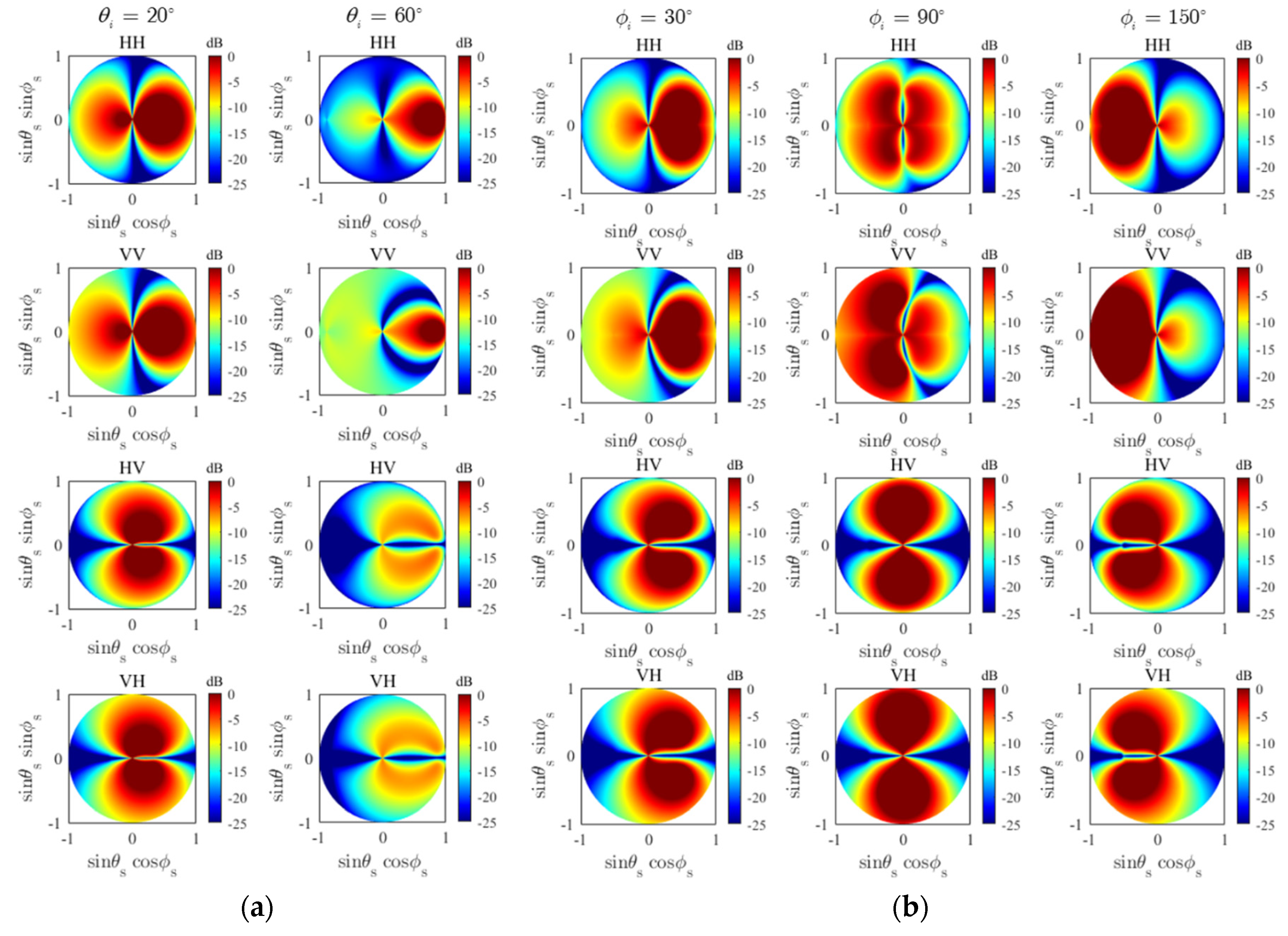
In Figure 2a,b, we examine the angular dependence of polarized bistatic scattering coefficients. Figure 2a shows the effect of the incident angle with f = 5.3 GHz, U = 25 m/s, ϕ i = 0 , θ i = 20 (the left column), and θ i = 60 (the right column). Similarly, Figure 2b shows the effect of the incident azimuth angle with f = 5.3 GHz, U = 25 m/s, θ i = 40 , ϕ i = 30 (the left column), ϕ i = 90 (the middle column), and ϕ i = 120 (the right column). For the same set of sea surface parameters, both the incident angle and incident azimuth angle have a strong influence on the scattering patterns and strength for all polarizations. In Figure 2a, the left-hand side of the half-sphere and right-hand side of the half-sphere represent backward and forward scattering regions. In contrast, the horizontal axis and vertical axis represent the incident plane and cross-incident plane. In the forward scattering region of Figure 2a, the strong scattering is due to the specular scattering, and it moves to the right hemisphere with the increase of the incident angle. For a smaller incident angle, the small azimuth angular region shows a stronger scattering strength at HH polarization. As the incident angle increases, the region with strong scattering starts to narrow down. In the backward region, the intensity of HH polarization reduces as the incident angle increases, but a subtle increment appears at a large scattering angle and scattering azimuth angle. Similar trends can be observed in VV polarization. Meanwhile, the strength of cross-polarization, HV and VH, quickly weakened on the whole upper hemisphere with an increasing incident angle. As for Figure 2b, the forward and backward scattering regions change with the incident azimuth angle. Relatively speaking, for all polarizations, the strong scattering area moves from the right-hand hemisphere to the left-hand hemisphere with the increase of the incident azimuth angle.
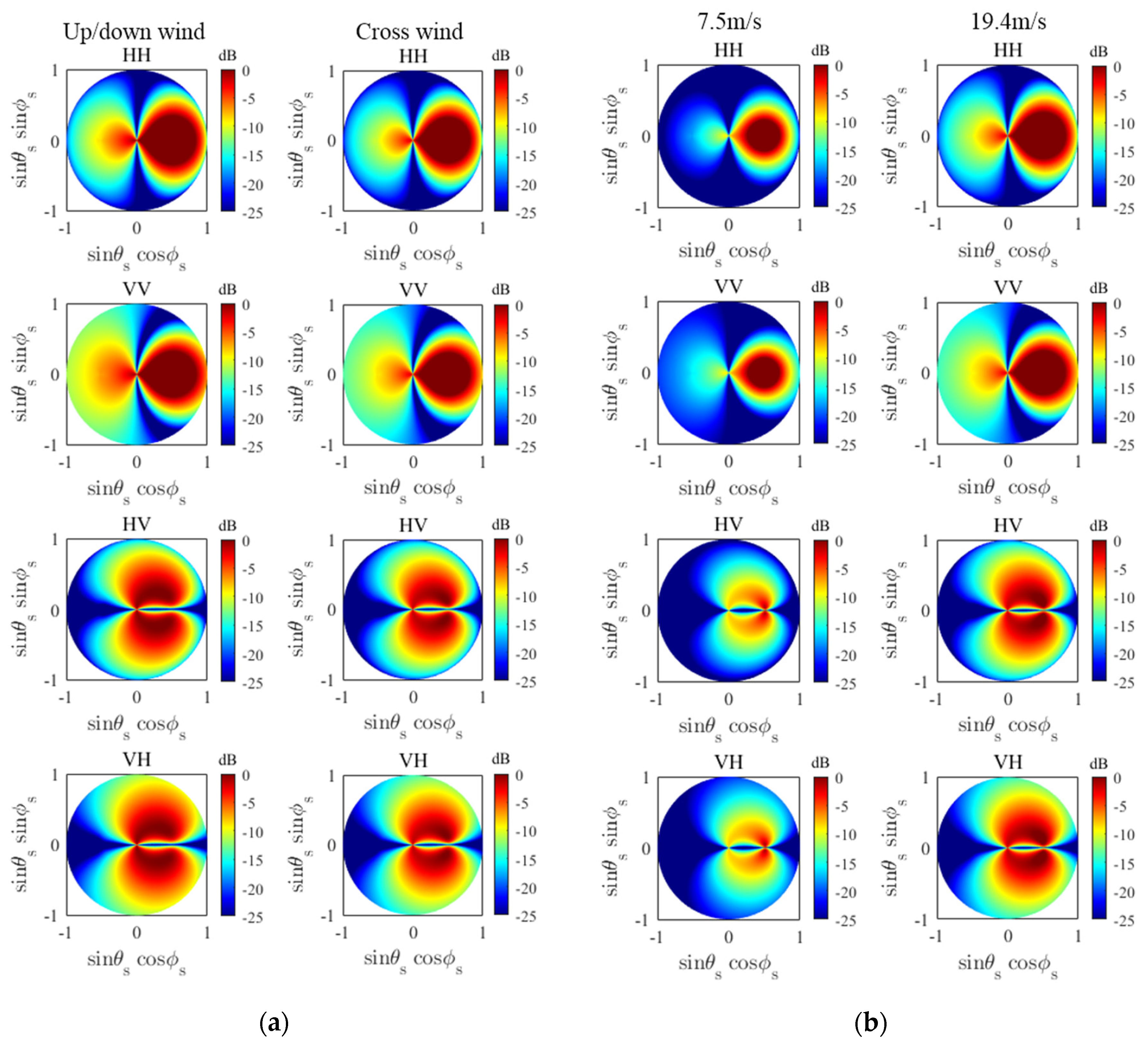
Figure 3a shows the hemispherical plot of co-and cross-polarized bistatic scattering coefficients with f = 5.3 GHz, U = 25 m/s, θ i = 30 , and ϕ i = 0 , with relative wind direction varying from up/downwind ( 0 / 180 ) to crosswind ( 90 ). For co-polarization, we see that the strong scattering area in the backward region at up/downwind is more pronounced than at crosswind. In addition, the cross-polarization is impacted by the relative wind direction to a lesser extent than co-polarization is.
Finally, we examine the sea surface roughness dependence in Figure 3b, which is the hemispherical plot of co-and cross-polarized bistatic scattering coefficients with f = 13.9 GHz, θ i = 30 , ϕ i = 0 , and ϕ w = 30 , but sea wind speed varying from 7.5 m/s to 19.4 m/s. With the increase of sea wind speeds, sea surface roughness is increased as well. However, the change of scattering coefficients is coupled with three roughness parameters. In general, the scattering strength under higher wind speed in both forward and backward regions is greater than the scattering strength under lower wind speed. Especially for cross-polarization under lower wind speed, there is a poorer feature in the backward scattering region than that in the forward region.

3. Direction-of-Arrival Estimation

3.1. Problem Formulation

To better estimate the angles of the incident source, a proper data model is essential to enable a mapping of the measurement domain to the feature domain that is of interest. We detail how we came up with a good scheme to improve DOA estimation accuracy and efficiency. The radar scattering from a rough surface can be modeled as [30]:
b = W x + u
where x is a vector including the surface parameters and radar parameters; matrix W relates the parameters vector x to radar scattering coefficients b ; and u represents the error vector induced by system and calibration errors, and speckle noise, among other factors. In this paper, the effect of speckle noise is considered only.
In statistical sense, x constitutes a random variable due to spatially and temporally varying properties, such that:
x = x t + x n
where x t is the true value and x n is the noise term. In practice, the “truth” is never obtainable and always vague. Statistically, x t and x n may be assumed to be uncorrelated, such that x is an unbiased estimation of x t , i.e.,
E ( x ) = E ( x t ) , x n N ( 0 , σ x n 2 )
where E denotes the statistical mean, and σ x n 2 is a variance of x n .
In general, the radar response is formed by the scattering matrix. For the purpose of this paper, we assume the radar measurement vector b is formed by multi-polarized scattering coefficients and the location of the scattering source:
b = [ σ h h 0 , σ v v 0 , σ h v 0 , σ v h 0 , θ s , ϕ s ] t
The location of the incident source is determined by the incident angle θ i and incident azimuth angle ϕ i . They are denoted by:
x = [ θ i , ϕ i ] t
Thus, the cost function of DOA estimation problem can be written as:
x ^ = arg min { | | b W x e s t | | 2 2 }
where | | · | | 2 denotes l 2 -norm and x e s t is the estimated incident angles.
Based on what we presented in last section, the scattering behavior is completely intricate. Therefore, it hard to get an analytical but practical solution of Equation (6). In this paper, we adapt a convolutional neural network approach for searching the cost function minima in Equation (6).

3.2. Data Input-Output and Preprocessing

In this part, we introduce the method to simulate the sea surface scattering by the AIEM model. Two sets of radar operating frequencies are considered in this paper. The frequencies in set one are 5.3 GHz (C-band) and 13.99 GHz (Ku-band). For 5.3 GHz, we simulate the electromagnetic wave scattered from the sea surface under the sea wind speeds from 25 m/s to 55 m/s, and for 13.99 GHz, the sea wind speeds are from 5 m/s to 30 m/s. The frequencies in another set are 9.4 GHz (X-band), 13.9 GHz (Ku-band), and 14.6 GHz (Ku-band). The sea wind speeds of this set are from 5.5 m/s to 19.4 m/s. The values of L u , L c , and σ under different wind speeds and frequencies are listed in [36]. The ranges of the incidence and received angle, operating frequencies, and sea wind speeds in the DOA estimation experiment are listed in Table 1.
In regard to the DOA estimation problem, as illustrated in the previous section, the input of CNN is bistatic scattering coefficients ( σ h h 0 , σ h v 0 , σ v h 0 , σ v v 0 ) and related scattering angles ( θ s and ϕ s ). The output of CNN is the corresponding incident source ( θ i and ϕ i ). Under a given frequency and sea speed wind, the Algorithm 1 to generate datasets of sea surface scattering patterns is a quintuple iteration, i.e.,
Algorithm 1 Generation of Training Data by the AIEM Model
For θ i = 20 to 70 step 5
  For ϕ i = 10 to 170 step 5
   For θ s = 10 to 70 step 5
  \\Define a matrix input
     input = []
     \\Define a vector output
    output = []
    For ϕ s = 10 to 170 step 5
      For ϕ w = 0 to 180 step 5
       [ σ h h 0 , σ h v 0 , σ v h 0 , σ v v 0 ] = AIEM ( θ i , ϕ i , θ s , ϕ s , ϕ w )
       \\ σ h h 0 , σ h v 0 , σ v h 0 , σ v v 0 are generated by function AIEM
    input = [input; σ h h 0 , σ h v 0 , σ v h 0 , σ v v 0 , θ s , ϕ s ]
  End
    End
    Save generated input
    output = [ θ i , ϕ i ]
    Save generated output
   End
  End
End
The iterations for ϕ w and ϕ s generate one single input sample. Hence, the length of a single input is the product of N _ ϕ w (the number of ϕ w ) and N _ ϕ s (the number of ϕ s ). In this paper, this value is 1221. The width of inputs is six due to six attributes: σ h h 0 , σ h v 0 , σ v h 0 , σ v v 0 , θ s , and ϕ s . The iterations for θ i , ϕ i , and θ s decide the number of inputs, which is the product of N _ θ i , N _ ϕ i , and N _ θ s . This value is equal to 4719 in this study.
However, as illustrated above, in the actual radar image, it always exhibits large pixel-to-pixel intensity variations, referred to as speckle. To better characterize realistic scattering coefficients in SAR images, we assume that the actual radar measured data follows the noise model as:
σ p q n = σ p q 0 + 10 log 10 r
where σ p q n and σ p q 0 represent the measured and noise-free radar signals (in decibels), respectively; r is a random number of the K-distribution, which models the speckle noise in radar measurements. In this paper, we use a kind of ν -model to determine the values of the K-distribution shape parameter under different wind speeds. The shape parameter ν can be expressed as [38]:
ν = ν 0 e U / U 0
where ν 0 and U 0 are parameters that are dependent on the radar incident angle and wind direction. The scale parameter of the K-distribution is set to be 1. By adding speckle noise to model-generated bistatic scattering coefficients, the parameters of CNN input become σ h h n , σ v v n , σ h v n , σ v h n , θ s , and ϕ s . At this point, we have finished the whole process of generating sea surface scattering datasets.

3.3. CNN Configurations for DOA Estimation

We aim to find a proper CNN structure trained to estimate from sea surface scattering datasets under different wind speeds and radar operating frequencies. A CNN topology typically consists of multiple convolutional layers followed by the fully connected layers. In CNN architectures, the convolutional layers are pairs of convolution and pooling operations. Especially for DOA estimation, we should perform multi-output regression. We share the same convolutional layer structure to predict the incident angle and incident azimuth angle using one fully connected layer at the final stage.
The main focus is to achieve a trade-off between the training speed and accuracy of the CNN. Therefore, as outlined in Table 2, we design five different CNN models inspired by VGG-16 [39] to be evaluated. In Table 2, the convolutional layer is abbreviated as “Conv” and the layer parameters are denoted as “length×width×number of filters, stride”. The Average-pooling layer is abbreviated as “Avg-p” and pooling size is denoted as “length×width, stride.” “FC” and “Regrs” represent the fully connected layer and regression layer, respectively. In Model 1, the CNN comprises eight convolutional layers, three average pooling layers, and a fully connected layer. The pooling layer follows the fourth, sixth, and eighth convolutional layers. A stride of two is fixed for the average-pooling layer of this CNN framework. When an input-output pair feeds into this CNN, two transverse 1-D convolutional layers follow to extract the features crosswise of the input sample. Then, three or four groups of vertical 1-D convolutional layers and vertical average pooling layers aim to utilize the lengthwise information, which is concerned with the location of the transmitter and wind direction. Therefore, the scattering pattern and strength under the different directions of sea wind and observation geometry can be exploited by this model at large.
Previous studies have shown that shallow networks require exponentially more neurons than deep networks to achieve accuracy for function approximation [40]. Hence, we enlarge the length of the convolutional layer rather than adopting a typical short-length kernel as the VGG-16 model (i.e., in the size of 3 × 3). The kernel size of both convolutional and pooling layers is sequentially increased from 5 × 1 to 10 × 1. At the end of Model 1, a fully connected layer with a regression layer with 1024 nodes is applied to generate the final outputs for θ i and ϕ i prediction.
The depth of the configurations increases from the left (Model 1) to the right (Model 2) as more layers are added in front of the fully connected layer. The amount of filters in each convolutional layer is decreased from Model 2 to Model 3. Besides, we add models “FC-512” and “FC-2048” to compare the performance between models with different numbers of hidden units in a fully connected layer; “FC-512” denotes the number of hidden units being 512, and “FC-2048” being 2048 hidden units. The various numbers of hidden units of each model in Table 2 are shown in bold.

4. Results

4.1. Comparison of CNN Configurations

In the previous section, we presented the details of five CNN configurations to be evaluated. We aimed to find a CNN structure with the best performance to estimate the direction of the incident source from simulated radar measurement data. We implemented the CNN models as mentioned earlier with MATLAB® Deep Learning Toolbox. We used a Dell T7810 Series desktop with two Inter Xeon processors and an NVIDIA Quadro K620 GPU for the training and test. The dataset used in the comparison experiment was the simulated sea surface scattering dataset at 13.9 GHz, 5.5 m/s wind speed.
We trained and tested the proposed CNN models with each dataset 100 times to get a robust and stable result. The dataset was randomly divided into three parts: training, validation, and testing set with a 0.7:0.15:0.15 ratio in every realization. The dropout strategy was used in the neural network, and the dropout rate was 0.05. The learning rate was set to be 0.01 initially and decay 0.1 for every 10 epochs. Besides, we applied the batch normalization technique for the training set to reduce time consumption. The size of the mini-batch was set to be 50. The validation of the current CNN occurs at the end of each mini-training batch. The early stopping strategy was also taken into consideration. The loss on the validation set can be more significant or equal to the previous loss in five epochs before network training stops.

4.1.1. Training

In deep learning, the training algorithm is based on backpropagation using gradient descent algorithms. Therefore, a loss function must be defined that computes the difference between the network output and the truth value. In this work, the half-mean-squared error loss was used as the loss function L to optimize the loss between the true values of incident angles and the model predictions. L is expressed as follows:
L ( y , y ) = i = 1 N ( y i 1 y i 1 ) 2 + ( y i 2 y i 2 ) 2 2 N
where y 1 and y 2 denote the truth value of θ i and ϕ i ; y ^ 1 and y ^ 2 are the predicted values of θ i and ϕ i ; N represents the size of the mini batch.
To minimize the loss function, we used the stochastic gradient descent with momentum (SGDM) as an optimizer of CNN. The standard stochastic gradient descent algorithm can oscillate along the path of steepest descent towards the optimum. Adding a momentum term to the network parameter (weights in the convolutional kernel) update is one way to reduce this oscillation. The SGDM update is:
w l + 1 = w l α E ( w l ) + γ ( w l w l 1 )
where w represents the network parameter vector, l is the iteration number, α is a learning rate, E ( w ) is the loss function, and γ determines the contribution of the previous gradient step to the current iteration. In this experiment, we set γ to 0.9.
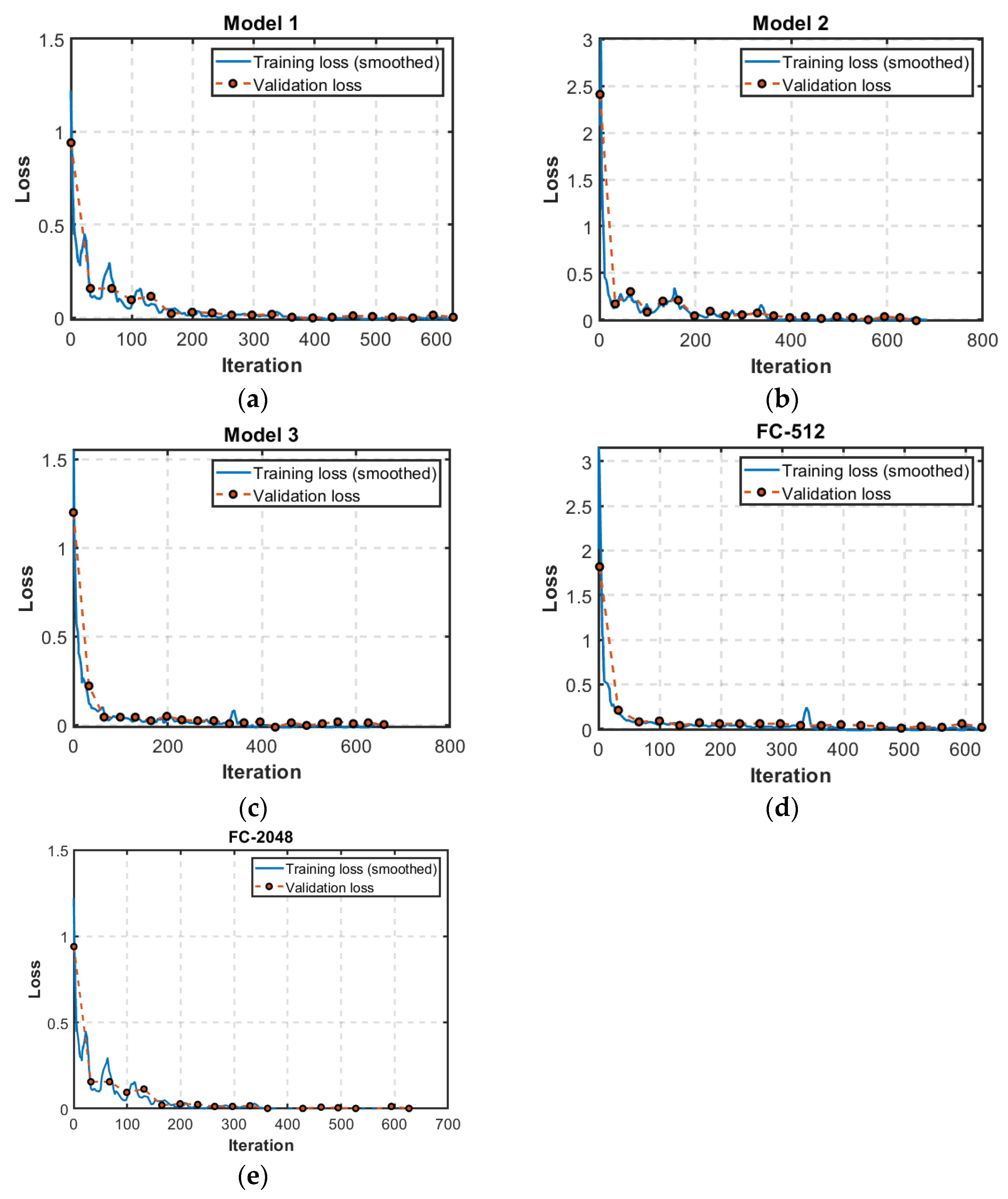
Figure 4 illustrates the loss function minimization process of CNN configurations to be evaluated. The solid line represents the smoothed training loss, and the red dots represent the loss of the validation set. The training process will be stopped if the validation loss satisfies the early stopping condition or the number of epochs reaches the maximum. The model will achieve better performance if the loss function finds a good local minim or a global minimum. From Figure 4, we can see that the training loss functions of all models are convergent to minimal loss. Similar results were obtained for every realization but are not included here for brevity.

4.1.2. Testing

After the training process, we tested CNNs with corresponding test sets. In this paper, the root-mean-square error was chosen to measure the error of CNN in DOA estimation. The results are shown in Table 3. Note that the CNN configuration with fewer stacked convolutional layers (Model 1) and fewer filters in the convolutional layer (Model 3) will lead to less time consumption but performs worse compared with Model 2. By comparing model FC-512, Model 2, and FC-2048, we found that the number of hidden units in a fully-connected layer has an effect on CNN performance. According to our experiment, more hidden units in a fully connected layer improves the prediction accuracy, but the computation time increases. In comparison, Model 2 can balance both estimation accuracy and computation time in the DOA estimation task. Therefore, in the following section, the CNN architecture of Model 2 was employed.

4.2. DOA Estimation Based on CNN

4.2.1. Model Training

After deciding on a certain CNN model, we utilized the simulated sea surface scattering datasets illustrated in the previous section to estimate DOA at different frequencies and wind speeds. Figure 5 shows the CNN configuration used for DOA estimation. Feature maps in Figure 5 represent the output of each average-pooling layer. The operating frequencies of the datasets are 5.3 GHz (at a wind speed of 25 m/s, 35 m/s, 45 m/s, and 55 m/s), 9.4 GHz (at wind speed of 5.5 m/s, 7.5 m/s, 12 m/s, 15 m/s, and 19.4 m/s), 13.9 GHz (same wind speeds as 9.4 GHz), and 13.99 GHz (at wind speed of 5 m/s, 10 m/s, 15 m/s, 20 m/s, 25 m/s, and 30 m/s). The implementation details are mentioned at the start of Section 4.1 and are not summarized here. The loss function is defined in Equation (14), and the optimizer to minimize the loss function is SGDM. Other training options were the same as an illustrated in Section 4.1. Similarly, we trained and tested the proposed CNN models with each dataset 100 times for a robust and stable result.

4.2.2. DOA Estimation Result

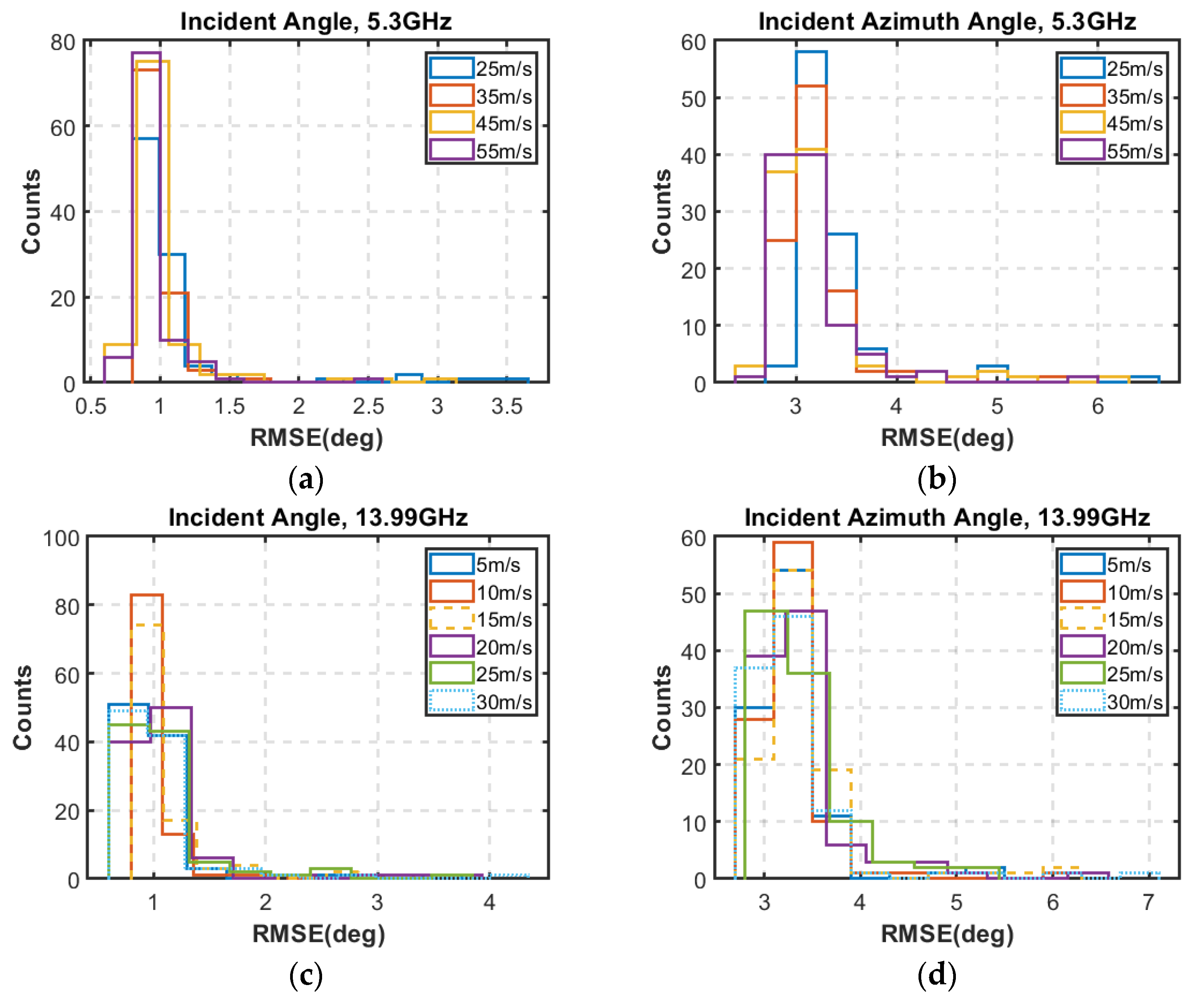
In this section, we evaluated the performance of Model 2 described in Figure 4. Table 2 summarizes the testing accuracy of DOA estimation-based sea surface scattering datasets at 5.3 GHz and 13.99 GHz. The values reported in this table are the average of 100 realizations. For incident angle estimation, the average RMSE of all datasets is about 1 , and for incident azimuth angle estimation, the average RMSE of all datasets is between 3 to 3.5 . For datasets at the 5.3 GHz operating frequency, we found that RMSE values of both the incident angle and incident azimuth angle are slightly decreased with increasing sea wind speed. However, for datasets under the 13.99 GHz operating frequency, there is no distinct relationship between RMSE and wind speeds. Figure 6 shows the distribution of RMSE between the truth and predicted incident source in 100 realizations. (a) and (b) are the RMSE distribution of θ i and ϕ i at 5.3 GHz and all wind speeds; (c) and (d) are the RMSE distribution of θ i and ϕ i at 13.99 GHz. The minimum RMSE of θ i and ϕ i in 100 realizations on 5.3 GHz, 25 m/s are 0.80 ° and 2.97 ° , on 35 m/s are 0.80 ° and 2.70 ° , on 45 m/s are 0.73 ° and 2.68 ° , and on 55 m/s are 0.76 °   and 2.67 ° . For 13.99 GHz, the minimum RMSE of θ i and ϕ i in 100 realizations on 5 m/s are 0.80 ° and 2.87 ° , on 10 m/s are 0.82 ° and 2.77 ° , on 15 m/s are 0.81 ° and 2.93 ° , on 20 m/s are 0.82 ° and 2.90 ° , on 25 m/s are 0.79 ° and 2.94 ° , and on 30 m/s are 0.78 ° and 2.74 ° . Besides, we added several samples consisting of measured data (Aquarius) and numerical model simulated data, and the network inversion are presented in Table 4.
Furthermore, we explored the CNN performance for datasets at the same wind speeds but different radar frequencies. Table 5 shows the average results of 100 realizations of the 9.4 GHz, 13.9 GHz, and 14.6 GHz datasets. For incident angle estimation, the average RMSE of all frequencies and wind speeds can approximately reach 1 . As for the incident azimuth angle, this value is dispersed from 3.24 to 3.52 . Figure 7 displays the distribution of RMSE of the 9.4 GHz, 13.9 GHz, and 14.6 GHz datasets. For 9.4 GHz, the minimum RMSE of θ i and ϕ i in 100 realizations on 5.5 m/s are 0.81 ° and 2.81 ° , on 7.5 m/s are 0.86 ° and 2.78 ° , on 12 m/s are 0.81 ° and 2.93 ° , on 15 m/s are 0.82 ° and 2.95 ° , and on 19.4 m/s are 0.82 ° and 2.85 ° . For 13.9 GHz, the minimum RMSE of θ i and ϕ i in 100 realizations on 5.5 m/s are 0.86 ° and 2.91 ° , on 7.5 m/s are 0.84 ° and 2.87 ° , on 12 m/s are 0.84 ° and 2.90 ° , on 15 m/s are 0.77 ° and 2.92 ° , and on 19.4 m/s are 0.80 ° and 2.94 ° . For 14.6 GHz, the minimum RMSE of θ i and ϕ i in 100 realizations on 5.5 m/s are 0.78 ° and 2.83 ° , on 7.5 m/s are 0.81 ° and 2.87 ° , on 12 m/s are 0.83 ° and 2.82 ° , on 15 m/s are 0.82 ° and 2.97 ° , and on 19.4 m/s are 0.81 ° and 2.88 ° .

4.2.3. Validation

In this paper, four types of validation data at the L-, C-, X-, and Ku-bands were adopted to examine the generalization ability of the proposed CNN structure. The L-band validation data for different wind directions come from the Aquarius scatterometer operating at 1.26 GHz, which has three incident angles from 28.7 ° to 45.6 ° . The backscattering coefficients from the sea surface are under 3, 5, 8, 10, 12, and 15 m/s wind speed [33,34]. The validation data for C- (5.3 GHz), X- (9.6 GHz), and Ku-bands (14 GHz) are generated by empirical CMOD7 [41], XMOD2 [42], and NSCAT-4 [43] models, respectively. Besides, other C- (5.3 GHz) and Ku-bands (13.9 GHz) data are radar measurements from [37] and [44], respectively. Due to the lack of bistatic scattering data, the scattering coefficients in a single validation sample are backscattered and mixed up with different frequencies and wind speeds. The incident angle and incident azimuth angle of the validation sample are 40 ° and 0 ° , respectively. Based on the above-mentioned validation data, the best prediction realized by the pre-trained CNN is 37.80 ° for the incident angle and 3.94 ° for the incident azimuth angle. As we can see, the estimation results of the mixed sample can achieve a satisfactory result.

5. Discussion

5.1. Results Interpretation

In our experiments, by comparing the average RMSE of all datasets listed in Table 4 and Table 5, we found that the performance of the CNN-based DOA estimation does not rely on radar frequencies and sea wind speeds. For almost all datasets, the average RMSE of incident angle is approaching 1 ° , and the average RMSE of the incident azimuth angle is between 3.0 ° and 3.5 ° . One possible reason is that the chosen CNN configuration is robust to the speckle noise appearing in coherent SAR measurements. Further investigation is required to generalize this claim.

5.2. Comparison with Other Algorithms

In this subsection, we compared the CNN-based method with the state-of-the-art DOA estimation algorithms, including machine learning or deep learning methods [13,45] and conventional parametric methods [46,47,48]. Those methods are proposed for local-scattered signal sources, which is quite similar to the sea surface scattering. The algorithms cited in this subsection process the signal sequence from the scattered sources, but in our case, the intensity of received signals was taken as the model input. The accuracy of the methods is summarized in Table 6. Using one-dimensional (1-D) DOA estimation means that only the incident angle was considered, while using the two-dimensional (2-D) DOA estimation, we predicted both the incident angle and incident azimuth angle of the signal sources. For 1-D DOA estimation, a machine learning-based approach, such as [45] utilizing the support vector machine (SVM), the RMSE of the incident angle was between 1 ° and 1.5 ° under the 7 dB of the signal to noise ratio (SNR). The authors of [46] used a multilayer perceptron neural network, and the RMSE of the DOA classifier was between 0.8 ° and 3 ° when 12.5% simulated training records were used (about 5895 samples in the dataset).
In [13], the authors proposed a deep neural network configuration for two signals in the presence of array imperfections, and the RMSEs were between 0.2 °   and 0.4 ° . Note that the local scattering angle was not considered in [13]. For 2-D DOA estimation, [47] used the ESPRIT-based method. The RMSE of the incident angle and incident azimuth angle in [47] was between 0.4 ° and 0.6 ° , 3 ° and 4 ° when the signal angular spreading degree was larger than 8 ° . In [48], the authors used the beamspace transformation method to estimate 2-D DOA. The RMSEs of the incident angle and incident azimuth angle were 0.7 ° and 1 ° , respectively, under 7 dB of SNR.
The accuracy in this paper is very close to the state-of-the-art signal processing-based works. Therefore, we can confirm that these results are quite satisfactory. We consider that using different deep learning techniques could lead to better results. For example, in [49], a Kalman filter-trained dynamic learning neural network (DLNN) was used to retrieve surface parameters from bistatic scattering data. Different from CNN, the configuration of DLNN is modified from multiple layer perceptron and each updated estimate of the DLNN weight is computed from the previous estimate and the new input data. The objective of [49] was to retrieve the surface parameters, while this paper was concerned with estimating the direction of the incident sources. Computationally, the sizes of input samples in [49] and in this work are also quite different.

5.3. Limitation

Perhaps, the biggest limitation of deep learning is its difficulty in generalization. Training a CNN to suit a variety of sea conditions and radar observations will lead to lower accuracy. Even though the observation in this article is omnidirectional, each dataset is still at a certain frequency and wind speed. Further investigation should ascertain the details of this trade-off between accuracy and generalization.
Another limitation is uncertainty. The existing uncertainty in these results is associated with the inaccuracy of speckle-interfered radar measurement modeling, sea surface roughness assumptions, and retrieval errors. We plan to compare the simulated data with real radar measurement data and use other deep learning models as a baseline algorithm in future work to reduce this error.

6. Conclusions

In this study, we present a novel method of two-dimensional DOA estimation for SAR systems based on sea surface scattering and convolutional neural networks. To simulate the bistatic radar measurement data of sea surface scattering under a certain operating frequency and sea wind speed, we utilized the AIEM model to calculate the bistatic scattering coefficients and then added a K-distributed bias as speckle noise in the real radar measurements. The radar operating frequencies used in this paper included C-band, X-band, and Ku-band, and the range of the sea wind speed was from 5 m/s to 55 m/s. We proposed a CNN structure that learns the characteristics of scattering pattern and strength both lengthwise and widthwise. In this way, CNN can make full use of the radar measurement data under different sea wind conditions to improve the estimation accuracy of the incident source. For each dataset, we trained and tested it 100 times. The experimental results showed that the CNN structure in Figure 5 could be applied on DOA estimation with satisfactory accuracy at a wide range of frequencies and sea wind speeds. The average RMSE of the incident angle is about 1 , and the average RMSE of the incident azimuth angle is between 3 and 3.5 .

Author Contributions

Conceptualization, K.-S.C. and Y.Y.; methodology, X.Z. and Y.Y.; software, X.Z.; validation, X.Z., Y.Y. and K.-S.C.; formal analysis, X.Z.; investigation, X.Z.; resources, X.Z.; data curation, X.Z.; writing—original draft preparation, X.Z.; writing—review and editing, K.-S.C. and Y.Y.; visualization, X.Z.; supervision, K.-S.C.; project administration, K.-S.C.; funding acquisition, K.-S.C. All authors have read and agreed to the published version of the manuscript.

Funding

This work was supported by the Guangxi Natural Science Youth Fund under Grant 2020GXNSFBA297105, and Guangxi Natural Science Fund for Innovation Research Team under Grant 2019GXNSFGA245001.

Conflicts of Interest

The authors declare no conflict of interest.

References

  1. Bartlett, M.S. Smoothing Periodograms from Time-Series with Continuous Spectra. Nature 1948, 161, 686–687. [Google Scholar] [CrossRef]
  2. Capon, J. High-Resolution Frequency-Wavenumber Spectrum Analysis. In Proceedings of the IEEE; IEEE: New York, NY, USA, 1969; pp. 1408–1418. [Google Scholar]
  3. Lacoss, R.T. Data Adaptive Spectral Analysis Methods. Geophysics 1971, 36, 661–675. [Google Scholar] [CrossRef]
  4. Schmidt, R.O. A Signal Subspace Approach to Multiple Emitter Location and Spectral Estimation. Ph.D. Thesis, Stanford University, Ann Arbor, MI, USA, 1982. [Google Scholar]
  5. Kumaresan, R.; Tufts, D.W. Estimating the Angles of Arrival of Multiple Plane Waves. IEEE Trans. Aerosp. Electron. Syst. 1983, AES-19, 134–139. [Google Scholar]
  6. Reddi, S.S. Multiple Source Location-A Digital Approach. IEEE Trans. Aerosp. Electron. Syst. 1979, AES-15, 95–105. [Google Scholar] [CrossRef]
  7. Barabell, A. Improving the Resolution Performance of Eigenstructure-based Direction-Finding Algorithms. In Proceedings of the ICASSP ’83-IEEE International Conference on Acoustics, Speech, and Signal Processing, Boston, MA, USA, 14–16 April 1983; pp. 336–339. [Google Scholar]
  8. DeGroat, R.D.; Dowling, E.M.; Linebarger, D.A. The Constrained MUSIC Problem. IEEE Trans. Signal Process. 1993, 41, 1445–1449. [Google Scholar] [CrossRef]
  9. Jha, S.; Durrani, T. Direction of Arrival Estimation Using Artificial Neural Networks. IEEE Trans. Syst. Man Cybern. Syst. 1991, 21, 1192–1201. [Google Scholar] [CrossRef]
  10. Southall, H.L.; Simmers, J.A.; Donnell, T.H.O. Direction Finding in Phased Arrays with a Neural Network Beamformer. IEEE Trans. Antennas Propag. 1995, 43, 1369–1374. [Google Scholar] [CrossRef]
  11. Rawat, A.; Yadav, R.N.; Shrivastava, S.C. Neural Network Applications in Smart Antenna Arrays: A Review. Int. J. Electron. Commun. 2012, 66, 903–912. [Google Scholar] [CrossRef]
  12. Terabayashi, K.; Natsuaki, R.; Hirose, A. Ultrawideband Direction-of-Arrival Estimation Using Complex-Valued Spatiotemporal Neural Networks. IEEE Trans. Neural Netw. Learn. Syst. 2014, 25, 1727–1732. [Google Scholar] [CrossRef]
  13. Liu, Z.; Zhang, C.; Yu, P.S. Direction-of-Arrival Estimation Based on Deep Neural Networks With Robustness to Array Imperfections. IEEE Trans. Antennas Propag. 2018, 66, 7315–7327. [Google Scholar] [CrossRef]
  14. Zooghby, A.H.E.; Christodoulou, C.G.; Georgiopoulos, M.A. Neural Network-based Smart Antenna for Multiple Source Tracking. IEEE Trans. Antennas Propag. 2000, 48, 768–776. [Google Scholar] [CrossRef]
  15. Valaee, S.; Champagne, B.; Kabal, P. Parametric Localization of Distributed Sources. IEEE Trans. Signal Process. 1995, 43, 2144–2153. [Google Scholar] [CrossRef]
  16. Lee, Y.U.; Lee, S.R.; Kim, H.M.; Song, I. Estimation of Direction of Arrival for Angle-Perturbed Sources. IEICE Trans. Fundam. Electron. Commun. Comput. Sci. 1997, E80A, 109–117. [Google Scholar]
  17. Astely, D.; Ottersten, B. The Effects of Local Scattering on Direction of Arrival Estimation with MUSIC. IEEE Trans. Signal Process. 1999, 47, 3220–3234. [Google Scholar] [CrossRef] [Green Version]
  18. Stoica, P.; Sharman, K.C. Maximum Likelihood Methods for Direction-of-Arrival Estimation. IEEE Trans. Acoust. Speech Signal Process. 1990, 38, 1132–1143. [Google Scholar] [CrossRef]
  19. Stoica, P.; Nehorai, A. MUSIC, Maximum Likelihood and Cramer-Rao Bound. In Proceedings of the ICASSP ’88-International Conference on Acoustics, Speech, and Signal Processing, New York, NY, USA, 11–14 April 1988; Volume 4, pp. 2296–2299. [Google Scholar]
  20. Stoica, P.; Nehorai, A. Performance Study of Conditional and Unconditional Direction-of-Arrival Estimation. IEEE Trans. Acoust. Speech Signal Process. 1990, 38, 1783–1795. [Google Scholar] [CrossRef]
  21. Tsakalides, P.; Nikias, C.L. Maximum Likelihood Localization of Sources in Noise Modeled as a Stable Process. IEEE Trans. Signal Process. 1995, 43, 2700–2713. [Google Scholar] [CrossRef]
  22. Ottersten, B.; Viberg, M.; Stoica, P.; Nehorai, A. Exact and Large Sample Maximum Likelihood Techniques for Parameter Estimation and Detection in Array Processing. In Radar Array Processing; Springer: Berlin/Heidelberg, Germany, 1993; pp. 99–151. [Google Scholar]
  23. Shan, T.J.; Wax, M.; Kailath, T. On Spatial Smoothing for Direction-of-Arrival Estimation of Coherent Signals. IEEE Trans. Acoust. Speech Signal Process. 1985, 33, 806–811. [Google Scholar] [CrossRef]
  24. Cai, B.; Li, Y.M.; Wang, H.Y. Forward/Backward Spatial Reconstruction Method for Directions of Arrival Estimation of Uncorrelated and Coherent Signals. IET Microw. Antennas Propag. 2012, 6, 1498–1505. [Google Scholar] [CrossRef]
  25. Dudczyk, J.; Kawalec, A. Adaptive Forming of the Beam Pattern of Microstrip Antenna with the Use of an Artificial Neural Network. Int. J. Antennas Propag. 2012, 2012. [Google Scholar] [CrossRef]
  26. Gierull, C.H. Ground Moving Target Parameter Estimation for Two-Channel SAR. IEEE Proc.-Radar Sonar Navig. 2006, 153, 224–233. [Google Scholar] [CrossRef]
  27. Gierull, C.H. Azimuth Positioning of Moving Targets in Two-Channel SAR by Direction-of-Arrival Estimation. Electron. Lett. 2004, 40, 1380–1381. [Google Scholar] [CrossRef]
  28. Fung, A.K.; Li, Z.; Chen, K.S. Backscattering from a Randomly Rough Dielectric Surface. IEEE Trans. Geosci. Remote. Sens. 1992, 30, 356–369. [Google Scholar] [CrossRef]
  29. Chen, K.S.; Wu, T.D.; Tsang, L.; Li, Q.; Shi, J.; Fung, A.K. Emission of Rough Surfaces Calculated by the Integral Equation Method with Comparison to Three-Dimensional Moment Method Simulations. IEEE Trans. Geosci. Remote. Sens. 2003, 41, 90–101. [Google Scholar] [CrossRef]
  30. Chen, K.S. Radar Scattering and Imaging of Rough Surfaces: Modeling and Applications with MATLAB@; CRC Press: Boca Raton, FL, USA, 2020. [Google Scholar]
  31. Chen, K.S.; Fung, A.K.; Weissman, D.A. A Backscattering Model for Ocean Surface. IEEE Trans. Geosci. Remote. Sens. 1992, 30, 811–817. [Google Scholar] [CrossRef]
  32. Xu, F.; Li, X.; Wang, P.; Yang, J.; Pichel, W.G.; Jin, Y. A Backscattering Model of Rainfall Over Rough Sea Surface for Synthetic Aperture Radar. IEEE Trans. Geosci. Remote. Sens. 2015, 53, 3042–3054. [Google Scholar] [CrossRef]
  33. Xie, D.F.; Chen, K.S.; Zeng, J.F. The frequency selective effect of radar backscattering from multiscale sea surface. Remote. Sens. 2019, 11, 160. [Google Scholar] [CrossRef] [Green Version]
  34. Xie, D.F.; Chen, K.S.; Yang, X.F. Effects of Wind Wave Spectra on Radar Backscatter from Sea Surface at Different Microwave Bands: A Numerical Study. IEEE Trans. Geosci. Remote. Sens. 2019, 57, 6325–6334. [Google Scholar] [CrossRef]
  35. Fung, A.K.; Chen, K.S. Microwave Scattering and Emission Models for Users; Artech House: Boston, MA, USA, 2010. [Google Scholar]
  36. Ulaby, F. Microwave Radar and Radiometric Remote Sensing; The University of Michigan Press: Chicago, IL, USA; Ann Arbor, MI, USA, 2014. [Google Scholar]
  37. Fung, A.K. Backscattering from Multiscale Rough Surfaces with Application to Wind Scatterometry; Artech House: Boston, MA, USA, 2015. [Google Scholar]
  38. Migliaccio, M.; Huang, L.; Buono, A. SAR Speckle Dependence on Ocean Surface Wind Field. IEEE Trans. Geosci. Remote. Sens. 2019, 57, 5447–5455. [Google Scholar] [CrossRef]
  39. Simonyan, K.; Zisserman, A. Very Deep Convolutional Networks for Large-Scale Image Recognition. In Proceedings of the International Conference on Learning Representations, San Diego, CA, USA, 7–9 May 2015. [Google Scholar]
  40. Liang, S.; Srikant, R. Why Deep Neural Networks for Function Approximation? In Proceedings of the International Conference on Learning Representations, Toulon, France, 24–26 April 2017.
  41. Stoffelen, A.; Verspeek, J.A.; Vogelzang, J.; Verhoef, A. The CMOD7 Geophysical Model Function for ASCAT and ERS Wind Retrievals. IEEE J. Sel. Top. Appl. Earth Obs. Remote. Sens. 2017, 10, 2123–2134. [Google Scholar] [CrossRef]
  42. Li, X.M.; Lehner, S. Algorithm for Sea Surface Wind Retrieval From TerraSAR-X and TanDEM-X Data. IEEE Trans. Geosci. Remote. Sens. 2014, 52, 2928–2939. [Google Scholar] [CrossRef] [Green Version]
  43. Royal Netherlands Meteorological Institute. NSCAT-4 Geophysical Model Function. Available online: http://knmi.nl/scatterometer/nscat_gmf (accessed on 1 May 2016).
  44. Schroeder, L.; Schaffner, P.; Mitchell, J.; Jones, W. AAFE RADSCAT 13.9-GHz Measurements and Analysis: Wind-Speed Signature of the Ocean. IEEE J. Ocean. Eng. 1985, 10, 346–357. [Google Scholar] [CrossRef]
  45. Pastorino, M.; Randazzo, A. A Smart Antenna System for Direction of Arrival Estimation Based on a Support Vector Regression. IEEE Trans. Antennas Propag. 2005, 53, 2161–2168. [Google Scholar] [CrossRef]
  46. Wen, C.; Shi, G.M.; Xie, X.M. Estimation of directions of arrival of multiple distributed sources for nested array. Signal Process. 2017, 130, 315–322. [Google Scholar] [CrossRef]
  47. Zheng, Z.; Li, G.J.; Teng, Y.L. Simplified Estimation of 2D DOA for Coherently Distributed Sources. Wirel. Pers. Commun. 2012, 62, 907–922. [Google Scholar] [CrossRef]
  48. Zheng, Z.; Wang, W.Q.; Meng, H.P.; So, H.C.; Zhang, H.B. Efficient Beamspace-Based Algorithm for Two-Dimensional DOA Estimation of Incoherently Distributed Sources in Massive MIMO Systems. IEEE Trans. Veh. Technol. 2018, 67, 11776–11789. [Google Scholar] [CrossRef]
  49. Yang, Y.; Chen, K.S.; Shang, G.F. Surface Parameters Retrieval from Fully Bistatic Radar Scattering Data. Remote. Sens. 2019, 11, 596. [Google Scholar] [CrossRef] [Green Version]
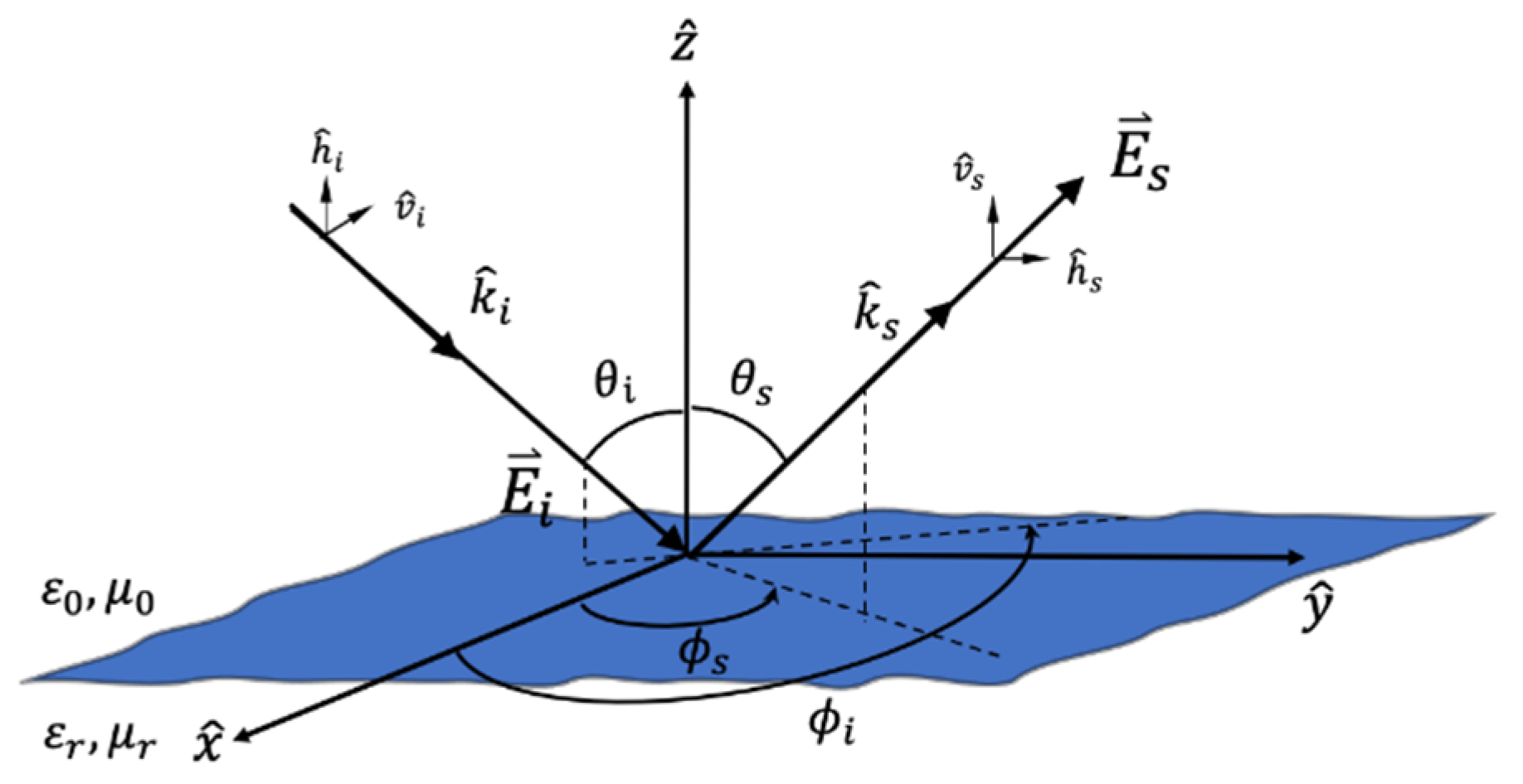
Figure 1. Geometry of the bistatic scattering from a sea surface.
Remotesensing 13 02681 g001
Figure 2. Hemispherical plots of bistatic scattering coefficients σ h h 0 , σ h v 0 , σ v h 0 , σ v v 0 with f = 5.3 GHz, U = 25 m/s, ϕ w = 30 : (a) ϕ i = 0 for all subplots; θ i = 20 for subplots in the left column and θ i = 60 for subplots in the right column; (b) θ i = 40 for all subplots; ϕ i for subplots in the left, middle, and right column are 30 , 90 , and 150 , respectively.
Remotesensing 13 02681 g002
Figure 3. Hemispherical plots of bistatic scattering coefficients σ h h 0 , σ h v 0 , σ v h 0 , σ v v 0 with θ i = 30 , ϕ i = 0 : (a) at 5.3 GHz operating frequency, U = 25 m/s; wind direction for subplots in the left and right columns is up/downwind (0°/180°) and crosswind (90o), respectively (b) at 13.9 GHz, ϕ w = 30 and U = 7.5 m/s for left-row subplots.
Remotesensing 13 02681 g003
Figure 4. Loss function minimization process of five different CNN configurations: (a) Model 1; (b) Model 2; (c) Model 3; (d) FC-512; (e) FC-2048. The experiment is based on the simulated sea surface scattering dataset at 13.9 GHz, 5.5 m/s.
Remotesensing 13 02681 g004
Figure 5. The CNN configuration employed for DOA estimation. The network is consisted of 10 convolutional layers, 4 average pooling layers, and a fully connected layer with 1024 hidden units.
Remotesensing 13 02681 g005
Figure 6. The distribution of RMSE between the truth and predicted incident source for datasets at 5.3 GHz and 13.99 GHz in 100 realizations: (a) 5.3 GHz, incident angle; (b) 5.3 GHz, incident azimuth angle; (c) 13.99 GHz, incident angle; (d) 13.99 GHz, incident azimuth angle.
Remotesensing 13 02681 g006
Figure 7. The distribution of RMSE between the truth and predicted incident source for datasets at 13.9 GHz and 14.6 GHz in 100 realizations: (a) 9.4 GHz, incident angle; (b) 9.4 GHz, incident azimuth angle(c) 13.9 GHz, incident angle; (d) 13.9 GHz, incident azimuth angle; (e) 14.6 GHz, incident angle; (f) 14.6 GHz, incident azimuth angle.
Remotesensing 13 02681 g007
Table 1. The ranges of the incidence and received angle, operating frequencies, and sea wind speeds in the DOA estimation experiment.
ParametersDescriptionRangeStep Size
θ i Incident angle 20 70 5
ϕ i Incident azimuth angle 10 170 5
θ s Scattering angle 10 70 5
ϕ s Scattering azimuth angle 10 170 5
ϕ w Wind direction 0 180 5
f Frequency5.3 GHz/9.4 GHz/13.9 GHz/13.99 GHz/14.6 GHz
U Wind speed25 m/s–55 m/s (5.3 GHz)
5 m/s–30 m/s (13.99 GHz)
5.5 m/s–19.4 m/s (9.4 GHz, 13.9 GHz,14.6 Hz)
10 m/s (5.3 GHz)
5 m/s (13.99 GHz)
Table 2. CNN configurations (shown in columns). The depth of the configurations increases from the left (Model 1) to the right (Model 2), as more layers are added. Besides, the number of filters decreases from Model 2 to Model 3. Changes are shown in bold. The aim of model “FC-512” and “FC-2048” is to compare the performance between models with different numbers of hidden units in the fully connected layer. The convolutional layer is abbreviated as “Conv” and layer parameters are denoted as “length × width × number of filters, stride”. The average-pooling layer is abbreviated as “Avg-p” and layer size is denoted as “length × width, stride”. “FC” and “Regrs” represent a fully connected layer and a regression layer, respectively.
Model 1Model 2Model 3FC-512FC-2048
Layer TypeSizeLayer TypeSizeLayer TypeSizeLayer TypeSizeLayer TypeSize
Input 1221 × 6 × 1Input1221 × 6 × 1Input1221 × 6 × 1Input1221 × 6 × 1Input1221 × 6 × 1
Conv1 × 2 × 32, 2Conv1 × 2 × 32, 2Conv1 × 2 × 16, 2Conv1 × 2 × 32, 2Conv1 × 2 × 32, 2
Conv1 × 3 × 32Conv1 × 3 × 32Conv1 × 3 × 16Conv1 × 3 × 32Conv1 × 3 × 32
Conv5 × 1 × 64Conv 5 × 1 × 64Conv5 × 1 × 32Conv5 × 1 × 64Conv5 × 1 × 64
Conv5 × 1 × 64Conv5 × 1 × 64Conv5 × 1 × 32Conv5 × 1 × 64Conv5 × 1 × 64
Avg-p6 × 1, 2Avg-p6 × 1, 2Avg-p6 × 1, 2Avg-p6 × 1, 2Avg-p6 × 1, 2
Conv7 × 1 × 128Conv7 × 1 × 128Conv7 × 1 × 64Conv7 × 1 × 128Conv7 × 1 × 128
Conv7 × 1 × 128Conv7 × 1 × 128Conv 7 × 1 × 64Conv7 × 1 × 128Conv7 × 1 × 128
Avg-p8 × 1, 2Avg-p8 × 1, 2Avg-p8 × 1, 2Avg-p8 × 1, 2Avg-p8 × 1, 2
Conv9 × 1 × 256Conv9 × 1 × 256Conv9 × 1 × 128Conv9 × 1 × 256Conv9 × 1 × 256
Avg-p10 × 1, 2Avg-p10 × 1, 2Avg-p10 × 1, 2Avg-p10 × 1, 2Avg-p10 × 1, 2
FC1024Conv11 × 1 × 512Conv11 × 1 × 256Conv11 × 1 × 512Conv11 × 1 × 512
Regrs2Conv11 × 1 × 512Conv11 × 1 × 256Conv11 × 1 × 512Conv11 × 1 × 512
Avg-p12 × 1, 2Avg-p12 × 1, 2Avg-p12 × 1, 2Avg-p12 × 1, 2
FC1024FC1024FC512FC2048
Regrs2Regrs2Regrs2Regrs2
Table 3. Performance of 100 realizations of the dataset at 13.9 GHz, 5.5 m/s using the CNN methods illustrated in Table 2. The numbers reported in this table are the average of all realizations.
Model 1Model 2Model 3FC-512FC-2048
Time Consuming (sec)315425175389621
RMSE of Incident Azimuth Angle3.89 ° 3.31 ° 4.39 ° 4.55 ° 3.13 °
RMSE of Incident Angle1.04 ° 1.05 ° 1.14 ° 1.11 ° 1.01 °
Table 4. Results of 100 realizations of the 5.3 GHz and 13.99 GHz datasets using the CNN method illustrated in Figure 5. The numbers reported in this table are the average of all realizations.
f U RMSE   of   θ i RMSE   of   ϕ i
5.3 GHz25 m/s 1.13 3.37
35 m/s 0.98 3.20
45 m/s 0.96 3.18
55 m/s 0.94 3.16
13.99 GHz5 m/s 1.05 3.31
10 m/s 1.03 3.27
15 m/s 1.09 3.40
20 m/s 1.11 3.37
25 m/s 1.11 3.42
30 m/s 1.05 3.30
Table 5. Results of 100 realizations of the 9.4 GHz, 13.9 GHz, and 14.6 GHz datasets using the CNN method illustrated in Figure 5. The numbers reported in this table are the average of all realizations.
f U RMSE   of   θ i RMSE   of   ϕ i
9.4 GHz5.5 m/s 1.06 3.30
7.5 m/s 1.04 3.25
12 m/s 1.05 3.37
15 m/s 1.03 3.36
19.4 m/s 1.04 3.30
13.9 GHz5.5 m/s 1.04 3.33
7.5 m/s 1.01 3.26
12 m/s 1.03 3.32
15 m/s 1.08 3.52
19.4 m/s 1.00 3.36
14.6 GHz5.5 m/s 0.98 3.27
7.5 m/s 1.04 3.28
12 m/s 0.98 3.24
15 m/s 1.01 3.35
19.4 m/s 1.00 3.24
Table 6. The accuracy of other state-of-the-art signal processing-based DOA estimation algorithms.
Algorithms RMSE   of   θ i RMSE   of   ϕ i
1-D DOA estimationSVM [45]1 ° –1.5 ° ---
Annihilating filter with structured low rank approximation technique [46]0.8 ° –3 °
DNN [47]0.2 ° –0.4 °
2-D DOA estimationESPRIT-based method [48]0.4 ° –0.6 ° 3 ° –4 °
Beamspace transformation [49]0.7 ° 1 °
Publisher’s Note: MDPI stays neutral with regard to jurisdictional claims in published maps and institutional affiliations.