Abstract
Accurate and timely detection of phenology at plot scale in rice breeding trails is crucial for understanding the heterogeneity of varieties and guiding field management. Traditionally, remote sensing studies of phenology detection have heavily relied on the time-series vegetation index (VI) data. However, the methodology based on time-series VI data was often limited by the temporal resolution. In this study, three types of ensemble models including hard voting (majority voting), soft voting (weighted majority voting) and model stacking, were proposed to identify the principal phenological stages of rice based on unmanned aerial vehicle (UAV) RGB imagery. These ensemble models combined RGB-VIs, color space (e.g., RGB and HSV) and textures derived from UAV-RGB imagery, and five machine learning algorithms (random forest; k-nearest neighbors; Gaussian naïve Bayes; support vector machine and logistic regression) as base models to estimate phenological stages in rice breeding. The phenological estimation models were trained on the dataset of late-maturity cultivars and tested independently on the dataset of early-medium-maturity cultivars. The results indicated that all ensemble models outperform individual machine learning models in all datasets. The soft voting strategy provided the best performance for identifying phenology with the overall accuracy of 90% and 93%, and the mean F1-scores of 0.79 and 0.81, respectively, in calibration and validation datasets, which meant that the overall accuracy and mean F1-scores improved by 5% and 7%, respectively, in comparison with those of the best individual model (GNB), tested in this study. Therefore, the ensemble models demonstrated great potential in improving the accuracy of phenology detection in rice breeding.
1. Introduction
In rice breeding, the accurate phenological information of rice is essential for breeders to make decisions in fertigation and breeding operations accordingly [1]. Crop phenological stages have a close relationship with climate conditions [2], but are also affected by genetic variability [3]. Traditionally, the approach of detecting crop phenology uses visual observations to identify the timing of periodic events such as germination, flowering, and physiological maturity [1,4]. However, field observation is indeed time-consuming and labor-intensive work which is often constrained by the observer’s subjective perception of the canopy status [5].
As an alternative method, remote sensing data based on satellites has been successfully used to detect landscape-scale phenology [2,6,7,8]. Landsat was firstly used to characterize the seasonal changes of vegetation at regional scales [9]. However, some plant phenological stages changed rapidly, which limited the application of Landsat due to its long revisit time (16 days). Since the Moderate Resolution Imaging Spectrometer (MODIS) was launched, it provided time-series vegetation indices (VIs) with a high temporal (daily) and medium spatial resolution (250–500 m) [7]. Many previous studies have exploited the MODIS data to detect the phenological variation of different crops including maize [7], wheat [10,11] and rice [12,13,14], as well as other crops [15,16,17]. In addition, some studies retrieved plant phenology from fine resolution satellite imagery based on new optical sensors [18]. Pan et al. [6] constructed a time-series NDVI dataset from HJ-1 A/B and found that the crop season start or end from HJ-1 A/B imagery was comparable with local observations. Vrieling et al. [18] mapped the spatial distribution of vegetation phenology at 10 m resolution derived from Sentinel-2A. However, the application of satellite-optical sensors has still been challenged as a method of phenology retrieval due to the risk of poor data quality as a result of clouds [19]. Synthetic Aperture Radar (SAR) satellites without the limitation of weather conditions have been applied to derive vegetation morphological and phenological information [20]. Fikriyah et al. [21] used temporal information based on SAR backscatter to monitor the differences in rice growth. He et al. [22] found that the backscattering parameters from RADARSAT-2 had a strong correlation with rice phenology in a study in Meishan, China. Although the regional or global distributions of vegetation phenology can be retrieved from satellite sensors, these are not capable of properly detecting phenological variability of small-size farmland and crop breeding due to the limitation of high temporal and spatial resolution [1,4,23].
Compared to the satellites, the imagery from digital cameras for near-surface observations had a higher temporal and spatial resolution [24]. Especially, the consumer-grade cameras with RGB (R, G, B) bands mounted on unmanned aerial vehicles (UAV) are cost-effective and flexible to revisit fields to collect time-series images during the vegetation growing season [4]. Park et al. [25] used RGB images from UAV with a machine learning method to assess leaf phenology of trees and highlighted the feasibility of texture characteristics for phenological analysis in tropical forest. Burkart et al. [26] calculated the time-series Green-Red Vegetation Index (GRVI) from UAV-RGB imagery and analyzed its potential to track seasonal changes of barley. Yang et al. [4] constructed a deep learning approach to identify principal phenology of rice from a mono-temporal UAV imagery. These preliminary studies have proven the feasibility of tracking vegetation phenology based on UAV imagery with various working principles.
By reviewing the previous studies in the literature, the common methodologies of phenology acquisition from satellite or near-surface images are mainly shown as three types: (1) curve fitting methods which used logistic function, Gaussian function and Savitzky–Golay filtering to smooth the VI’s time-series curves and then extracted phenology based on its inflection points [27,28,29]; (2) shape model fitting (SMF) methods which smoothed VI data and extracted phenological stages based on optimum scaling parameters and visual observations [7,24]; (3) machine learning or deep learning algorithms which fed VIs, textures or images into models to estimate phenological stages [4,25]. The first two types of methods highly relied on the amount of time-series image data and neglected the heterogeneity of crops’ annual growth progress [4,24]. Since the advance of computing power and neural network algorithms, many studies have successfully used deep learning techniques to estimate vegetation parameters [30,31,32,33]. However, the large amount of reference data for deep learning is still a challenge for scientists. In contrast, machine learning has no high requirements for computer hardware configuration and amount of datasets. Therefore, machine learning has great potential to reconstruct time-series datasets and detect phenology [24]. In recent years, ensemble machine learning models based on a combination of individual models have been proved to be more effective at making predictions [34,35]. Shahhosseini et al. [36] combined linear, least absolute shrinkage and selection operator (LASSO), eXtreme Gradient Boosting (XGBoost), Light Gradient Boosting Machine (LightGBM) and random forests (RF) to forecast corn yield. Masiza et al. [37] combined XGBoost with support vector machine (SVM), artificial neural network (ANN), naïve Bayes (NB) and RF to map landscape in a smallholder farming system. Although some ensemble methods have been applied in agriculture domain, to the best of our knowledge, the performance and potential of different ensemble models are rarely compared and tested for detecting phenology.
In this study, our main research problem is as follows: is UAV-RGB imagery sufficient to accurately identify phenology in heterogeneous rice? Moreover, given the recent introduction of ensemble algorithms into phenological extraction, little is known about whether ensemble models could improve the accuracy in phenological detection compared to machine learning models. Based on the above-mentioned question, firstly, the high-resolution imagery from UAV-RGB images was used to calculate VIs and textures in the plot level. Then, three model ensemble methods (soft voting, hard voting and model stacking) based on five machine learning algorithms (k-nearest neighbors, Gaussian naïve Bayes, logistic regression, RF and SVM) were the first time to be used to detect rice phenology in breeding trials. Accordingly, the objectives of the study are: (1) to build the ensemble models to detect rice phenology, (2) to compare the performance of the machine learning models and ensemble models for detecting phenology, and (3) to analyze the contributions of feature variables in the ensemble models.
2. Materials and Methods
2.1. Study Area
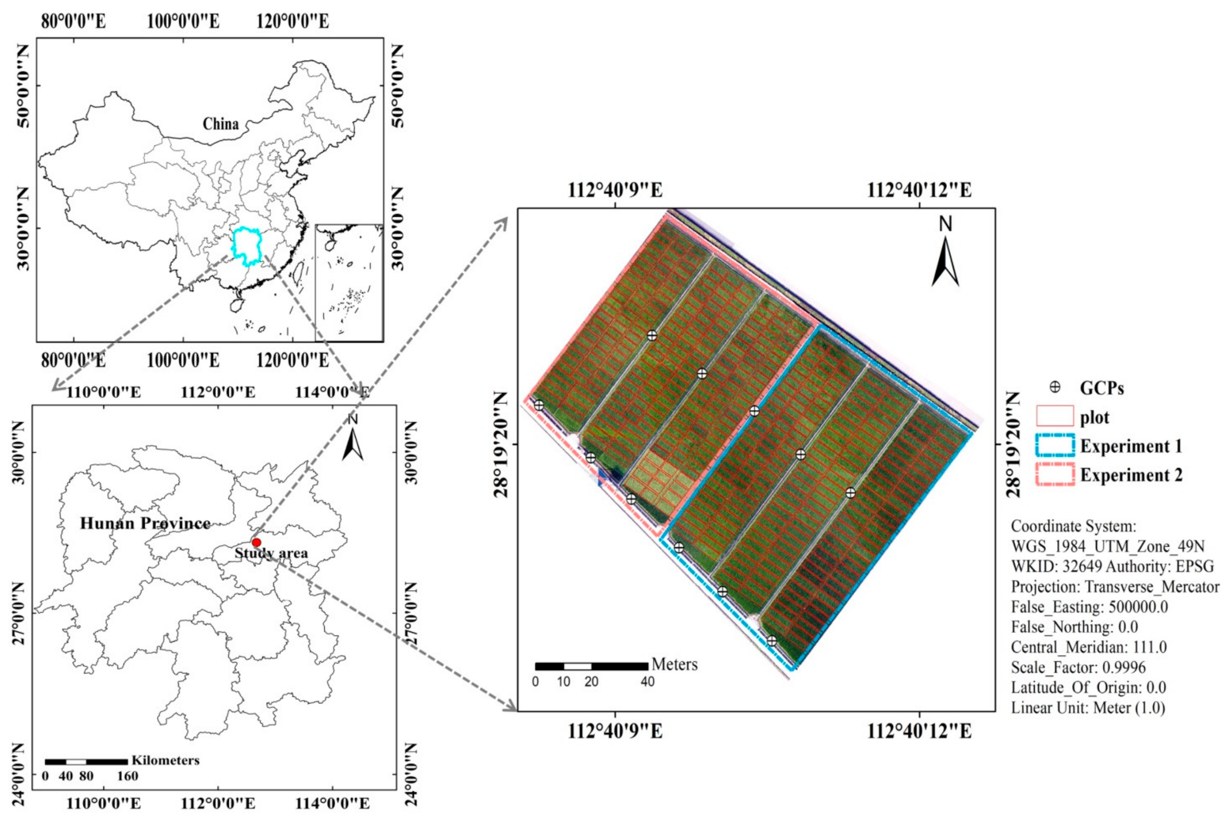
The breeding trails were carried out at the Guanshan rice breeding base (28°19′ N, 112°40′ E), Jinzhou town, Ningxiang district, Changsha city, Hunan Province, China (Figure 1). The annual average rainfall was 1358 mm. Average daily temperature was 16.8 °C. The average daily sunshine hour duration is about 4.8 h. There are two hybrid rice experiments in the study area. Experiment 1 was designed with late-maturity cultivars and sowing date was 18 June 2020. Experiment 2 was designed with early-medium-maturity cultivars which were sowed at 22 June 2020. The experimental field was divided into 437 plots in total. Each cultivar was transplanted into an individual plot. Among these plots, 279 plots and 158 plots were the same sizes of 2.5 × 5 m and 2.5 × 7.5 m, respectively. The same N and irrigation treatment was applied for all plots. Eleven ground control points (GCPs) were distributed across the field (Figure 1). These points were obtained from a Hiper Topcon DGPS (Topcon Co., Ltd., Tokyo, Japan) with 0.01 m vertical and horizontal precision.

Figure 1.
The location of the study area in Changsha City, Hunan Province, China (Experiment 1: late-maturity cultivars, Experiment 2: early-medium-maturity cultivars).
2.2. Field-Based Observations of Rice Phenology
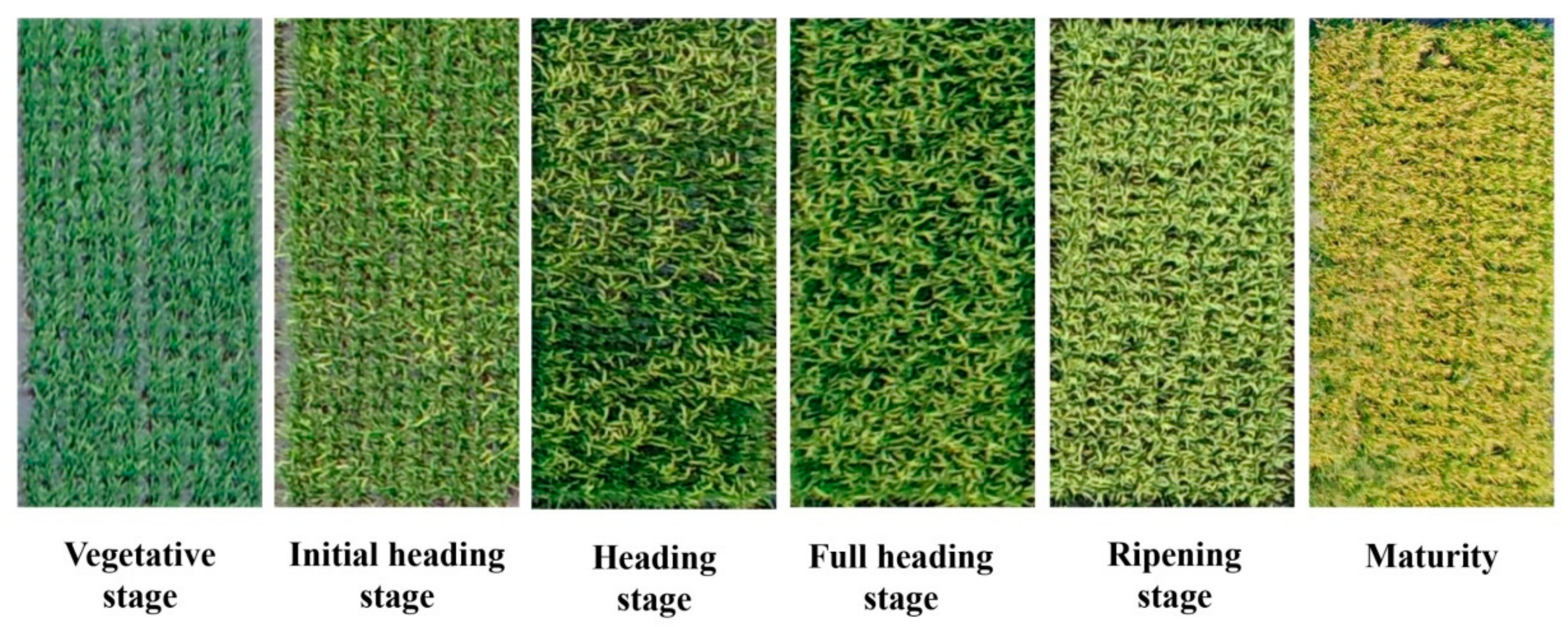
In the field survey, rice breeders observed and recorded the phenological stages of the different cultivars during rice growing season. In this study, the vegetative phase, initial heading stage, heading stage, full heading stage, ripening phase and maturity were collected (Figure 2). The detailed descriptions of these phenological stages were presented by Fageria [38] and Yang et al. [4].
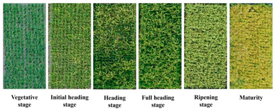
Figure 2.
Detailed overview of the rice’s main phenological stages derived from UAV-RGB imagery at the flight altitude of 50 m above the ground.
2.3. Image Prepocessing
2.3.1. Images Collection
The UAV used in this paper was a four-rotor consumer-grade UAV called Phantom 4 Pro (DJI Technology Co., Ltd., Shenzhen, China) which was equipped with a RGB camera offering a spatial resolution of 20-mega pixels. A lens of 35 mm focal length was mounted on the RGB camera which could acquire an image with 5456 × 3632 pixels in a short period of time (faster than 1/2000 s). The flight duration of the UAV was about 30 min. During rice growing season, five flights were carried out between August and November in 2020. The detailed information of flights is shown in Table 1. The UAV was flown at the flight altitude of 50 m above ground for each flight, resulting in the ground sampling distance of 1.36 cm. At each flight, Pix4Dcapture software was used to set the flight waypoints. This resulted in the flight speed of 2.8 m/s, forward overlap of 80% and side overlap of 70%. In addition, the flights were conducted on the stable ambient light between 11:00 am and 13:00 pm [39].

Table 1.
Dates of the UAV flights and statistical numbers of plots in main phenological stages for each flight.
2.3.2. Generation of Orthomosaic Maps
After each flight, the RGB images of the experimental plots were downloaded from the SD card. Generating orthomosaic maps requires one to (1) align raw images; (2) georeference images—11 GCPs were imported, placed manually on one image and automatically projected to the remaining images [40]; and (3) export the orthomosaic maps with TIFF-image format. In this study, Pix4Dmapper 1.1.38 (Pix4D SA, Lausanne, Switzerland) was used to carry out the above-mentioned steps to generate orthomosaic maps. The radiance reaching the camera had an empirical linear relationship with digital numbers (DN) in each band; therefore, linear equations which were introduced by Yu et al. [41] can be carried out to maintain radiometric consistency of multi-temporal images. The images taken on August 1 were used as the reference images; normalization coefficients for images taken at subsequent dates were calculated and applied to the orthomosaic maps to accomplish radiometric normalization.
2.3.3. Calculation of VIs or Color Space
The VIs or color space were calculated from the DN values of the UAV-RGB imagery (see Table 2). Firstly, ArcGIS v.10.0 (ESRI, Redlands, CA, USA) was used to generate regions of interest (ROIs) by manually delineating plots in orthomosaics (Figure 1). Secondly, the selected VIs or color space were extracted based on the R, G, B bands of orthomosaic maps by using Python 3.6. Then, the mean VIs or bands of ROI were calculated by using the “ZonalStatisticsAsTable” module in ArcGIS v.10.0 software.
Table 2.
Descriptions of VIs or color space derived from UAV-RGB imagery.
2.3.4. Calculation of Texture Features
The methodology of gray level co-occurrence matrix (GLCM) was proposed by Haralick et al. [47] for characterizing the heterogeneity and inhomogeneity of images. GLCM highlights texture properties, such as homogeneity, contrast or irregularity. Texture was the term which was used to characterize the tones of gray-level variations in digital images [48]. The construction of GLCM firstly converted an image to grayscale to be discretized in the whole matrix. The method was to divide the range of continuous pixel values into N sub samples of equal width, called gray level, and then remap these values on a single gray level. Based on the discretized mapping, the elements of GLCM were obtained by calculating the frequency of pixel pairs with specific gray levels and spatial relationship in the matrix. Many previous studies have successfully extracted GLCM from UAV-based imagery to estimate crop parameters [49,50,51]. In this study, ENVI 5.3 (Harris Geospatial Solutions, Inc., Broomfield, CO, USA) was applied to calculate eight textures (mean, variance, contrast, homogeneity, dissimilarity, correlation, entropy and second moment). To calculate the texture for each pixel, a 3 × 3 window size as a moving window was used to obtain statistics. This selected window size could capture small differences between pixel values in small extents [52]. After calculation of GLCM, the ArcGIS v.10.0 software was used to obtain the mean of each texture for each plot.
2.4. Classifier Techniques
2.4.1. Multiple Machine Learning Algorithms
Five machine learning classification algorithms were selected to detect phenology in rice breeding. These algorithms are including RF, k-nearest neighbors (KNN), Gaussian naïve Bayes (GNB), support vector machine (SVM) and logistic regression (LR). All the user-defined parameters from the five different types of classifiers were determined by “GridSearchCV” method with 10-fold cross validation in Python 3.6 environment (Table A1). Brief descriptions of the selected algorithms are in the following paragraphs.
RF is a widely used machine learning algorithm which was developed by Breiman [53]. RF was created based on the combination with a set of decision trees. The classification results of RF were determined by majority voting of trees. In this study, RF has two parameters to be tuned including “max_depth” (the maximum depth of trees) and “n_estimators” (the number of trees in the forest). The “RandomForestClassifier” function in “sklearn” package was used to implement RF.
KNN is a well-known machine learning method for classification [54]. The basic idea of this algorithm is that most of the K similar samples (neighbors) in the feature space belong to a certain category, and then the sample belongs to this category. The classifiers of samples were determined by the category of the nearest one or several samples. For this study, only one parameter defined by the user, “n_neighbors” (number of neighbors) needs to be tuned in “sklearn” package.
GNB was one of simple fast classification algorithms, which was usually suitable for datasets with high dimensions [55]. Because of its fast running speed and few tuning parameters, it is very suitable to provide fast, robust and automated results for classification [55]. In this paper, default parameters were used to train the GNB model.
SVM used a kernel learning method to classify data, even if the data are not linearly separable [56]. For the nonlinear problems, the method of SVM is to select the kernel function and map the training samples to the high-dimensional space through the kernel function, so as to obtain the best hyperplane in the high-dimensional space. The advantage of using the kernel function is that the computation is not much more complex than before while obtaining the optimal hyperplane [54,57]. Compared with other traditional learning algorithms, the SVM algorithm can effectively avoid the problems of local optimal solution and dimension disaster. In this work, two user-defined parameters including “C” (the strength of the regularization) and “kernel” (the kernel type) were tuned.
LR is a widely accepted algorithm which can deal with binary or multiclass problems [58]. In this study, the “LogisticRegression” function in the “sklearn” package was used to obtain the LR model. The LR algorithm was applied with three user-defined parameters including “C” (inverse of regularization strength), “penalty” (specify the norm used in the penalization) and “solver” (the class implements regularized logistic regression).
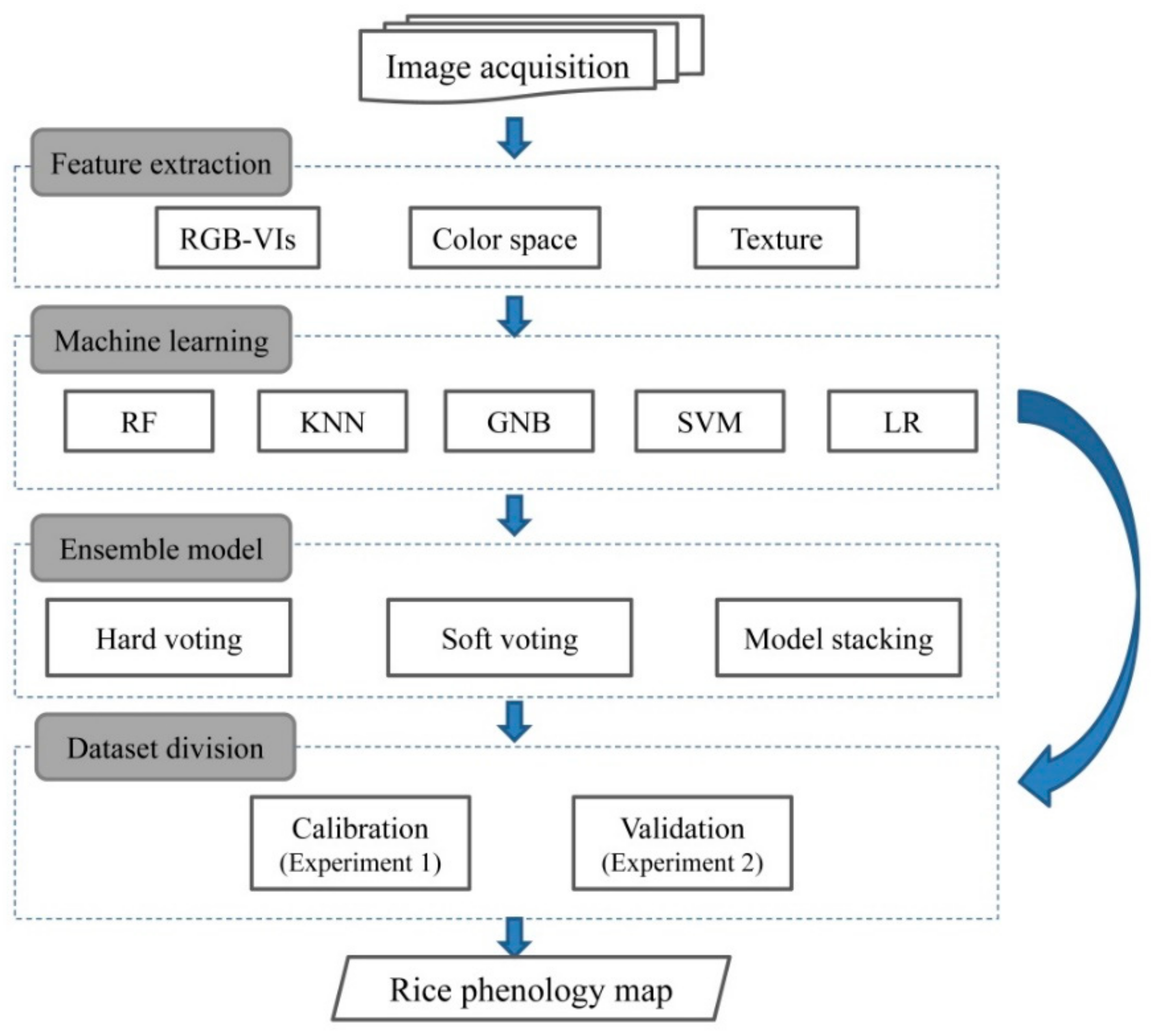
2.4.2. Ensemble Models
The primary goal of using ensemble models is to reduce the risk of selecting a classifier with poor performances, or improve the accuracy of an individual classifier [59]. In this study, three ensemble strategies, namely hard voting, soft voting and model stacking were used to create ensemble models (Figure 3). In the case of hard voting, the output of the ensemble model is the most assigned class by multiple classifiers. In the soft voting rule, a weight was assigned to individual classifier to favor classifiers with better performance in voting decision. Model stacking takes predictions generated by multiple classifiers and uses these predictions as inputs in a second-level learning classifier.
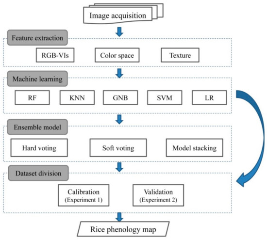
Figure 3.
Schematic diagram of the proposed methods.
The hard voting rule of an ensemble model on decision problem works as follows:
where is the selected class number of hard voting on decision problem . is the number of voters (base classifiers). is the binary vector output (e.g., [0, …, 0, 1, 0, …, 0]) of the classifier on the decision problem . is the index where the maximum value was obtained in the summation vector . If multiple maximum values were found, the index of first occurrence is returned.
For the soft voting, the classifiers with good performances were assigned larger weights. The soft voting is an extension of the Equation (1) and uses weights per base machine learning classifier .
where is the kappa coefficient of the classifier over the independent sample set [60].
Model stacking is an ensemble algorithm that assembles RF, KNN, GNB, SVM and LR methods. According to this method, a higher level (level 2) meta-model is trained on the predictions of base models (level 1); then, a final output of the overall ensemble model is generated [61]. In this study, five machine learning models were used as the level-1 models and GNB as the level-2 model.
2.5. Evaluation of Model Accuracy
In order to evaluate the performance of different machine learning classifiers and ensemble models for phenology detection, several strategies were carried out. Firstly, the accuracy of each machine learning algorithm was tested. Secondly, the proposed ensemble models based on five individual machine learning classifiers were conducted for detecting rice phenology. Then, the ensemble models were compared with the result of the best individual classifier model. Finally, the phenological maps in rice breeding produced by the optimal model were visually evaluated.
In this study, the data from Experiment 1 were selected to train the estimation models, and the independent data from Experiment 2 were used to validate these models. The assessment of models was carried out on the six principal phenological stages: vegetative stage, initial heading stage, heading stage, full heading stage, ripening stage and maturity stage. Two metrics were selected to evaluate the accuracies of classifiers: overall accuracy and F1-score. These two metrics are calculated as follows:
where , , , and in Equation (4) represent True Positive, True Negative, False Positive, False Negative and a total number of items, respectively. The confusion matrixes were used to show the distribution of omission and commission errors across different phenological stages. In addition, the “feature_importance_permutation” function in “mlxtend” package was used to evaluate the feature importance of ensemble models in Python 3.6 running environment.
3. Results
3.1. Variation of Observed Phenology in Different Plots
Figure 4 shows the statistical distributions of observed main phenology in different plots. Although there was a four-day difference in sowing dates between Experiment 1 and Experiment 2, all plots had the same transplanting date (13 July 2020). Due to the variance of cultivar traits, the phenology was highly heterogeneous in different plots. The dates of phenology in early-medium-maturity cultivars were earlier than those in late-maturity cultivars. The mean dates of initial heading, full heading and maturity stages in Experiment 1 are September 8 (DOY = 252), September 14 (DOY = 258) and November 11 (DOY = 306), respectively. The mean dates of corresponding phenology in Experiment 2 are September 4 (DOY = 248), September 10 (DOY = 254) and October 26 (DOY = 300), respectively.
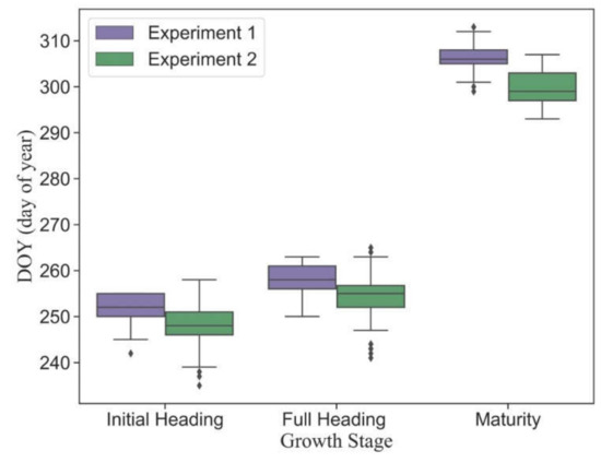
Figure 4.
The statistical distribution of the main observed phenology in Experiment 1 (late-maturity cultivars) and Experiment 2 (early-medium-maturity cultivars).
3.2. Model Performance by Multiple Machine Learning
Five machine learning algorithms, including RF, KNN, GNB, SVM and LR, were investigated to compare the performance for phenological detection. In the calibration dataset, RF performed best among these machine learning models (overall accuracy = 93% and mean F1-score = 0.84). Other models produced comparable accuracies, resulting in overall accuracies from 85% to 88% and mean F1-scores from 0.73 to 0.77 (Figure 5). For individual phenology, all models had good performance for detecting vegetative, ripening and maturity stages and resulted in F1-scores from 0.81 to 1.0 (Table 3). However, these models obtained slightly worse accuracies for phenological detection at initial heading, heading and full heading stages. Accordingly, the F1-scores ranged from 0.39 to 0.79.
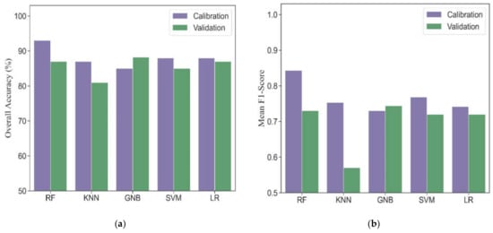
Figure 5.
The overall accuracies (a) and mean F1-scores (b) in different machine learning models for phenological detection in calibration and validation datasets.
Table 3.
The F1-scores of different machine learning models for detecting phenology in calibration and validation datasets.
In the validation dataset, the GNB model obtained the most accurate estimation with overall accuracy of 88% and mean F1-socre of 0.74. The RF, LR and SVM models had similar performance with overall accuracies ranging from 85% to 87%, and mean F1-scores ranging from 0.72 to 0.73. The KNN model yielded the worst performance (overall accuracy = 81% and mean F1-score = 0.57). Except for the KNN model, other models tested in the validation dataset showed consistency with those in the calibration dataset for detecting vegetative, ripening and maturity stages (F1-scores from 0.83 to 0.98). The transition dates of initial heading, heading and full heading are close to each other. It is challenging for all models to accurately identify these phenological stages. Thus, the F1-scores of different machine learning models at heading phase were lower than those at other phenological stages and ranged from 0.44 to 0.65 except for KNN.
3.3. Model Performance by Ensemble Models
Three different strategies of ensemble models based on base classifiers (five machine learning models) were investigated to evaluate the performances for phenological detection in rice breeding. Figure 6 shows the modeling performance of ensemble models (hard voting, soft voting and model stacking) for monitoring phenology in calibration and validation datasets. In the calibration dataset, the overall accuracies and mean F1-scores of ensemble models ranged from 90% to 92% and 0.79 to 0.82, respectively. All the ensemble models had more accurate performances for detecting vegetative, ripening, and mature stages (F1-scores ranging from 0.86 to 1.0) than those for heading phase (F1-scores ranging from 0.54 to 0.78) (Table 4).
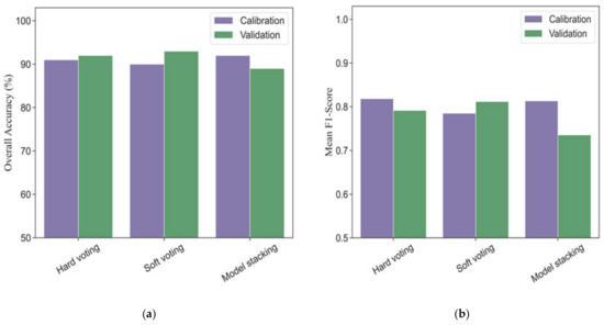
Figure 6.
The overall accuracies (a) and mean F1-scores (b) in different ensemble models for phenological detection in calibration and validation datasets.
Table 4.
The F1-scores in different ensemble models for detecting phenology in calibration and validation datasets.
In the validation dataset, the soft voting model (overall accuracy = 93% and mean F1-score = 0.81) outperformed the hard voting (overall accuracy = 92% and mean F1-score = 0.79) and model stacking (overall accuracy = 89% and mean F1-score = 0.74). As for individual phenology, the soft voting was slight better than the hard voting in terms of F1-scores, especially at the late stage of rice growth (Table 4). In addition, the model stacking strategy obtained worse accuracies than those in the hard voting and soft voting models for detecting the same phenological stage.
3.4. Single Best Model vs. Ensemble Models
Among five machine learning models, the GNB model with the best performance in terms of overall accuracy and mean F1-score in the validation dataset was selected to compare the reliability of phenological detection with ensemble models. Figure 7 presents the classification results obtained by GNB and ensemble models. It was observed that the vegetative stage was the most easily identified among the six phenological stages for all models. The heading stage in ensemble models was less confused with full heading stage than in the GNB model. Ripening phase is less confused with full heading stage as well. However, the capability for detecting full heading and maturity stage in the GNB model was slightly better than those in ensemble models.
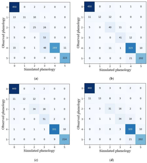
Figure 7.
The confusion matrixes of simulated and observed phenology achieved by GNB (a), hard voting (b), soft voting (c) and model stacking (d) using the validation dataset. Note: 0–5 represent vegetative, initial heading, heading, full heading, ripening and maturity stages, respectively.
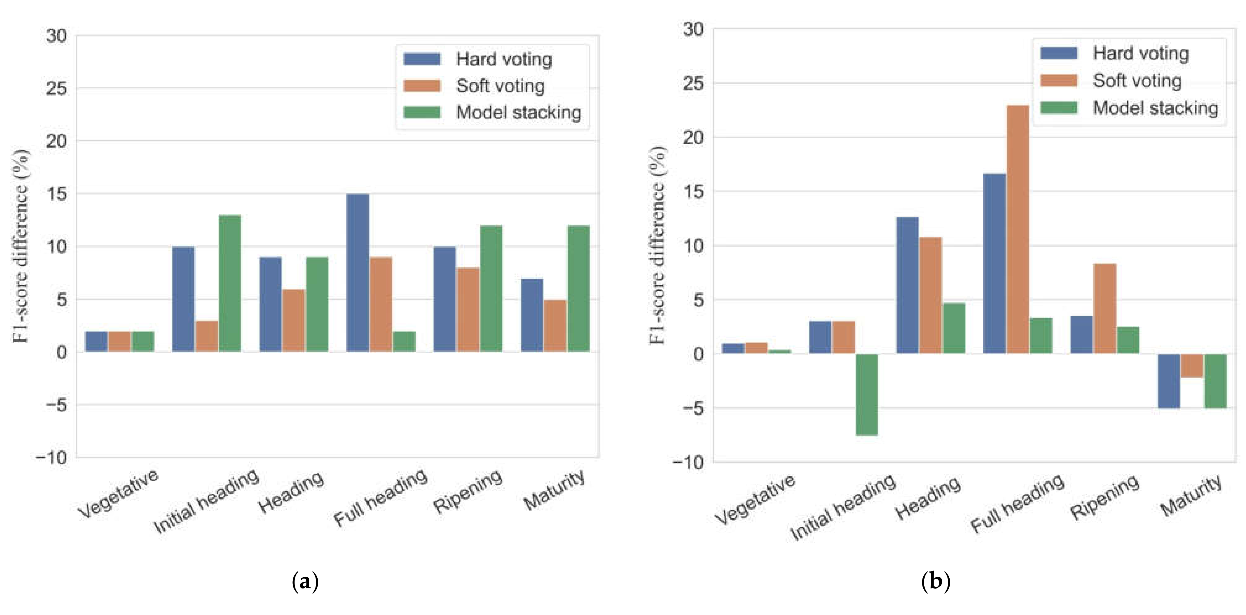
Figure 8 shows the differences in F1-scores between ensemble models and the GNB model. In the calibration dataset, all the ensemble models showed improvements of 2–15% for individual phenology detection in F1-scores relative to the performance of the GNB model. The ensemble models increased overall accuracies and mean F1-scores up to 6–9% and 5–7%, respectively, compared to the GNB model. In the validation dataset, all ensemble models had somewhat poor performance for maturity detection with the F1-scores reduced by 2.2–5.1%. As for overall accuracy and mean F1-score, the proposed ensemble models offered an improved accuracy in classification results with overall accuracy increased by 1–5%, and mean F1-scores increased by 0.2–7%.
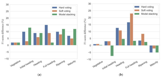
Figure 8.
Differences in F1-scores (%) between ensemble models and the single best classifier (GNB) in calibration (a) and validation (b) datasets.
In general, all ensemble models improved the classification accuracy to a certain extent, compared to the single best model (GNB). In addition, the highest classification accuracy was acquired by the soft voting algorithm, followed by the hard voting algorithm and finally by the model stacking.
4. Discussion
4.1. Feasibility of Ensemble Models for Phenology Detection
Many previous studies have successfully used the time-series VI data to capture vegetation phenology based on the function fitting or threshold method [6,18,61]. However, the accuracy of monitoring phenology is largely constrained by the temporal resolution of images [4]. In contrast, using machine learning algorithms or ensemble models to carry out phenology detection is another strategy without the limitation of temporal resolution, as long as there are enough training samples to identify each phenological stage. In this study, the performance of five machine learning algorithms and three ensemble models was compared to detect phenology in rice breeding. In terms of overall accuracy and F1-scores, all ensemble models were more accurate than the five individual classifiers in both calibration and validation datasets. Our results emphasized that the strategies to combine individual classifiers had the potential to improve phenology classification. This is consistent with literature that finds that ensemble models outperformed individual machine learning algorithms in many applications, such as mapping smallholder fields [37], predicting invasive plants [62] and forecasting corn yield [36].
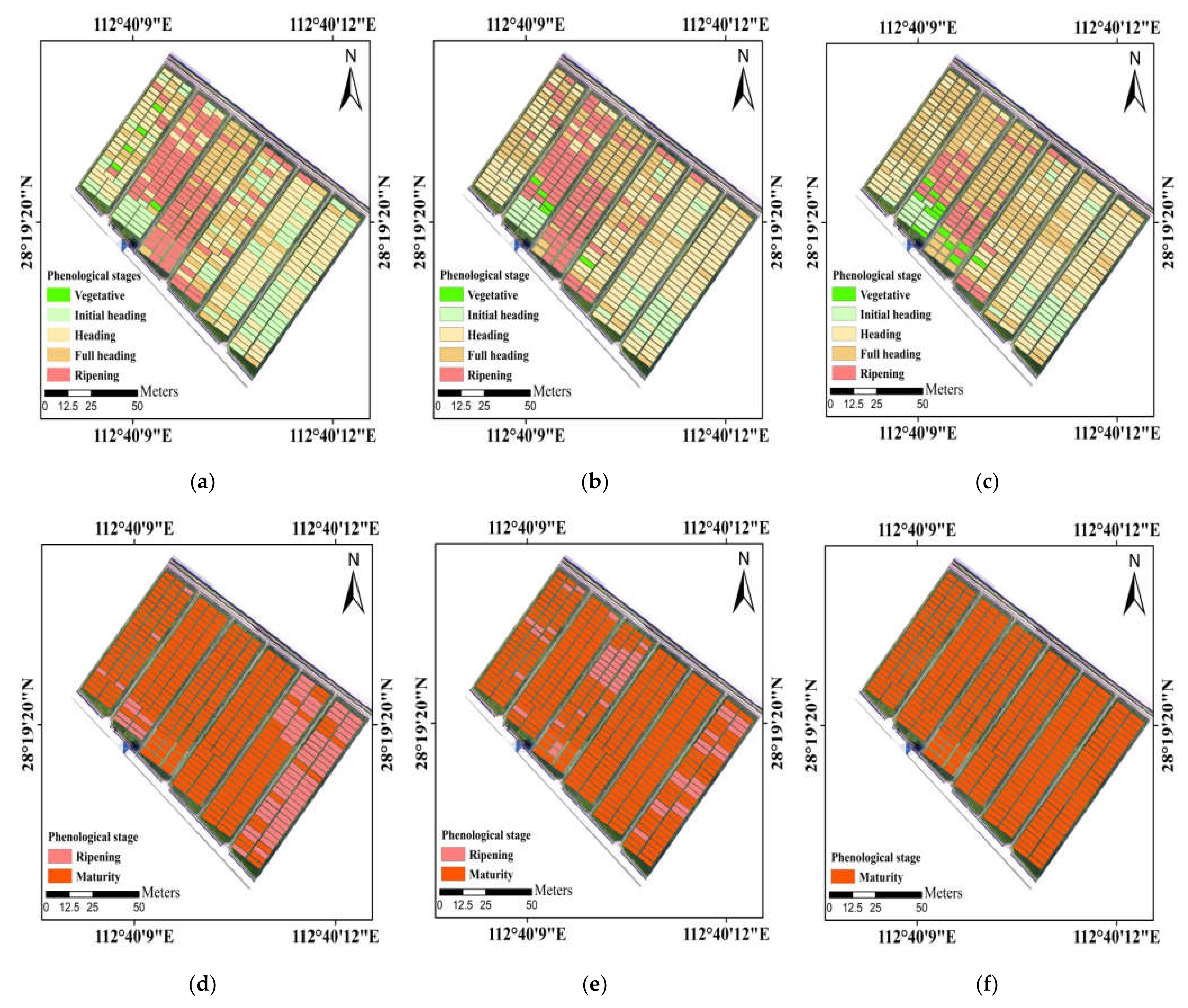
Among these ensemble models, the soft voting (weighted majority voting) performed best. In addition, maps produced by the soft voting appeared more homogeneous than the best individual classifier (GNB) in visual analysis (Figure 9). This is because the base classifiers which are more effective at detecting phenology would have more influence on the combined outputs. Polikar [59] also pointed out that the soft voting by weighting the decisions of qualified classifiers more heavily could improve the overall performance of classification more so than the hard voting (majority voting). The hard voting which obtained results based on the highest number of votes tended to be less accurate, most likely due to the strong correlations of predictions in base models. As for model stacking, GNB was only used as the meta-classifier, and the accuracy was slightly worse than the soft voting. The potential of using other machine learning or deep learning algorithms to fuse individual classifiers was necessarily investigated subsequently.

Figure 9.
Maps of principal phenological stages obtained from the visual observation (a,d), the predictions of soft voting (b,e) and GNB (c,f) in the study area. The UAV flights were carried out on (a–c) 11 September 2020 and (d–f) 1 November 2020.
Although the combination of individual classifiers can provide better phenological classification than a single classifier, the similarity of morphological characteristics in heading phase is still a challenge for ensemble models to exactly identify initial heading and full heading stages. In addition, the imbalanced training data could lead to poor classification [61]. Accordingly, the more representative samples in heading phase need to be further collected to improve the accuracy of ensemble models.
4.2. Combination of Feature Variables
In this study, three types (RGB-VIs, color space, textures) of feature variables were extracted from the UAV-RGB images to establish phenological prediction models. Although we did not compare the differences of performance of models based on RGB-VIs only, color space only and textures only, respectively; many previous studies have shown that fusion of multiple types of feature variables can improve the estimation accuracy of models [49,51,63,64]. Our research also confirms this point. The top five important variables come from different types of variables in the three ensemble models (Table 5). In addition, other auxiliary data derived from UAV-RGB imagery, such as 3D point cloud and canopy coverage of each plot, should be added as they may result in higher estimation accuracy. This is something which needs to be investigated in future with procedures to estimate rice phenological stages using more input features. Furthermore, the proposed ensemble models could be used to obtain insight into critical factors which determine the variability of phenology in rice breeding for breeders and agronomists.
Table 5.
Feature ranking in ensemble models based on variable importance.
4.3. Potential of UAV-Based Imagery in Rice Breeding Trails
In recent years, the rapid development of UAVs and sensors along with improved computer capacities for data analyses has enabled a range of possibilities to estimate plant traits in high throughput filed phenotyping [65]. Compared to fixed-position cameras and satellites, the UAV platforms had a better trade-off between revisit time, spatial resolution, price and data accuracy [66]. In particular, the phenotyping occurs at a relatively small plot scale in breeding trails. The flight altitudes of UAVs can be flexibly set by the requirements of experiments to capture ultra-high resolution images. The high spatial resolution of field phenotyping is a prerequisite to distinguish the changes of morphology in rice breeding which failed to be detected by satellites. In this study, the imagery with an ultra-high resolution of 1.36 cm was used to calculated feature variables. This resolution can track the temporal pattern of canopy color changes during crop growth season. In future, integrating the phenotypic information derived from UAVs into crop models to help decision making in agriculture management could bring large benefits in optimizing resource utilization to improve breeding efficiency.
5. Conclusions
In this study, three types of ensemble model were proposed to identify principal phenological stages in rice breeding trials using UAV-based RGB imagery. In contrast to the curve fitting or shape model fitting methods based on time-series VI data, the ensemble models could detect phenology from the mono-temporal UAV imagery. Results showed that all the ensemble models showed improvements of 1–5% in overall accuracy and 0.2–7% in mean F1-scores compared to the best individual classifier (GNB) for phenology detection in the validation dataset. Among the ensemble models, the soft voting had the best performance, followed by the hard voting and finally by the model stacking. The ensemble techniques presented in this study are promising and valuable to improve the accuracy of phenology detection in rice breeding, thus promoting the breeding processes.
Author Contributions
Conceptualization, H.G.; methodology, H.G.; investigation, C.D., H.G., F.M., Z.L. and Z.T.; resources, C.D.; data curation, H.G.; writing—original draft preparation, H.G.; writing—review and editing, C.D.; visualization, H.G.; supervision, C.D. All authors have read and agreed to the published version of the manuscript.
Funding
This study was supported by the Key Research and Development Program of Shandong Province (2019JZZY010713) and National Key Research and Development Program of China (No. 2018YFE0107000).
Institutional Review Board Statement
Not applicable.
Informed Consent Statement
Not applicable.
Data Availability Statement
Data sharing not applicable.
Acknowledgments
Thanks to Jingyou Guo and Youdong Hu for providing the details of the experimental design in this study.
Conflicts of Interest
The authors declare no conflict of interest.
Appendix A
Table A1.
Description of tuning parameters in the five machine learning algorithms with 10-fold cross validation.
Table A1.
Description of tuning parameters in the five machine learning algorithms with 10-fold cross validation.
| Model | Parameters | Range | The Optimal Value |
|---|---|---|---|
| RF | max_depth | 10–100 (interval: 10) | 50 |
| n_estimators | 3–15 (interval: 1) | 6 | |
| KNN | n_neighbors | 1–5 | 5 |
| GNB | -- | -- | default |
| SVM | C | 1–11 | 2 |
| kernel | ‘linear’ and ‘rbf’ | ‘linear’ | |
| LR | C | 1-11 | 4 |
| penalty | ‘L1′ and ‘L2′ | ‘L1′ | |
| solver | ‘liblinear’, ‘lbfgs’, ‘newton-cg’,’sag’ | ‘liblinear’ |
References
- Ma, Y.; Jiang, Q.; Wu, X.; Zhu, R.; Gong, Y.; Peng, Y.; Duan, B.; Fang, S. Monitoring hybrid rice phenology at initial heading stage based on low-altitude remote sensing data. Remote Sens. 2021, 13, 86. [Google Scholar] [CrossRef]
- Stoeckli, R.; Rutishauser, T.; Dragoni, D.; O’Keefe, J.; Thornton, P.E.; Jolly, M.; Lu, L.; Denning, A.S. Remote sensing data assimilation for a prognostic phenology model. J. Geophys. Res. Biogeosci. 2008, 113, G04021. [Google Scholar] [CrossRef]
- Mongiano, G.; Titone, P.; Pagnoncelli, S.; Sacco, D.; Tamborini, L.; Pilu, R.; Bregaglio, S. Phenotypic variability in Italian rice germplasm. Eur. J. Agron. 2020, 120, 126131. [Google Scholar] [CrossRef]
- Yang, Q.; Shi, L.; Han, J.; Yu, J.; Huang, K. A near real-time deep learning approach for detecting rice phenology based on UAV images. Agric. For. Meteorol. 2020, 287, 107938. [Google Scholar] [CrossRef]
- Haghshenas, A.; Emam, Y. Image-based tracking of ripening in wheat cultivar mixtures: A quantifying approach parallel to the conventional phenology. Comput. Electron. Agric. 2019, 156, 318–333. [Google Scholar] [CrossRef]
- Pan, Z.; Huang, J.; Zhou, Q.; Wang, L.; Cheng, Y.; Zhang, H.; Blackburn, G.A.; Yan, J.; Liu, J. Mapping crop phenology using NDVI time-series derived from HJ-1 A/B data. Int. J. Appl. Earth Obs. Geoinf. 2015, 34, 188–197. [Google Scholar] [CrossRef] [Green Version]
- Sakamoto, T.; Wardlow, B.D.; Gitelson, A.A.; Verma, S.B.; Suyker, A.E.; Arkebauer, T.J. A two-step filtering approach for detecting maize and soybean phenology with time-series MODIS data. Remote Sens. Environ. 2010, 114, 2146–2159. [Google Scholar] [CrossRef]
- Sakamoto, T.; Yokozawa, M.; Toritani, H.; Shibayama, M.; Ishitsuka, N.; Ohno, H. A crop phenology detection method using time-series MODIS data. Remote Sens. Environ. 2005, 96, 366–374. [Google Scholar] [CrossRef]
- Thompson, D.R.; Wehmanen, O.A. Using Landsat digital data to detect moisture stress. Photogramm. Eng. Remote Sens. 1979, 45, 201–207. [Google Scholar]
- Qiu, B.; Luo, Y.; Tang, Z.; Chen, C.; Lu, D.; Huang, H.; Chen, Y.; Chen, N.; Xu, W. Winter wheat mapping combining variations before and after estimated heading dates. ISPRS J. Photogramm. Remote Sens. 2017, 123, 35–46. [Google Scholar] [CrossRef]
- Wu, X.; Yang, W.; Wang, C.; Shen, Y.; Kondoh, A. Interactions among the phenological events of winter wheat in the north China plain-based on field data and improved MODIS estimation. Remote Sens. 2019, 11, 2976. [Google Scholar] [CrossRef] [Green Version]
- Singha, M.; Wu, B.; Zhang, M. An object-based paddy rice classification using multi-spectral data and crop phenology in Assam, northeast India. Remote Sens. 2016, 8, 479. [Google Scholar] [CrossRef] [Green Version]
- Onojeghuo, A.O.; Blackburn, G.A.; Wang, Q.; Atkinson, P.M.; Kindred, D.; Miao, Y. Rice crop phenology mapping at high spatial and temporal resolution using downscaled MODIS time-series. GIsci. Remote Sens. 2018, 55, 659–677. [Google Scholar] [CrossRef] [Green Version]
- Singha, M.; Sarmah, S. Incorporating crop phenological trajectory and texture for paddy rice detection with time series MODIS, HJ-1A and ALOS PALSAR imagery. Eur. J. Remote Sens. 2019, 52, 73–87. [Google Scholar] [CrossRef] [Green Version]
- Kibret, K.S.; Marohn, C.; Cadisch, G. Use of MODIS EVI to map crop phenology, identify cropping systems, detect land use change and drought risk in Ethiopia—An application of Google Earth Engine. Eur. J. Remote Sens. 2020, 53, 176–191. [Google Scholar] [CrossRef]
- Ren, J.; Campbell, J.B.; Shao, Y. Estimation of SOS and EOS for midwestern US corn and soybean crops. Remote Sens. 2017, 9, 722. [Google Scholar] [CrossRef] [Green Version]
- Wardlow, B.D.; Kastens, J.H.; Egbert, S.L. Using USDA crop progress data for the evaluation of greenup onset date calculated from MODIS 250-meter data. Photogramm. Eng. Remote Sens. 2006, 72, 1225–1234. [Google Scholar] [CrossRef] [Green Version]
- Vrieling, A.; Meroni, M.; Darvishzadeh, R.; Skidmore, A.K.; Wang, T.; Zurita-Milla, R.; Oosterbeek, K.; O’Connor, B.; Paganini, M. Vegetation phenology from Sentinel-2 and field cameras for a Dutch barrier island. Remote Sens. Environ. 2018, 215, 517–529. [Google Scholar] [CrossRef]
- Zhou, M.; Ma, X.; Wang, K.; Cheng, T.; Tian, Y.; Wang, J.; Zhu, Y.; Hu, Y.; Niu, Q.; Gui, L.; et al. Detection of phenology using an improved shape model on time-series vegetation index in wheat. Comput. Electron. Agric. 2020, 173, 105398. [Google Scholar] [CrossRef]
- Wang, H.; Magagi, R.; Goita, K.; Trudel, M.; McNairn, H.; Powers, J. Crop phenology retrieval via polarimetric SAR decomposition and Random Forest algorithm. Remote Sens. Environ. 2019, 231, 111234. [Google Scholar] [CrossRef]
- Fikriyah, V.N.; Darvishzadeh, R.; Laborte, A.; Khan, N.I.; Nelson, A. Discriminating transplanted and direct seeded rice using Sentinel-1 intensity data. Int. J. Appl. Earth Obs. Geoinf. 2019, 76, 143–153. [Google Scholar] [CrossRef] [Green Version]
- He, Z.; Li, S.; Wang, Y.; Dai, L.; Lin, S. Monitoring rice phenology based on backscattering characteristics of multi-temporal RADARSAT-2 datasets. Remote Sens. 2018, 10, 340. [Google Scholar] [CrossRef] [Green Version]
- Duan, T.; Chapman, S.C.; Guo, Y.; Zheng, B. Dynamic monitoring of NDVI in wheat agronomy and breeding trials using an unmanned aerial vehicle. Field Crop. Res. 2017, 210, 71–80. [Google Scholar] [CrossRef]
- Zeng, L.; Wardlow, B.D.; Xiang, D.; Hu, S.; Li, D. A review of vegetation phenological metrics extraction using time-series, multispectral satellite data. Remote Sens. Environ. 2020, 237, 111511. [Google Scholar] [CrossRef]
- Park, J.Y.; Muller-Landau, H.C.; Lichstein, J.W.; Rifai, S.W.; Dandois, J.P.; Bohlman, S.A. Quantifying leaf phenology of individual trees and species in a tropical forest using Unmanned Aerial Vehicle (UAV) images. Remote Sens. 2019, 11, 1534. [Google Scholar] [CrossRef] [Green Version]
- Burkart, A.; Hecht, V.L.; Kraska, T.; Rascher, U. Phenological analysis of unmanned aerial vehicle based time series of barley imagery with high temporal resolution. Precis. Agric. 2017, 19, 134–146. [Google Scholar] [CrossRef]
- Chen, J.; Jonsson, P.; Tamura, M.; Gu, Z.H.; Matsushita, B.; Eklundh, L. A simple method for reconstructing a high-quality NDVI time-series data set based on the Savitzky-Golay filter. Remote Sens. Environ. 2004, 91, 332–344. [Google Scholar] [CrossRef]
- Jonsson, P.; Eklundh, L. Seasonality extraction by function fitting to time-series of satellite sensor data. IEEE Trans. Geosci. Remote Sens. 2002, 40, 1824–1832. [Google Scholar] [CrossRef]
- Zhang, X.Y.; Friedl, M.A.; Schaaf, C.B.; Strahler, A.H.; Hodges, J.C.F.; Gao, F.; Reed, B.C.; Huete, A. Monitoring vegetation phenology using MODIS. Remote Sens. Environ. 2003, 84, 471–475. [Google Scholar] [CrossRef]
- Cao, J.; Zhang, Z.; Tao, F.; Zhang, L.; Luo, Y.; Zhang, J.; Han, J.; Xie, J. Integrating multi-source data for rice yield prediction across China using machine learning and deep learning approaches. Agric. For. Meteorol. 2021, 297, 108275. [Google Scholar] [CrossRef]
- Carbonneau, P.E.; Dugdale, S.J.; Breckon, T.P.; Dietrich, J.T.; Fonstad, M.A.; Miyamoto, H.; Woodget, A.S. Adopting deep learning methods for airborne RGB fluvial scene classification. Remote Sens. Environ. 2020, 251, 112107. [Google Scholar] [CrossRef]
- Li, J.; Wu, Z.; Hu, Z.; Li, Z.; Wang, Y.; Molinier, M. Deep learning based thin cloud removal fusing vegetation red edge and short wave infrared spectral information for Sentinel-2A imagery. Remote Sens. 2021, 13, 157. [Google Scholar] [CrossRef]
- Sandhu, K.S.; Lozada, D.N.; Zhang, Z.; Pumphrey, M.O.; Carter, A.H. Deep Learning for Predicting Complex Traits in Spring Wheat Breeding Program. Front. Plant Sci. 2021, 11, 613325. [Google Scholar] [CrossRef]
- Hieu, P.; Olafsson, S. On Cesaro Averages for Weighted Trees in the Random Forest. J. Classif. 2020, 37, 223–236. [Google Scholar] [CrossRef]
- Hieu, P.; Olafsson, S. Bagged ensembles with tunable parameters. Comput. Intell. 2019, 35, 184–203. [Google Scholar] [CrossRef]
- Shahhosseini, M.; Hu, G.; Archontoulis, S.V. Forecasting Corn Yield With Machine Learning Ensembles. Front. Plant Sci. 2020, 11, 1120. [Google Scholar] [CrossRef]
- Masiza, W.; Chirima, J.G.; Hamandawana, H.; Pillay, R. Enhanced mapping of a smallholder crop farming landscape through image fusion and model stacking. Int. J. Remote Sens. 2020, 41, 8739–8756. [Google Scholar] [CrossRef]
- Fageria, N.K. Yield physiology of rice. J. Plant Nutr. 2007, 30, 843–879. [Google Scholar] [CrossRef]
- Zheng, H.; Cheng, T.; Li, D.; Zhou, X.; Yao, X.; Tian, Y.; Cao, W.; Zhu, Y. Evaluation of RGB, color-infrared and multispectral images acquired from unmanned aerial systems for the estimation of nitrogen accumulation in rice. Remote Sens. 2018, 10, 824. [Google Scholar] [CrossRef] [Green Version]
- Lucieer, A.; Turner, D.; King, D.H.; Robinson, S.A. Using an Unmanned Aerial Vehicle (UAV) to capture micro-topography of Antarctic moss beds. Int. J. Appl. Earth Obs. Geoinf. 2014, 27, 53–62. [Google Scholar] [CrossRef] [Green Version]
- Yu, N.; Li, L.; Schmitz, N.; Tiaz, L.F.; Greenberg, J.A.; Diers, B.W. Development of methods to improve soybean yield estimation and predict plant maturity with an unmanned aerial vehicle based platform. Remote Sens. Environ. 2016, 187, 91–101. [Google Scholar] [CrossRef]
- Liu, K.; Li, Y.; Han, T.; Yu, X.; Ye, H.; Hu, H.; Hu, Z. Evaluation of grain yield based on digital images of rice canopy. Plant Methods 2019, 15, 28. [Google Scholar] [CrossRef]
- Woebbecke, D.M.; Meyer, G.E.; Vonbargen, K.; Mortensen, D.A. Color indices for weed identification under various soil, residue, and lighting conditions. Trans. Am. Soc. Agric. Biol. Eng. 1995, 38, 259–269. [Google Scholar] [CrossRef]
- Meyer, G.E.; Neto, J.C. Verification of color vegetation indices for automated crop imaging applications. Comput. Electron. Agric. 2008, 63, 282–293. [Google Scholar] [CrossRef]
- Li, Y.; Chen, D.; Walker, C.N.; Angus, J.F. Estimating the nitrogen status of crops using a digital camera. Field Crop. Res. 2010, 118, 221–227. [Google Scholar] [CrossRef]
- Fu, Y.; Yang, G.; Li, Z.; Song, X.; Li, Z.; Xu, X.; Wang, P.; Zhao, C. Winter wheat nitrogen status estimation using UAV-based RGB imagery and gaussian processes regression. Remote Sens. 2020, 12, 3778. [Google Scholar] [CrossRef]
- Haralick, R.M.; Shanmugam, K.; Dinstein, I. Textural features for image classification. IEEE Trans. Syst. Man Cybern. 1973, 6, 610–621. [Google Scholar] [CrossRef] [Green Version]
- Hall-Beyer, M. Practical guidelines for choosing GLCM textures to use in landscape classification tasks over a range of moderate spatial scales. Int. J. Remote Sens. 2017, 38, 1312–1338. [Google Scholar] [CrossRef]
- Li, S.; Yuan, F.; Ata-Ui-Karim, S.T.; Zheng, H.; Cheng, T.; Liu, X.; Tian, Y.; Zhu, Y.; Cao, W.; Cao, Q. Combining color indices and textures of UAV-based digital imagery for rice LAI estimation. Remote Sens. 2019, 11, 1763. [Google Scholar] [CrossRef] [Green Version]
- Yue, J.; Yang, G.; Tian, Q.; Feng, H.; Xu, K.; Zhou, C. Estimate of winter-wheat above-ground biomass based on UAV ultrahigh-ground-resolution image textures and vegetation indices. ISPRS J. Photogramm. Remote Sens. 2019, 150, 226–244. [Google Scholar] [CrossRef]
- Zheng, H.; Ma, J.; Zhou, M.; Li, D.; Yao, X.; Cao, W.; Zhu, Y.; Cheng, T. Enhancing the nitrogen signals of rice canopies across critical growth stages through the integration of textural and spectral information from Unmanned Aerial Vehicle (UAV) multispectral imagery. Remote Sens. 2020, 12, 957. [Google Scholar] [CrossRef] [Green Version]
- Wood, E.M.; Pidgeon, A.M.; Radeloff, V.C.; Keuler, N.S. Image texture as a remotely sensed measure of vegetation structure. Remote Sens. Environ. 2012, 121, 516–526. [Google Scholar] [CrossRef]
- Breiman, L. Random Forests. Mach. Learn. 2001, 45, 5–32. [Google Scholar] [CrossRef] [Green Version]
- Aguilar, R.; Zurita-Milla, R.; Izquierdo-Verdiguier, E.; de By, R.A. A cloud-based multi-temporal ensemble classifier to map smallholder farming systems. Remote Sens. 2018, 10, 729. [Google Scholar] [CrossRef] [Green Version]
- Wang, S.C.; Gao, R.; Wang, L.M. Bayesian network classifiers based on Gaussian kernel density. Expert Syst. Appl. 2016, 51, 207–217. [Google Scholar] [CrossRef]
- Buhlmann, P.; Yu, B. Additive logistic regression: A statistical view of boosting—Discussion. Ann. Stat. 2000, 28, 377–386. [Google Scholar] [CrossRef]
- Pena, J.M.; Gutierrez, P.A.; Hervas-Martinez, C.; Six, J.; Plant, R.E.; Lopez-Granados, F. Object-based image classification of summer crops with machine learning methods. Remote Sens. 2014, 6, 5019–5041. [Google Scholar] [CrossRef] [Green Version]
- Gutierrez, P.A.; Lopez-Granados, F.; Pena-Barragan, J.M.; Jurado-Exposito, M.; Hervas-Martinez, C. Logistic regression product-unit neural networks for mapping Ridolfia segetum infestations in sunflower crop using multitemporal remote sensed data. Comput. Electron. Agric. 2008, 64, 293–306. [Google Scholar] [CrossRef]
- Polikar, R. Essemble based systems in decision making. IEEE Circuits Syst. Mag. 2006, 6, 21–45. [Google Scholar] [CrossRef]
- Wozniak, M.; Grana, M.; Corchado, E. A survey of multiple classifier systems as hybrid systems. Inf. Fusion 2014, 16, 3–17. [Google Scholar] [CrossRef] [Green Version]
- Zheng, H.; Cheng, T.; Yao, X.; Deng, X.; Tian, Y.; Cao, W.; Zhu, Y. Detection of rice phenology through time series analysis of ground-based spectral index data. Field Crop. Res. 2016, 198, 131–139. [Google Scholar] [CrossRef]
- Fang, Y.; Zhang, X.; Wei, H.; Wang, D.; Chen, R.; Wang, L.; Gu, W. Predicting the invasive trend of exotic plants in China based on the ensemble model under climate change: A case for three invasive plants of Asteraceae. Sci. Total Environ. 2021, 756, 143841. [Google Scholar] [CrossRef]
- Lin, F.; Zhang, D.; Huang, Y.; Wang, X.; Chen, X. Detection of corn and weed species by the combination of spectral, shape and textural features. Sustainability 2017, 9, 1335. [Google Scholar] [CrossRef] [Green Version]
- Liu, Y.; Liu, S.; Li, J.; Guo, X.; Wang, S.; Lu, J. Estimating biomass of winter oilseed rape using vegetation indices and texture metrics derived from UAV multispectral images. Comput. Electron. Agric. 2019, 166, 105026. [Google Scholar] [CrossRef]
- Volpato, L.; Pinto, F.; Gonzalez-Perez, L.; Thompson, I.G.; Borem, A.; Reynolds, M.; Gerard, B.; Molero, G.; Rodrigues, F.A., Jr. High throughput field phenotyping for plant height using uav-based rgb imagery in wheat breeding lines: Feasibility and validation. Front. Plant Sci. 2021, 12, 591587. [Google Scholar] [CrossRef]
- Zhao, C.; Zhang, Y.; Du, J.; Guo, X.; Wen, W.; Gu, S.; Wang, J.; Fan, J. Crop phenomics: Current status and perspectives. Front. Plant Sci. 2019, 10, 714. [Google Scholar] [CrossRef] [Green Version]


Publisher’s Note: MDPI stays neutral with regard to jurisdictional claims in published maps and institutional affiliations. |
© 2021 by the authors. Licensee MDPI, Basel, Switzerland. This article is an open access article distributed under the terms and conditions of the Creative Commons Attribution (CC BY) license (https://creativecommons.org/licenses/by/4.0/).