
Fine-Tuning Heat Stress Algorithms to Optimise Global Predictions of Mass Coral Bleaching

 , , and
Abstract
:
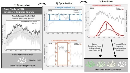
1. Introduction
2. Materials and Methods
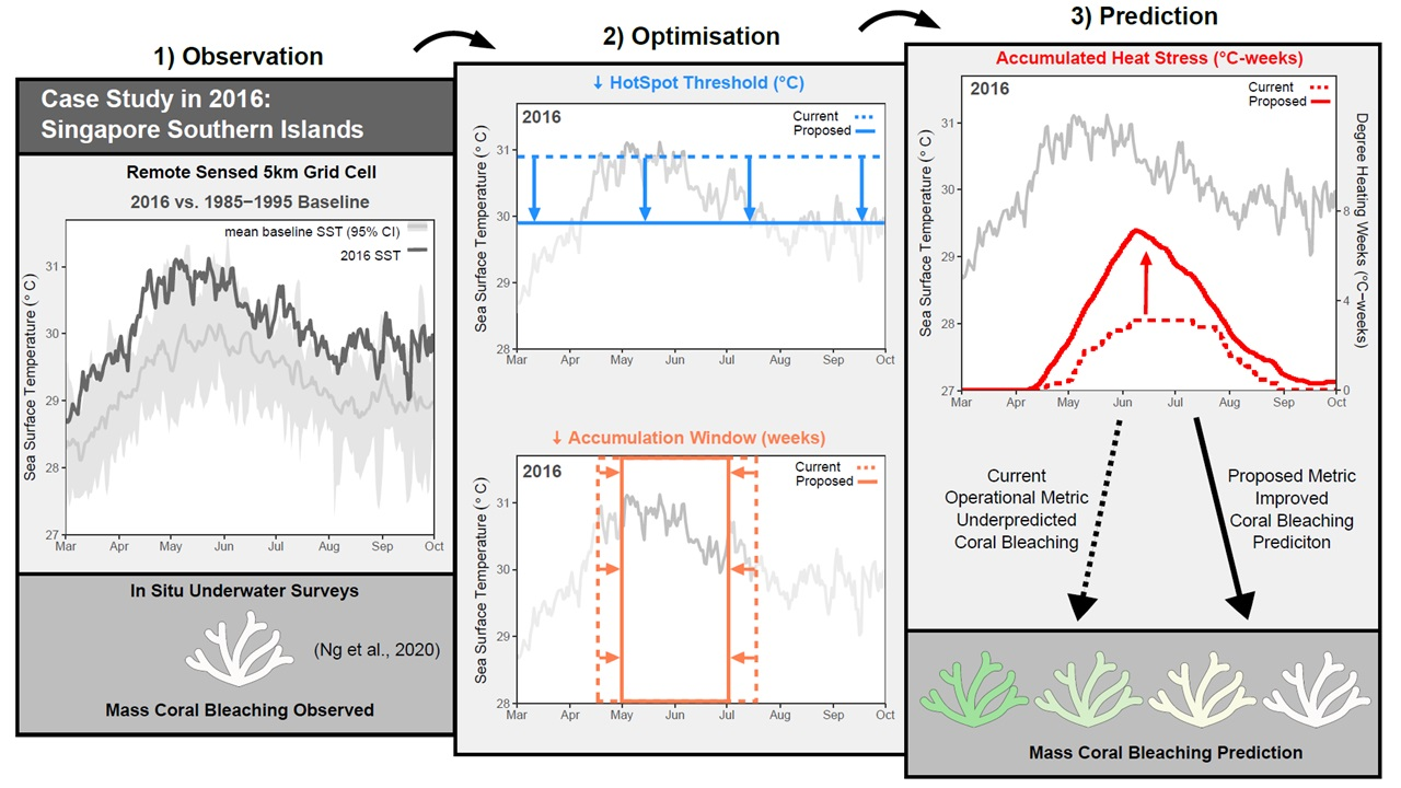
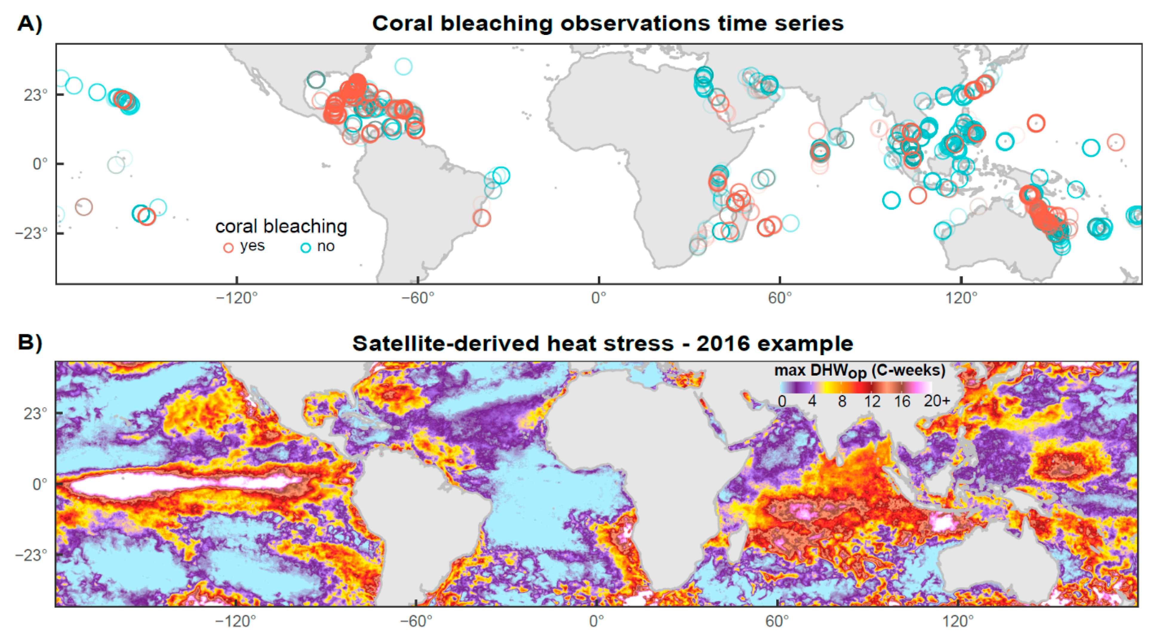
2.1. Coral Bleaching Data
2.2. Temperature Data
2.3. Statistical Approach
- For each DHW metric, the association with coral bleaching was tested using a spatiotemporal generalised linear model (GLM) with a Bernoulli error structure using INLA.
- Sensitivity–specificity analysis was performed on this GLM to optimise predictions, tally model successes and failures and provide metrics for model comparisons.
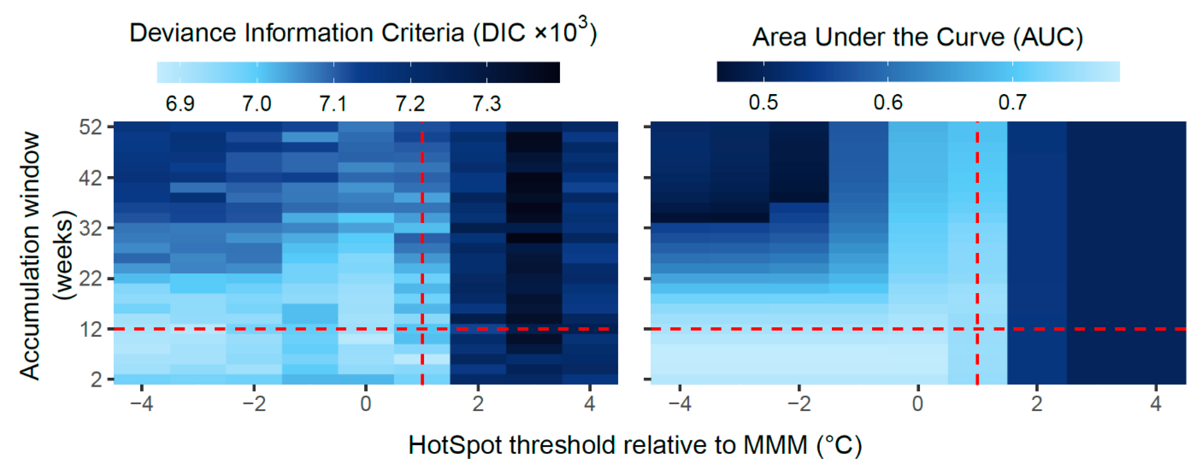
- The first two steps were repeated for all DHWtest metrics and DHWop, resulting in 235 separate GLMs and sensitivity–specificity analyses, each run in parallel on separate Intel Xeon E5-2699 processors via the high-performance computing cluster “The Rocket”.
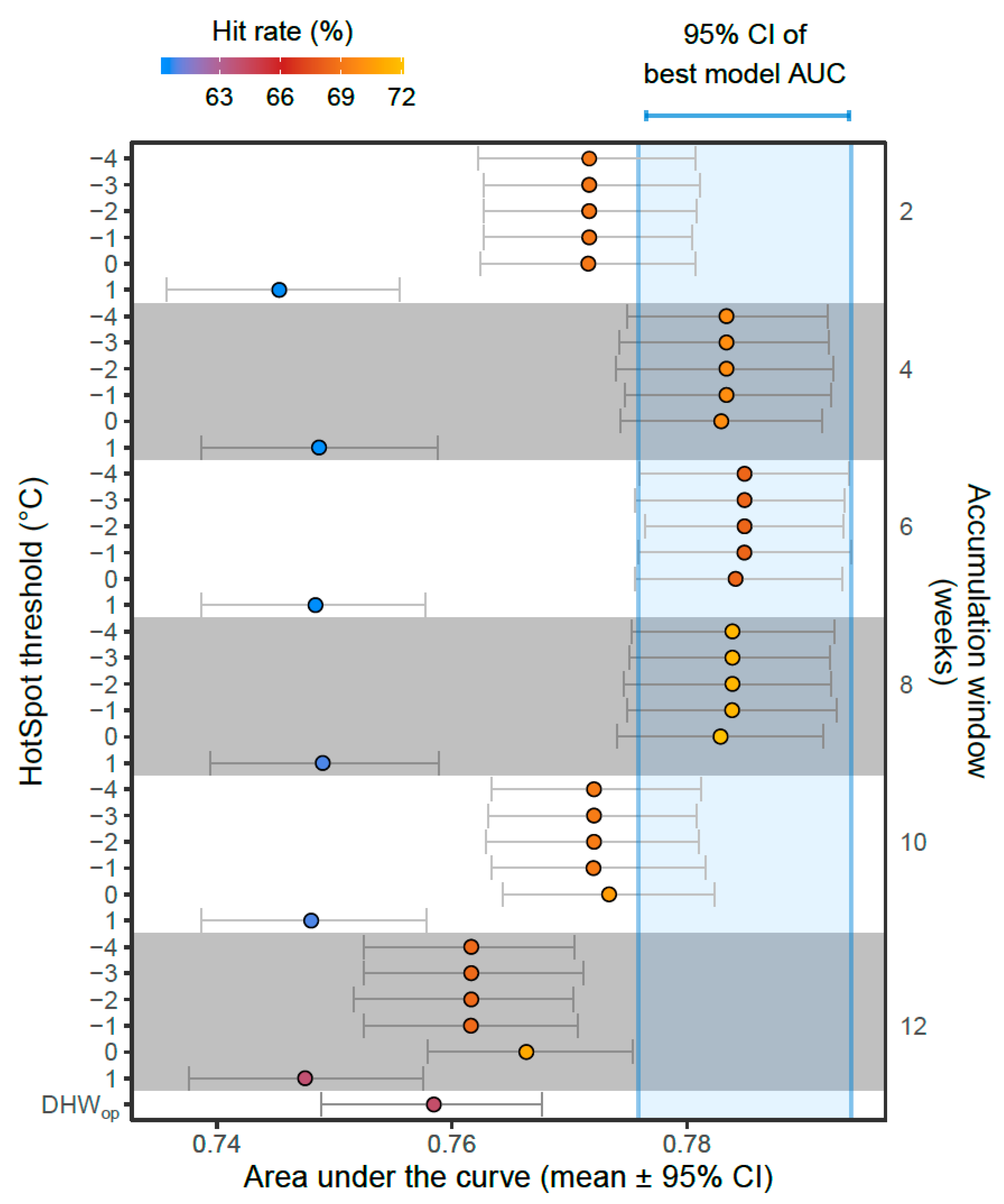
- Model comparisons were used to determine the best-performing models and hence the optimal HotSpot threshold and accumulation window for predicting coral bleaching globally using DHWs.
2.4. Model Formulation
2.5. Model Validation
2.6. Sensitivity–Specificity Analysis
2.7. Model Comparisons
3. Results
3.1. Model Comparisons
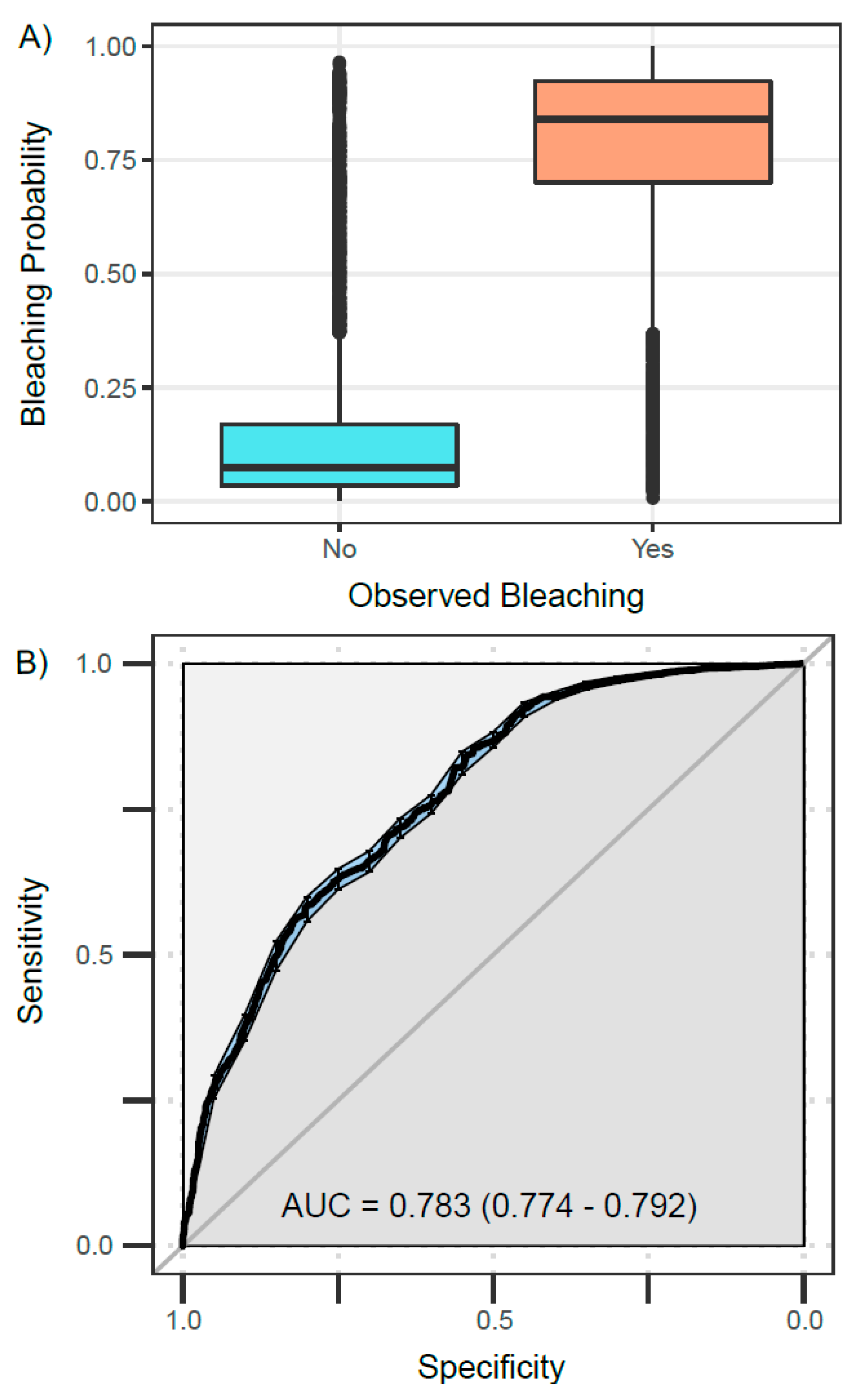
3.2. Best Model—Validation
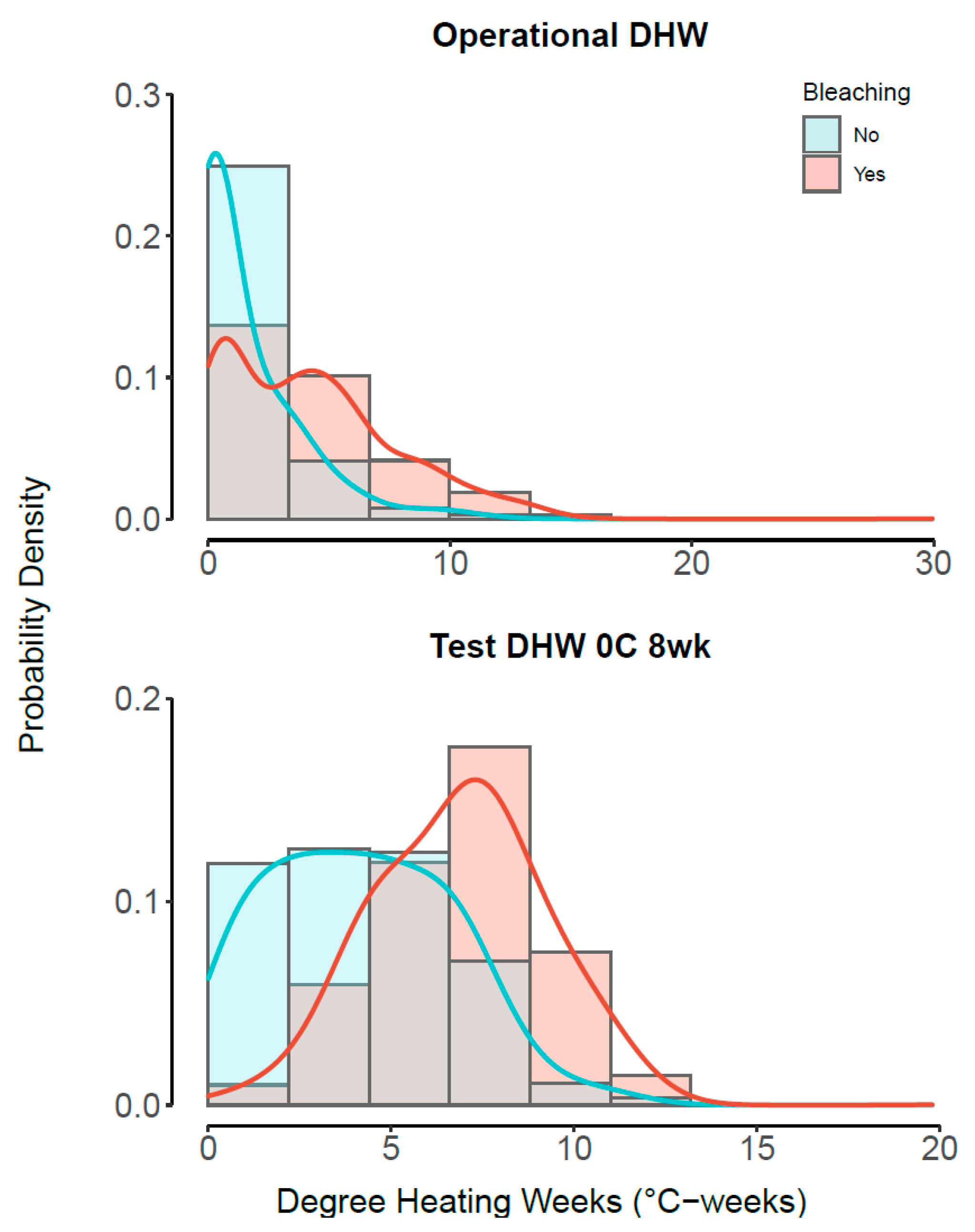
3.3. Best Model—Understanding Heat Stress
4. Discussion
4.1. Complexities of Coral Bleaching
4.2. Global and Regional Scales
4.3. Alternate Heat Stress Algorithm Applications
5. Conclusions
Supplementary Materials
Author Contributions
Funding
Institutional Review Board Statement
Informed Consent Statement
Data Availability Statement
Acknowledgments
Conflicts of Interest
References
- Oliver, E.C.J.; Donat, M.G.; Burrows, M.T.; Moore, P.; Smale, D.A.; Alexander, L.V.; Benthuysen, J.; Feng, M.; Gupta, A.S.; Hobday, A.J.; et al. Longer and more frequent marine heatwaves over the past century. Nat. Commun. 2018, 9, 1324. [Google Scholar] [CrossRef] [PubMed]
- Holbrook, N.J.; Scannell, H.A.; Gupta, A.S.; Benthuysen, J.A.; Feng, M.; Oliver, E.C.J.; Alexander, L.V.; Burrows, M.T.; Donat, M.G.; Hobday, A.J.; et al. A global assessment of marine heatwaves and their drivers. Nat. Commun. 2019, 10, 1–13. [Google Scholar] [CrossRef]
- Jiménez-Quiroz, M.D.C.; Cervantes-Duarte, R.; Funes-Rodríguez, R.; Barón-Campis, S.A.; García-Romero, F.D.J.; Hernández-Trujillo, S.; Hernández-Becerril, D.U.; González-Armas, R.; Martell-Dubois, R.; Cerdeira-Estrada, S.; et al. Impact of “The Blob” and “El Niño” in the SW Baja California Peninsula: Plankton and Environmental Variability of Bahia Magdalena. Front. Mar. Sci. 2019, 6, 1–23. [Google Scholar] [CrossRef] [Green Version]
- Evans, R.; Lea, M.-A.; Hindell, M.; Swadling, K. Significant shifts in coastal zooplankton populations through the 2015/16 Tasman Sea marine heatwave. Estuar. Coast. Shelf Sci. 2020, 235, 106538. [Google Scholar] [CrossRef]
- Işkın, U.; Filiz, N.; Cao, Y.; Neif, É.M.; Öğlü, B.; Lauridsen, T.L.; Davidson, T.A.; Søndergaard, M.; Tavşanoğlu, Ü.N.; Beklioğlu, M.; et al. Impact of Nutrients, Temperatures, and a Heat Wave on Zooplankton Community Structure: An Experimental Approach. Water 2020, 12, 3416. [Google Scholar] [CrossRef]
- Piatt, J.F.; Parrish, J.K.; Renner, H.M.; Schoen, S.K.; Jones, T.T.; Arimitsu, M.L.; Kuletz, K.J.; Bodenstein, B.; García-Reyes, M.; Duerr, R.S.; et al. Extreme mortality and reproductive failure of common murres resulting from the northeast Pacific marine heatwave of 2014–2016. PLoS ONE 2020, 15, e0226087. [Google Scholar] [CrossRef] [Green Version]
- Jones, T.; Parrish, J.K.; Peterson, W.T.; Bjorkstedt, E.P.; Bond, N.A.; Ballance, L.T.; Bowes, V.; Hipfner, J.M.; Burgess, H.K.; Dolliver, J.E.; et al. Massive Mortality of a Planktivorous Seabird in Response to a Marine Heatwave. Geophys. Res. Lett. 2018, 45, 3193–3202. [Google Scholar] [CrossRef]
- Cavole, L.; Oceanography, S.I.O.; Demko, A.; Diner, R.; Giddings, A.; Koester, I.; Pagniello, C.; Paulsen, M.-L.; Ramirez-Valdez, A.; Schwenck, S.; et al. Biological Impacts of the 2013–2015 Warm-Water Anomaly in the Northeast Pacific: Winners, Losers, and the Future. Oceanography 2016, 29, 273–285. [Google Scholar] [CrossRef] [Green Version]
- Hughes, T.P.; Anderson, K.D.; Connolly, S.R.; Heron, S.F.; Kerry, J.T.; Lough, J.M.; Baird, A.H.; Baum, J.K.; Berumen, M.L.; Bridge, T.C.; et al. Spatial and temporal patterns of mass bleaching of corals in the Anthropocene. Science 2018, 359, 80–83. [Google Scholar] [CrossRef] [Green Version]
- Costanza, R.; De Groot, R.; Sutton, P.; van der Ploeg, S.; Anderson, S.J.; Kubiszewski, I.; Farber, S.; Turner, R.K. Changes in the global value of ecosystem services. Glob. Environ. Chang. 2014, 26, 152–158. [Google Scholar] [CrossRef]
- Ferrario, F.; Beck, M.W.; Storlazzi, C.D.; Micheli, F.; Shepard, C.C.; Airoldi, L. The effectiveness of coral reefs for coastal hazard risk reduction and adaptation. Nat. Commun. 2014, 5, 3794. [Google Scholar] [CrossRef]
- Hughes, T.P.; Kerry, J.T.; Álvarez-Noriega, M.; Álvarez-Romero, J.G.; Anderson, K.D.; Baird, A.H.; Babcock, R.C.; Beger, M.; Bellwood, D.R.; Berkelmans, R.; et al. Global warming and recurrent mass bleaching of corals. Nature 2017, 543, 373–377. [Google Scholar] [CrossRef] [PubMed]
- Brown, B.E. Coral bleaching: Causes and consequences. Coral Reefs 1997, 16, S129–S138. [Google Scholar] [CrossRef]
- Edmunds, P.J. The effect of sub-lethal increases in temperature on the growth and population trajectories of three scleractinian corals on the southern Great Barrier Reef. Oecologia 2005, 146, 350–364. [Google Scholar] [CrossRef] [PubMed]
- Skirving, W.; Enríquez, S.; Hedley, J.D.; Dove, S.; Eakin, C.M.; Mason, R.A.B.; De La Cour, J.L.; Liu, G.; Hoegh-Guldberg, O.; Strong, A.E.; et al. Remote Sensing of Coral Bleaching Using Temperature and Light: Progress towards an Operational Algorithm. Remote Sens. 2017, 10, 18. [Google Scholar] [CrossRef] [Green Version]
- Donner, S.D.; Heron, S.F.; Skirving, W.J. Future Scenarios: A Review of Modelling Efforts to Predict the Future of Coral Reefs in an Era of Climate Change. In Mediterranean-Type Ecosystems; Springer Science and Business Media LLC: Berlin, Germany, 2018; pp. 325–341. [Google Scholar]
- Hoegh-Guldberg, O.; Jacob, D.; Taylor, M.; Bolaños, T.G.; Bindi, M.; Brown, S.; Camilloni, I.A.; Diedhiou, A.; Djalante, R.; Ebi, K.; et al. The human imperative of stabilizing global climate change at 1.5 °C. Science 2019, 365, eaaw6974. [Google Scholar] [CrossRef] [Green Version]
- Liu, G.; Strong, A.E.; Skirving, W. Remote sensing of sea surface temperatures during 2002 Barrier Reef coral bleaching. Eos 2003, 84, 137–141. [Google Scholar] [CrossRef]
- Skirving, W.; Marsh, B.; De La Cour, J.; Liu, G.; Harris, A.; Maturi, E.; Geiger, E.; Eakin, C. CoralTemp and the Coral Reef Watch Coral Bleaching Heat Stress Product Suite Version 3.1. Remote Sens. 2020, 12, 3856. [Google Scholar] [CrossRef]
- Glynn, P.W.; D’Croz, L. Experimental evidence for high temperature stress as the cause of El Niño-coincident coral mortality. Coral Reefs 1990, 8, 181–191. [Google Scholar] [CrossRef]
- Jokiel, P.L.; Coles, S.L. Response of Hawaiian and other Indo-Pacific reef corals to elevated temperature. Coral Reefs 1990, 8, 155–162. [Google Scholar] [CrossRef]
- Liu, G.; Heron, S.F.; Eakin, C.M.; Muller-Karger, F.E.; Vega-Rodriguez, M.; Guild, L.S.; De La Cour, J.L.; Geiger, E.F.; Skirving, W.J.; Burgess, T.F.R.; et al. Reef-Scale Thermal Stress Monitoring of Coral Ecosystems: New 5-km Global Products from NOAA Coral Reef Watch. Remote Sens. 2014, 6, 11579–11606. [Google Scholar] [CrossRef] [Green Version]
- Kim, S.W.; Sampayo, E.M.; Sommer, B.; Sims, C.A.; Gómez-Cabrera, M.D.C.; Dalton, S.J.; Beger, M.; Malcolm, H.A.; Ferrari, R.; Fraser, N.; et al. Refugia under threat: Mass bleaching of coral assemblages in high-latitude eastern Australia. Glob. Chang. Biol. 2019, 25, 3918–3931. [Google Scholar] [CrossRef]
- Guest, J.R.; Baird, A.H.; Maynard, J.A.; Muttaqin, E.; Edwards, A.J.; Campbell, S.; Yewdall, K.; Affendi, Y.A.; Chou, L.M. Contrasting Patterns of Coral Bleaching Susceptibility in 2010 Suggest an Adaptive Response to Thermal Stress. PLoS ONE 2012, 7, e33353. [Google Scholar] [CrossRef] [PubMed]
- Wyatt, A.S.J.; Leichter, J.J.; Toth, L.T.; Miyajima, T.; Aronson, R.B.; Nagata, T. Heat accumulation on coral reefs mitigated by internal waves. Nat. Geosci. 2019, 13, 28–34. [Google Scholar] [CrossRef]
- McClanahan, T.; Darling, E.; Maina, J.; Muthiga, N.; D’Agata, S.; Leblond, J.; Arthur, R.; Jupiter, S.; Wilson, S.; Mangubhai, S.; et al. Highly variable taxa-specific coral bleaching responses to thermal stresses. Mar. Ecol. Prog. Ser. 2020, 648, 135–151. [Google Scholar] [CrossRef]
- Weeks, S.; Anthony, K.; Bakun, A.; Feldman, G.C.; Hoegh-Guldberg, O. Improved predictions of coral bleaching using seasonal baselines and higher spatial resolution. Limnol. Oceanogr. 2008, 53, 1369–1375. [Google Scholar] [CrossRef]
- Liu, G.; Rauenzahn, J.; Heron, S.; Eakin, C.; Skirving, W.; Christensen, T.; Strong, A.; Li, J. NOAA Coral Reef Watch 50 km Satellite Sea Surface Temperature-Based Decision Support System for Coral Bleaching Management; NESDIS: Silver Spring, MD, USA, 2013.
- Eakin, C.M.; Morgan, J.A.; Heron, S.F.; Smith, T.B.; Liu, G.; Alvarez-Filip, L.; Baca, B.; Bartels, E.; Bastidas, C.; Bouchon, C.; et al. Caribbean Corals in Crisis: Record Thermal Stress, Bleaching, and Mortality in 2005. PLoS ONE 2010, 5, e13969. [Google Scholar] [CrossRef] [PubMed] [Green Version]
- Decarlo, T.M. Treating coral bleaching as weather: A framework to validate and optimize prediction skill. PeerJ 2020, 8, e9449. [Google Scholar] [CrossRef] [PubMed]
- Romero-Torres, M.; Acosta, A.; Palacio-Castro, A.M.; Treml, E.A.; Zapata, F.A.; Paz-García, D.A.; Porter, J.W. Coral reef resilience to thermal stress in the Eastern Tropical Pacific. Glob. Chang. Biol. 2020, 26, 3880–3890. [Google Scholar] [CrossRef]
- Howells, E.J.; Abrego, D.; Meyer, E.; Kirk, N.L.; Burt, J. Host adaptation and unexpected symbiont partners enable reef-building corals to tolerate extreme temperatures. Glob. Chang. Biol. 2016, 22, 2702–2714. [Google Scholar] [CrossRef]
- Dziedzic, K.E.; Elder, H.; Tavalire, H.; Meyer, E. Heritable variation in bleaching responses and its functional genomic basis in reef-building corals (Orbicella faveolata). Mol. Ecol. 2019, 28, 2238–2253. [Google Scholar] [CrossRef]
- Gouezo, M.; Golbuu, Y.; Fabricius, K.; Olsudong, D.; Mereb, G.; Nestor, V.; Wolanski, E.; Harrison, P.; Doropoulos, C. Drivers of recovery and reassembly of coral reef communities. Proc. R. Soc. B Biol. Sci. 2019, 286, 20182908. [Google Scholar] [CrossRef] [Green Version]
- Safaie, A.; Silbiger, N.J.; McClanahan, T.R.; Pawlak, G.; Barshis, D.J.; Hench, J.L.; Rogers, J.S.; Williams, G.J.; Davis, K.A. High frequency temperature variability reduces the risk of coral bleaching. Nat. Commun. 2018, 9, 1–12. [Google Scholar] [CrossRef]
- Bay, R.A.; Rose, N.H.; Logan, C.A.; Palumbi, S.R. Genomic models predict successful coral adaptation if future ocean warming rates are reduced. Sci. Adv. 2017, 3, e1701413. [Google Scholar] [CrossRef] [PubMed] [Green Version]
- Matz, M.V.; Treml, E.; Aglyamova, G.V.; Bay, L.K. Potential and limits for rapid genetic adaptation to warming in a Great Barrier Reef coral. PLoS Genet. 2018, 14, e1007220. [Google Scholar] [CrossRef] [PubMed] [Green Version]
- Sully, S.; Burkepile, D.E.; Donovan, M.K.; Hodgson, G.; Van Woesik, R. A global analysis of coral bleaching over the past two decades. Nat. Commun. 2019, 10, 1–5. [Google Scholar] [CrossRef] [Green Version]
- Rue, H.; Martino, S.; Chopin, N. Approximate Bayesian inference for latent Gaussian models by using integrated nested Laplace approximations. J. R. Stat. Soc. Ser. B (Stat. Methodol.) 2009, 71, 319–392. [Google Scholar] [CrossRef]
- Spady, B.L.; Devotta, D.A.; De La Cour, J.; Gomez, A.M.; Morgan, J.A.; Donner, S.D.; Liu, G.; Skirving, W.J.; Vasile, R.; Geiger, E.; et al. Global Coral Bleaching Database (NCEI Accession 0228498). Available online: https://www.ncei.noaa.gov/archive/accession/0228498 (accessed on 1 September 2020).
- Donner, S.D.; Rickbeil, G.J.M.; Heron, S.F. A new, high-resolution global mass coral bleaching database. PLoS ONE 2017, 12, e0175490. [Google Scholar] [CrossRef] [PubMed]
- Virgen Urcelay, A. Assessing the Extent of Global Mass Coral Bleaching with an Updated Database. Master’s Thesis, University of British Columbia, Vancouver, BC, Canada, 2021. [Google Scholar]
- Heron, S.F.; Johnston, L.; Liu, G.; Geiger, E.F.; Maynard, J.A.; De La Cour, J.L.; Johnson, S.; Okano, R.; Benavente, D.; Burgess, T.F.R.; et al. Validation of Reef-Scale Thermal Stress Satellite Products for Coral Bleaching Monitoring. Remote Sens. 2016, 8, 59. [Google Scholar] [CrossRef] [Green Version]
- Skirving, W.J.; Heron, S.F.; Marsh, B.L.; Liu, G.; De La Cour, J.; Geiger, E.F.; Eakin, C.M. The relentless march of mass coral bleaching: A global perspective of changing heat stress. Coral Reefs 2019, 38, 547–557. [Google Scholar] [CrossRef] [Green Version]
- Heron, S.F.; Liu, G.; Eakin, C.M.; Skirving, W.J.; Muller-Karger, F.E.; Vera-Rodriguez, M.; de la Cour, J.L.; Burgess, T.F.R.; Strong, A.E.; Geiger, E.F.; et al. Climatology Development for NOAA Coral Reef Watch’s 5-km Product Suite, NOAA Technical Report; NESDIS: Silver Spring, MD, USA, 2015; Volume 145.
- Hulbert, S.H. Pseudoreplication and the Design of Ecological Field Experiments. Ecol. Monogr. 1984, 54, 187–211. [Google Scholar] [CrossRef] [Green Version]
- Fuglstad, G.-A.; Simpson, D.; Lindgren, F.; Rue, H. Constructing Priors that Penalize the Complexity of Gaussian Random Fields. J. Am. Stat. Assoc. 2019, 114, 445–452. [Google Scholar] [CrossRef] [Green Version]
- Zuur, A.F.; Ieno, E.N. Beginner’s Guide to Spatial, Temporal and Spatial-Temporal Ecological Data Analysis with R-INLA. Volume II GAM and Zero-Inflated Models; Highland Statistics Ltd.: Newburgh, UK, 2017; Volume 1. [Google Scholar]
- Little, R.J.; Rubin, D.B. Statistical Analysis with Missing Data; John Wiley & Sons, Ltd.: Hoboken, NJ, USA, 2002. [Google Scholar]
- Bihrmann, K.; Ersbøll, A.K. Estimating range of influence in case of missing spatial data: A simulation study on binary data. Int. J. Health Geogr. 2015, 14, 1. [Google Scholar] [CrossRef] [PubMed] [Green Version]
- Nakagawa, S.; Freckleton, R. Missing inaction: The dangers of ignoring missing data. Trends Ecol. Evol. 2008, 23, 592–596. [Google Scholar] [CrossRef]
- Robin, X.A.; Turck, N.; Hainard, A.; Tiberti, N.; Lisacek, F.; Sanchez, J.-C.; Muller, M.J. pROC: An open-source package for R and S+ to analyze and compare ROC curves. BMC Bioinform. 2011, 12, 77. [Google Scholar] [CrossRef]
- Smale, D.A.; Wernberg, T.; Oliver, E.C.J.; Thomsen, M.; Harvey, B.P.; Straub, S.C.; Burrows, M.T.; Alexander, L.V.; Benthuysen, J.A.; Donat, M.G.; et al. Marine heatwaves threaten global biodiversity and the provision of ecosystem services. Nat. Clim. Chang. 2019, 9, 306–312. [Google Scholar] [CrossRef] [Green Version]
- Eakin, C.M.; Sweatman, H.P.A.; Brainard, R.E. The 2014–2017 global-scale coral bleaching event: Insights and impacts. Coral Reefs 2019, 38, 539–545. [Google Scholar] [CrossRef] [Green Version]
- Wellington, G.M.; Glynn, P.W.; Strong, A.E.; Navarrete, S.A.; Wieters, E.; Hubbard, D. Crisis on coral reefs linked to climate change. Eos 2001, 82, 1–5. [Google Scholar] [CrossRef]
- Hoegh-Guldberg, O.; Kennedy, E.V.; Beyer, H.L.; McClennen, C.; Possingham, H.P. Securing a Long-term Future for Coral Reefs. Trends Ecol. Evol. 2018, 33, 936–944. [Google Scholar] [CrossRef] [Green Version]
- Douglas, A. Coral bleaching––how and why? Mar. Pollut. Bull. 2003, 46, 385–392. [Google Scholar] [CrossRef]
- Lajeunesse, T.C.; Parkinson, J.; Gabrielson, P.W.; Jeong, H.J.; Reimer, J.D.; Voolstra, C.R.; Santos, S.R. Systematic Revision of Symbiodiniaceae Highlights the Antiquity and Diversity of Coral Endosymbionts. Curr. Biol. 2018, 28, 2570–2580.e6. [Google Scholar] [CrossRef] [Green Version]
- Conti-Jerpe, I.E.; Thompson, P.D.; Wong, C.W.M.; Oliveira, N.L.; Duprey, N.N.; Moynihan, M.A.; Baker, D.M. Trophic strategy and bleaching resistance in reef-building corals. Sci. Adv. 2020, 6, eaaz5443. [Google Scholar] [CrossRef] [Green Version]
- Kirk, N.L.; Howells, E.J.; Abrego, D.; Burt, J.A.; Meyer, E. Genomic and transcriptomic signals of thermal tolerance in heat-tolerant corals (Platygyra daedalea) of the Arabian/Persian Gulf. Mol. Ecol. 2018, 27, 5180–5194. [Google Scholar] [CrossRef] [PubMed]
- Liew, Y.J.; Howells, E.J.; Wang, X.; Michell, C.; Burt, J.A.; Idaghdour, Y.; Aranda, M. Intergenerational epigenetic inheritance in reef-building corals. Nat. Clim. Chang. 2020, 10, 254–259. [Google Scholar] [CrossRef] [Green Version]
- Marshall, P.A.; Baird, A.H. Bleaching of corals on the Great Barrier Reef: Differential susceptibilities among taxa. Coral Reefs 2000, 19, 155–163. [Google Scholar] [CrossRef]
- Mumby, P.; Chisholm, J.; Edwards, A.; Andrefouet, S.; Jaubert, J. Cloudy weather may have saved Society Island reef corals during the 1998 ENSO event. Mar. Ecol. Prog. Ser. 2001, 222, 209–216. [Google Scholar] [CrossRef]
- Hoegh-Guldberg, O.; Fine, M.; Skirving, W.; Johnstone, R.; Dove, S.; Strong, A. Coral bleaching following wintry weather. Limnol. Oceanogr. 2005, 50, 265–271. [Google Scholar] [CrossRef]
- Anthony, K.R.N.; Kerswell, A.P. Coral mortality following extreme low tides and high solar radiation. Mar. Biol. 2007, 151, 1623–1631. [Google Scholar] [CrossRef]
- González-Espinosa, P.; Donner, S. Predicting cold-water bleaching in corals: Role of temperature, and potential integration of light exposure. Mar. Ecol. Prog. Ser. 2020, 642, 133–146. [Google Scholar] [CrossRef]
- Wiedenmann, J.; D’Angelo, C.; Smith, E.G.; Hunt, A.; Legiret, F.-E.; Postle, A.D.; Achterberg, E.P. Nutrient enrichment can increase the susceptibility of reef corals to bleaching. Nat. Clim. Chang. 2013, 3, 160–164. [Google Scholar] [CrossRef]
- Anthony, K.R.N.; Connolly, S.R.; Hoegh-Guldberg, O. Bleaching, energetics, and coral mortality risk: Effects of temperature, light, and sediment regime. Limnol. Oceanogr. 2007, 52, 716–726. [Google Scholar] [CrossRef] [Green Version]
- Gonzalez-Espinosa, P.C.; Donner, S.D. Cloudiness reduces the bleaching response of coral reefs exposed to heat stress. Glob. Chang. Biol. 2021. [Google Scholar] [CrossRef] [PubMed]
- Clarke, A.J. El Niño Physics and El Niño Predictability. Annu. Rev. Mar. Sci. 2014, 6, 79–99. [Google Scholar] [CrossRef]
- Veron, J.E.N. Corals in Space and Time, the Biogeography and Evolution of the Scleractinia; University of New South Wales Press: Sydney, Australia, 1995. [Google Scholar]
- Ummenhofer, C.C.; Meehl, G.A. Extreme weather and climate events with ecological relevance: A review. Philos. Trans. R. Soc. B Biol. Sci. 2017, 372, 20160135. [Google Scholar] [CrossRef] [PubMed]
- Frölicher, T.L.; Laufkötter, C. Emerging risks from marine heat waves. Nat. Commun. 2018, 9, 1–4. [Google Scholar] [CrossRef] [PubMed]
- Di Lorenzo, E.; Mantua, N. Multi-year persistence of the 2014/15 North Pacific marine heatwave. Nat. Clim. Chang. 2016, 6, 1042–1047. [Google Scholar] [CrossRef]
- Von Biela, V.R.; Arimitsu, M.L.; Piatt, J.F.; Heflin, B.M.; Schoen, S. Extreme reduction in condition of a key forage fish during the Pacific marine heatwave of 2014–2016. Mar. Ecol. Prog. Ser. 2019, 613, 171–182. [Google Scholar] [CrossRef] [Green Version]


Publisher’s Note: MDPI stays neutral with regard to jurisdictional claims in published maps and institutional affiliations. |
© 2021 by the authors. Licensee MDPI, Basel, Switzerland. This article is an open access article distributed under the terms and conditions of the Creative Commons Attribution (CC BY) license (https://creativecommons.org/licenses/by/4.0/).
Share and Cite
Lachs, L.; Bythell, J.C.; East, H.K.; Edwards, A.J.; Mumby, P.J.; Skirving, W.J.; Spady, B.L.; Guest, J.R. Fine-Tuning Heat Stress Algorithms to Optimise Global Predictions of Mass Coral Bleaching. Remote Sens. 2021, 13, 2677. https://doi.org/10.3390/rs13142677
Lachs L, Bythell JC, East HK, Edwards AJ, Mumby PJ, Skirving WJ, Spady BL, Guest JR. Fine-Tuning Heat Stress Algorithms to Optimise Global Predictions of Mass Coral Bleaching. Remote Sensing. 2021; 13(14):2677. https://doi.org/10.3390/rs13142677
Chicago/Turabian StyleLachs, Liam, John C Bythell, Holly K East, Alasdair J Edwards, Peter J Mumby, William J Skirving, Blake L Spady, and James R. Guest. 2021. "Fine-Tuning Heat Stress Algorithms to Optimise Global Predictions of Mass Coral Bleaching" Remote Sensing 13, no. 14: 2677. https://doi.org/10.3390/rs13142677
APA StyleLachs, L., Bythell, J. C., East, H. K., Edwards, A. J., Mumby, P. J., Skirving, W. J., Spady, B. L., & Guest, J. R. (2021). Fine-Tuning Heat Stress Algorithms to Optimise Global Predictions of Mass Coral Bleaching. Remote Sensing, 13(14), 2677. https://doi.org/10.3390/rs13142677