Improved Understanding of Groundwater Storage Changes under the Influence of River Basin Governance in Northwestern China Using GRACE Data

Abstract

Groundwater is crucial for economic development in arid and semiarid areas. The Shiyang River Basin (SRB) has the most prominent water use issues in northwestern China, and overexploited groundwater resources have led to continuous groundwater-level decline. The key governance planning project of the SRB was issued in 2007. This paper synthetically combines remote-sensing data from Gravity Recovery and Climate Experiment (GRACE) data and precipitation, actual evapotranspiration, land use, and in situ groundwater-level data to evaluate groundwater storage variations on a regional scale. Terrestrial water storage anomalies (TWSA) and groundwater storage anomalies (GWSA), in addition to their influencing factors in the SRB since the implementation of the key governance project, are analyzed in order to evaluate the effect of governance. The results show that GRACE-derived GWS variations are consistent with in situ observation data in the basin, with a correlation coefficient of 0.68. The GWS in the SRB had a slow downward trend from 2003 to 2016, and this increased by 0.38 billion m³/year after 2018. As the meteorological data did not change significantly, the changes in water storage are mainly caused by human activities, which are estimated by using the principle of water balance. The decline in GWS in the middle and lower reaches of the SRB has been curbed since 2009 and has gradually rebounded since 2014. GWS decreased by 2.2 mm EWH (equivalent water height) from 2011 to 2016, which was 91% lower than that from 2007 to 2010. The cropland area in the middle and lower reaches of the SRB also stopped increasing after 2011 and gradually decreased after 2014, while the area of natural vegetation gradually increased, indicating that the groundwater level and associated ecology significantly recovered after the implementation of the project.

1. Introduction

Aquifers are the world’s third largest reservoir of water resources after oceans and the cryosphere, and the largest liquid freshwater reservoir. Due to its safety and stability, as compared to surface water, groundwater accounts for approximately one-third of the world’s water consumption [1]. It is estimated that groundwater supplies 50% of the world’s domestic water, 40% of industrial water and 20% of irrigation water [2]. In recent decades, groundwater levels have plummeted in many parts of the world as a result of extensive groundwater exploitation, with groundwater levels falling to 200 m in some places [3,4]. Due to the extremely slow process of groundwater renewal, overexploited groundwater resources in these areas will not fully recover for a long period of time. Depletion of groundwater resources not only limits the sustainable development of the regional economy, but also increases energy consumption because of the need for more energy in order to extract groundwater from deeper underground areas [5], which thus produces serious ecological and environmental problems.

Groundwater-dependent ecological restoration projects are an effective way to slow down the decline or even to raise groundwater levels in order to alleviate ecological degradation and promote the sustainable development of the regional ecological environment [6]. For example, the Central Route of the South to North Water Transfer (SNWT) Project in China, which runs from Danjiangkou Reservoir in Hubei Province on the Han River, which is a tributary of the Yangtze River, to Beijing, Tianjin, and Hebei provinces after December 2014, has relieved the demand for water resources in these areas. Groundwater storage recovery in Beijing is significant and will continue within the context of climatic variability and other policies [7].

Changes in regional water storage are of great significance in understanding the water cycle, predicting the climate and guiding agricultural production. In arid areas, in particular, water resources are the main controlling factors in the development of human society and ecosystems [8,9]. Traditional regional water-reserve monitoring methods have limitations, such as the uneven distribution of stations and large investment costs. Therefore, it is difficult to meet the requirements for the proper management of water resources in remote areas or on regional scales, especially for groundwater monitoring. Gravity Field Recovery and Climate Experiment (GRACE) satellites [10], which were launched in March 2002, can reflect changes in the Earth’s gravitational field with unprecedentedly high spatial-temporal resolution and accuracy. They also provide an effective means for monitoring changes in large-scale groundwater reserves and open up a new way to study regional water reserves [11]. Ramillien et al. [12] applied GRACE data to calculate the changes in land-water reserves from 2002 to 2004 in eight large watersheds in a tropical region, indicating that the hydrological signals retrieved by GRACE can be used for water-balance equations. In addition, combined with the Global Land Data Assimilation System (GLDAS), GRACE provides a relatively reliable dataset of global groundwater reserves, which can detect large-scale changes in global groundwater reserves [13,14]. Rodell et al. [15] studied the changes in groundwater reserves in Illinois by using the terrestrial water storage retrieved by GRACE in order to deduce changes in the soil water content in the GLDAS hydrological model data, and the estimation results were consistent with the groundwater-level changes in observation wells. At present, research on water storage using GRACE in China has mainly focused on the Yangtze River Basin [16], Yellow River Basin [17], Haihe River Basin [18], and North China Plain [19].

The Shiyang River Basin (SRB) is the most populous, economically developed basin, with the highest degree of water resource development and utilization, the most prominent issues in water use and the most serious ecological and environmental problems in the Hexi inland river basin in Gansu Province. From the Water Resources Bulletin of Shiyang River Basin, in 2013, total water consumption was 2.32 billion m³, with agricultural water being approximately 1.88 billion m³, accounting for 81% of the total water used. Cropland irrigation water in the SRB was significantly higher, especially in the middle reaches of Wuwei and Minqin counties. Currently, water resources in the basin have been seriously overexploited, resulting in the deterioration of the ecological environment upstream and possible desertification downstream. To curb the continuous decline in the groundwater level in the Minqin Oasis and to restore the ecological environment of the SRB, the government officially launched the key governance planning project of the SRB in 2007, which consists of a series of measures that have been implemented, including adjusting the industrial structure, water-saving transformation, and rationally allocating water resources [20]. Using the year, 2003, as the current level year, and 2010 as the key-planning target year, the overall goal is to improve the utilization efficiency of water resources. In the past ten years of governance implementation, scholars have tried technical methods to evaluate the governance effect in the SRB, and have mainly focused on soil and water conservation, land-use and vegetation-type transformation, and ecological risk assessment [21,22]. There have been few studies on changes to regional water storage at the basin scale [23].

The limited observation data cannot fully provide information on groundwater-level changes before and after the key governance planning project of the SRB. The objective of this paper is to synthetically combine data, including meteorological, hydrological, groundwater-level and GRACE data to evaluate groundwater storage variations at regional scales. Terrestrial water storage anomalies (TWSA) and groundwater storage anomalies (GWSA), in addition to their influencing factors in the SRB since the implementation of the key governance project, are analyzed in order to evaluate the effect of governance. This study will provide a scientific reference for the rational development and utilization of water resources in the SRB and the improvement of ecological protection.

2. Materials and Methods

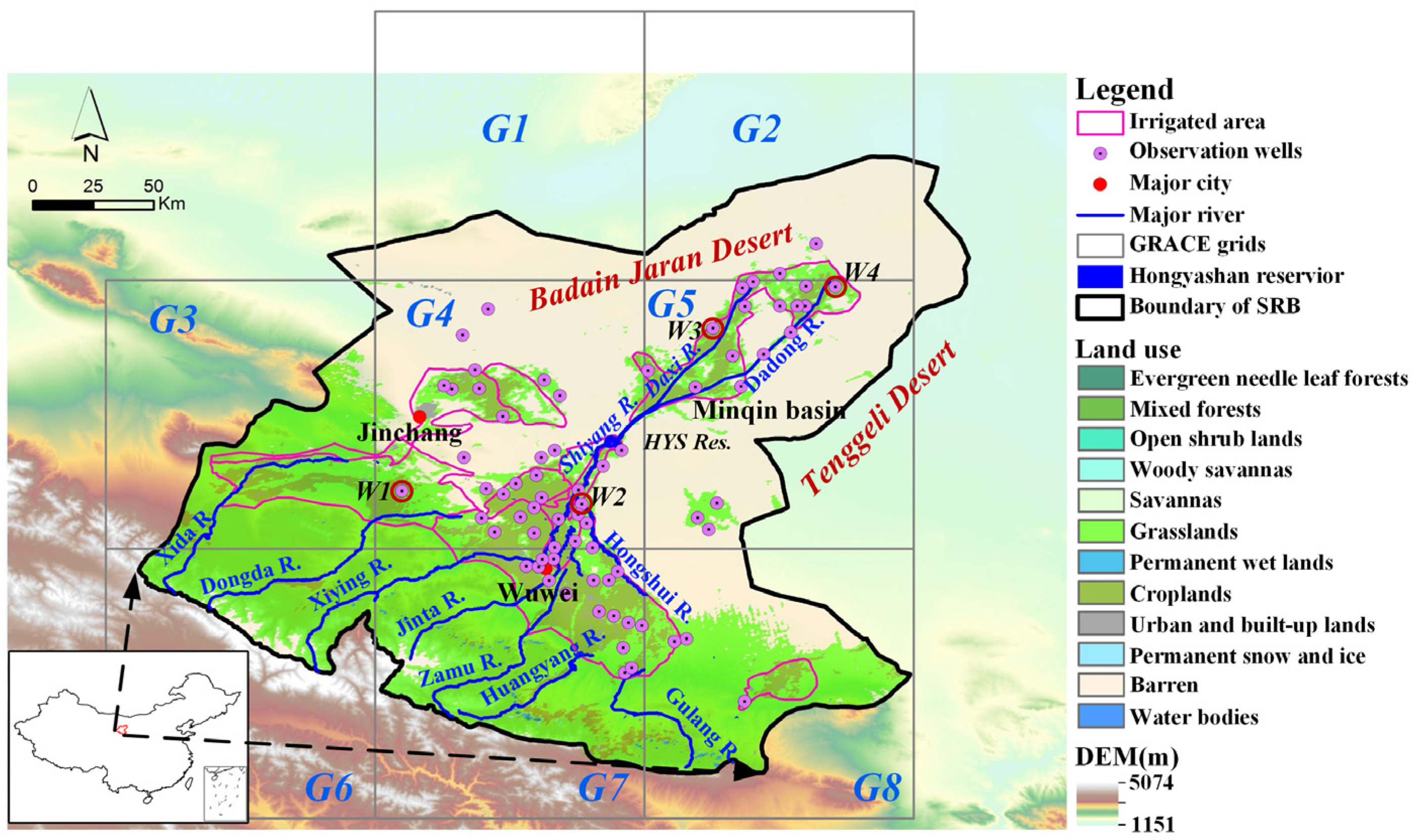
2.1. Study Area

The SRB (Figure 1) is located east of the Hexi Corridor in China and north of the Qilian Mountains, between 36~42 degrees north latitude and 101~104 degrees east longitude. The SRB is surrounded by two deserts to the east, west and north, i.e., the Tenggeli and Badain Jaran deserts, which are typical desert oases, with a total area of 41,600 km². The terrain is high in the south and low in the north, tilting from the southwest to the northeast, and land-use classes in the SRB mainly include croplands, barren land and grasslands, accounting for approximately 10%, 49%, and 41% of the area, respectively. The entire basin can be divided into four geomorphic units: the southern Qilian Mountains, central corridor plains, northern hilly areas and desert areas. In the southern Qilian Mountains, which are 2000~5000 m above sea level, the mountains generally trend from the northwest to the southeast. The central corridor plain area is divided into northern and southern basins by the Hanmu Mountain, Hongya Mountain and Alagu Mountain. The southern basin includes the Dajing, Wuwei and Yongchang sub-basins with elevations ranging from 1400 m to 2000 m. The northern basin includes the Minqin subbasin and Jinchuan-Changning sub-basin with elevations of 1300~1400 m. The lowest elevation is in Baitinghai at only 1020 m. The low hilly area in the north has an altitude of less than 2000 m. The SRB is located deep within the hinterland of the mainland and has a continental temperate arid climate. Climatic characteristics include strong solar radiation, sufficient sunshine, a large temperature difference, low precipitation, strong evaporation and dry air. Precipitation in the SRB is mainly concentrated in the Qilian Mountains. Precipitation in mountainous areas is abundant and relatively stable annually. The average annual precipitation is 300~600 mm, which not only provides good growth conditions for forests and grasslands in mountainous areas, but also reliably guarantees water resources in the plain areas. Precipitation in the plain areas is low, with an average annual value of 200 mm. The basin water system mainly originates in the Qilian Mountains. From east to west, there are seven main rivers and many small ditches and rivers, including the Gulang River, Huangyang River, Zamu River, Jinta River, Xiying River, Dongda River and Xida River, which flow from southwest to northeast. Precipitation in the mountainous areas and melting water from alpine ice and snow are the main water supplies for the rivers. The aquifer system in the study area is mainly composed of the Quaternary porous aquifer system, which varies from the unconfined sand layer in the upper part of SRB to being multi-layered in the middle and lower section of the SRB [24]. For many years, the dynamic characteristics of groundwater in the SRB have included the continuous decline in the groundwater level. From the data investigated by Management Bureau of Shiyang River Basin of Gansu, the last 20 years, from 1980 to 2000, show that the groundwater level in the South Wuwei Basin has decreased by 6~7 m, the rate of decline has been 0.31 m/year, and in the Minqin Basin, the decrease has shown an average of 10~12 m, with a decline of 0.57 m/year, and the maximum decrease being 15~16 m. At the beginning of the 21st century, the consumption rate of water resources in the basin reached 109%, and the development and utilization of water resources reached 172%, which is far more than the reasonable carrying capacity of the water resources in the basin. The superposition of resource-based and structural water shortages has led to the deterioration of the ecological environment of the basin, such as the decline in the groundwater level, disappearance of lakes, acceleration of land desertification and salinization, and the death of natural vegetation in large areas. If the Minqin oasis disappears, the western part of China will face the threat of desert erosion. Therefore, the ecological environment of the SRB has been highly valued by the state and is widely considered by all sectors of society.

2.2. Methods

The flowchart for this study is shown in Figure 2. First, different data sources will be collected, and the GRACE-GLDAS-derived GWS will be validated using in situ groundwater data. Then, the changes in GWS and TWS will be discussed in detail, and combined with remote-sensing and observation data, the causes of GWS changes will be explained. Finally, groundwater storage variation under the influence of human activities will be further analyzed using the water balance equation.

2.2.1. Principle of Terrestrial Water Balance

According to the principle of water balance, important factors, such as precipitation (P), actual evapotranspiration (ET), runoff (R) and human activity influence (Q), may contribute to the variation in water storage in the SRB with intense human activities. The terrestrial water storage change (TWSC) can be expressed as Equation (1) [25]:

$$\frac{ds}{dt}=P-ET-R-Q$$

(1)

where ds/dt means the change in terrestrial water storage with the given time (t).

Given that other items are known, the influence of human activities can be isolated as:

$$Q=P-ET-R-\frac{ds}{dt}$$

(2)

GRACE-based TWSC is calculated as the backward difference of the TWSA [26] as:

$$\frac{ds}{dt}=\frac{TWSA\left(t\right)-TWSA\left(t-1\right)}{t}$$

(3)

2.2.2. Terrestrial Water Storage Variations

There are two main processing approaches for GRACE data: Parameterizing the Earth’s gravity field using global spherical harmonics (SH) basis functions and parameterizing the gravity field with regional mass concentration functions (mascons). Spherical harmonic and unconstrained mascon data are similar as they are both based on the same fundamental GRACE satellite data and models that remove atmospheric, oceanic, and tidal signals. A basic difference between SH and mascons is that SH solutions are global, whereas mascons can be applied at regional to global scales [27]. In this study, we used the monthly 0.5° GRACE level-3 mascon (mass concentration) datasets from the RL06 time-variable gravity field model provided by the Jet Propulsion Laboratory (JPL) (ftp://podaac-ftp.jpl.nasa.gov/allData/tellus/L3/landmass/RL06 (accessed on 18 March 2021)). The C20 coefficients were replaced with the solutions from satellite laser ranging [28], and the degree-1 coefficients were estimated using the method from Swenson et al. [29]. A glacial isostatic adjustment correction was applied for the JPL mascon based on the ICE6G-D model from Peltier et al. [30], and the data are presented as anomalies relative to the time-mean baseline of the period from January 2004 to December 2009. The gridded products used in this paper covered a total period of 173 months, spanning from January 2003 to December 2019. Data from 31 months during the study period are not available. The missing data during the period from July 2017 to May 2018 were due to the discontinuation of GRACE and GRACE-FO satellite data, and the other 20 months were interpolated by simply averaging the values of the two months before and after the month with the missing data [31]. For the consistency of data resolution, the 0.5° of GRACE data was averaged to 1°.

2.2.3. Groundwater Storage Variations

Variations in TWS included a vertically integrated measure of water storage changes in groundwater (GW), soil moisture (SM), surface water (SW) and snow water (SWE) (Equation (4)). Therefore, GWS variations can be isolated from TWS components when other components are known. $\Delta GWS$ can be calculated by removing the storage anomaly of the aboveground part from $\Delta TWS$ in accordance with Equation (5):

$$\Delta TWS=\Delta GWS+\Delta SW+\Delta SM+\Delta SWE$$

(4)

$$\Delta GWS=\Delta TWS-\Delta SW-\Delta SM-\Delta SWE$$

(5)

Since reliable and spatially continuous measurements of soil moisture were not currently available throughout our study area, the outputs from land-surface models were used to provide SM and SWE [32,33]. The surface water we used was plant canopy surface water from the land-surface models.

2.2.4. GLDAS Model Data

GLDAS was developed by NASA’s Goddard Space Flight Center and the National Centers of Environmental Prediction (NCEP). The goal of GLDAS is to ingest satellite and ground-based observational data products using advanced land-surface modelling and data assimilation techniques to generate optimal fields of land-surface states and fluxes [34]. The GLDAS-2 datasets consist of 0.25° × 0.25° Noah model data, covering the period from 2000 to the present. The temporal resolution for the GLDAS products was three hours. Monthly products were generated through temporal averaging or a summation of the three-hourly products [35]. The GLDAS data were retrieved from http://disc.gsfc.nasa.gov/hydrology/data-holdings (accessed on 12 March 2021). Noah was selected as the data source in this paper, which simulates changes in water storage with less bias and uncertainty than other models in GLDAS [36,37]. The dataset contained soil moisture, snow water equivalent, runoff, plant canopy surface water and ET at a spatial resolution of 0.25° and 1° and a temporal resolution of three hours or one month. For consistency with the GRACE data, the average SM, SWE and plant canopy anomalies versus time were computed.

2.2.5. Precipitation Data

This study mainly collected two precipitation products: TRMM and CMA datasets. TRMM (Tropical Rainfall Measuring Mission, TRMM 3B43, 1998–2019) provided the temporal and spatial distribution and changes in precipitation in the range of 50° south latitude to 50° north latitude, with a spatial resolution of 0.25°. The monthly precipitation dataset (0.5°) in China from January 1980 to December 2019 was obtained from the China Meteorological Administration (CMA), which integrated the daily precipitation observed by 2472 national stations (including the National Climate Observatory and the first-level and second-level meteorological observation stations) and adopted the optimal interpolation method based on the climate background field, in order to generate the grid product of daily precipitation in China.

2.2.6. ET Data

The ET data used in this study included actual ET from the GLEAM, MODIS and GLDAS-Noah models. The Global Land Evaporation Amsterdam Model (GLEAM) is a set of algorithms dedicated to the estimation of terrestrial evaporation and root-zone soil moisture from satellite data. Since its development in 2011, the model has been continuously revised and updated [38]. To date, three kinds of datasets produced using the latest version of GLEAM v3.5 are currently available, and the three v3.5 datasets differ only in their forcing and spatial coverage (http://www.gleam.eu (accessed on 1 March 2021)). GLEAM v3.5a is a global dataset spanning the 39-year period, 1980~2020, at a 0.25° spatial resolution. For more detailed information about GLEAM data, see the previous study by Miralles et al. [39].

The actual MODIS/MOD16 ET datasets were estimated according to the Penman-Monteith equation [40]. Mu et al. [41,42] modified the MODI6 actual ET algorithm several times in order to improve the accuracy of ET components, including night time ET, canopy transpiration, and soil heat flux, which has been successfully used in many regions worldwide. Previous studies have assessed the accuracy of MOD16 ET in several river basins in China [43,44]. The results showed that the fitting effect improved at the station scale, with an average correlation coefficient of 0.76. The monthly actual mean ET at a spatial resolution of 1 km was averaged for different spatial resolutions over the period 2003–2019.

2.2.7. Land-Cover Data from MODIS

The MODIS land-cover type product (MCD12Q1) provides a suite of science datasets (SDSs) that map global land coverage at a 500 m spatial resolution at annual time steps for six different land-cover legends, and was produced using supervised classification techniques, such as decision trees [45] and ensemble classification methods [46]. The product contains 13 science datasets, including five legacy classification schemes (IGBP, UMD, LAI, BGC, and PFT) and a new three-layer legend based on the Land Cover Classification System (LCCS) from the Food and Agriculture Organization [47], and the dataset we used to analyze land-use change in the study area is the IGBP classification scheme. More details can be found at https://doi.org/10.5067/MODIS/MCD12Q1.006 (accessed on 5 March 2021).

2.2.8. Mutation Test Methods

We used two mutation test methods to analyze the mutation characteristics of the GWSA trend in the SRB.

Mann-Kendall Nonparametric Mutation Test

The Mann-Kendall [48,49] mutation test [50] is a nonparametric statistical test method. Its advantage is that it is not only easy to calculate, but it can also clarify the starting point of the mutation and can identify the mutation period; it is commonly used for trend analysis and variation testing of hydrological and meteorological elements, such as rainfall, temperature and runoff. For time series x with n sample sizes, the rank column S_k of the sequence needs to be constructed in the following manner:

$${\mathrm{S}}_k={\displaystyle \sum }_{i=1}^k{r}_i$$

(6)

$$r_i=\{\begin{array}{l}1, if x_i>x_j\\ 0, else\end{array}\left(j=1,2,\dots ,i\right)$$

(7)

where S_k is the cumulative number of values at moment i, which is greater than that at moment j. Under the assumption of a random and independent time series, the following statistics can be determined:

$$U{F}_k=\frac{\left[S_k-E\left(S_k\right)\right]}{\sqrt{Var\left(S_k\right)}}\left(k=1,2,\dots ,n\right)$$

(8)

where $U{F}_1=0$, $E\left(S_k\right)$ and $Var\left(S_k\right)$ are the mean and variance of $S_k$, respectively. When $x_1$, $x_2$, and $x_n$ are independently and continuously distributed, they can be calculated by the following equations:

$$E\left(S_k\right)=\frac{n\left(n-1\right)}{4}$$

(9)

$$Var\left(S_k\right)=\frac{n\left(n-1\right)\left(2n+5\right)}{72}$$

(10)

where $U{F}_i$ is a standard normal distribution. For a given significance level, the critical value $U_a$ can be obtained by querying the normal distribution table. If |$U{F}_i$| > $U_a$ ($U_{0.05}$ = 1.96, $U_{0.01}$ = 2.58), it indicates that the sequence has an obvious trend of increasing or decreasing. The time series x is generated into its corresponding inverse sequence The calculation process above is repeated to obtain the inverted sequence statistical value $U{B}_k$ ($U{B}_k$ = $-U{F}_k,k=n,n-1,\dots ,1,U{B}_1=0$). When the $U{F}_k$ and $U{B}_k$ curves intersect between the critical boundary, the intersection point can be used as the beginning of the mutation [51].

Moving T-Test Method

The moving T-test assumes that the front of the sliding point is sequence 1 and the rear of the sliding point is sequence 2. The samples with capacities of $n_1$ and $n_2$ are extracted from the two sequences, and the assumption that the distribution functions of the two sequences are equal is tested:

$$T=\frac{{\overline{x}}_1-{\overline{x}}_2}{S_w{\left(\frac{1}{n_1}+\frac{1}{n_2}\right)}^{\frac{1}{2}}}$$

(11)

$$S_w{}^2=\frac{\left(n_1-1\right)S_1{}^2+\left(n_2-1\right)S_2{}^2}{n_1+n_2-2}$$

(12)

$$S_1{}^2=\frac{1}{\left(n_1-1\right)}{{\displaystyle \sum }}_{t=1}^{n_1}{\left(x_t-{\overline{x}}_1\right)}^2$$

(13)

$$S_2{}^2=\frac{1}{\left(n_2-1\right)}{{\displaystyle \sum }}_{t=n_1+1}^{n_1+n_2}{\left(x_t-{\overline{x}}_2\right)}^2$$

(14)

where ${\overline{x}}_1$ and ${\overline{x}}_2$ are the mean values of the two samples and T obeys a $T\left(n_1+n_2-2\right)$ distribution. For a given significance level a, the original assumption is rejected when $\left|T\right|>{\mathrm{t}}_{a/2}$, the two samples have a significant difference and the sequence is mutated.

2.2.9. Correlation Analysis and Data

This study used correlation analysis to study the relationship between different variables. The results are expressed by the correlation coefficient r, which is used to describe the strength of the linear correlation between two variables. The formula is as follows:

$$r=\frac{{{\displaystyle \sum }}_{i=1}^n\left(X_i-\overline{X}\right)\left(Y_i-\overline{Y}\right)}{\sqrt{{{\displaystyle \sum }}_{i=1}^n{\left(X_i-\overline{X}\right)}^2}\sqrt{{{\displaystyle \sum }}_{i=1}^n{\left(Y_i-\overline{Y}\right)}^2}}$$

(15)

where $X_i$ and $Y_i$ are sample values and $\overline{X}$ and $\overline{Y}$ are the mean values of the sample values, respectively.

The data used in this study are listed in

Table 1. Data sources used in this study.

Items	Spatial Resolution	Temporal Resolution	Time Span
TWSA from GRACE	0.5°	Monthly	2003–2019
CMA	0.5°	Monthly	2003–2019
TRMM 3B43	0.25°	Monthly	2003–2019
ET, SWE, SM, Plant canopy surface water and Runoff from NOAH_2.1	1°	Monthly	2003–2019
MODIS ET	1 km	Monthly	2003–2019
GLEAM ET	0.25°	Monthly	2003–2018
Land cover from MODIS	0.05°	Yearly	2003–2019
Groundwater observation wells	—	Monthly	2007–2018

.

3. Results and Discussion

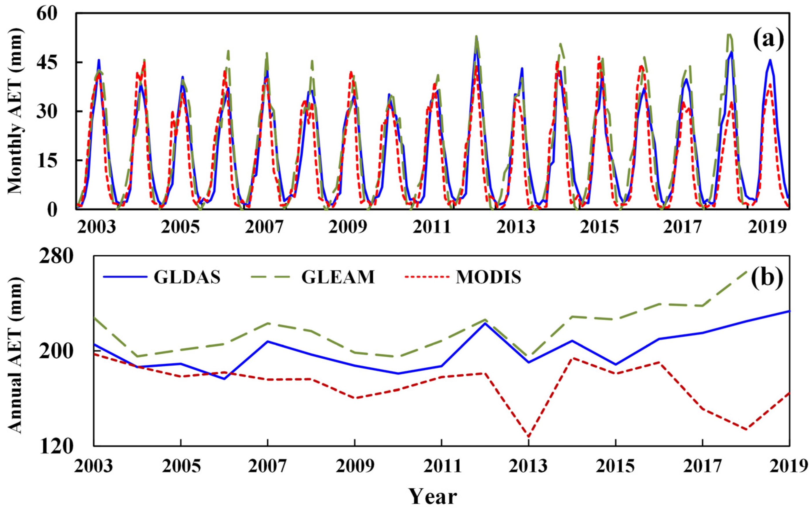
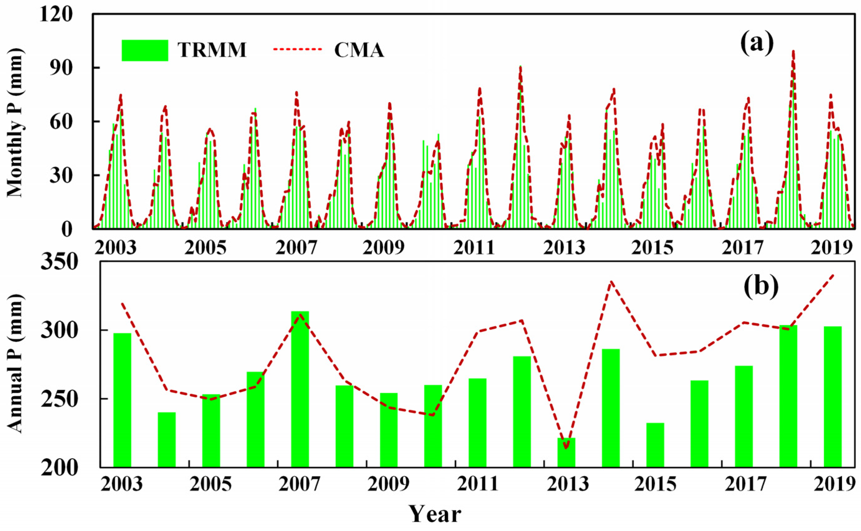
3.1. Changes in Precipitation and Actual Evapotranspiration in the SRB

Figure 3 shows monthly and yearly average changes in precipitation from the TRMM and CMA datasets in the SRB. The two datasets have a high consistency, with a correlation coefficient of 0.97 at the monthly scale and an RMSE (root mean square error) of 6.18 mm/month, and the TRMM data show a 10 mm underestimation in the rainy season at the monthly scale. The yearly precipitation in the SRB showed a fluctuation at a small magnitude of 50 mm from 2003 to 2015. However, precipitation showed an obvious upward trend after 2015, with an average annual precipitation of 276 mm. Precipitation in the rainy season accounts for 70% of the annual value. Due to the high consistency of the two sets of data and the higher resolution of the TRMM dataset than that of the CMA dataset, TRMM data was chosen for the subsequent analysis. To facilitate the comparative analysis with GRACE data, the resolution of precipitation data was upscaled to 1°.

Figure 4 plots the monthly and annual average actual ET changes from three kinds of data sources (GLEAM, MODIS and GLDAS-Noah models) over the period from 2003 to 2019 in the SRB. Generally, the actual ET changes in the three datasets are consistent with a correlation coefficient of above 0.8. The actual ET from the three datasets hits a peak in the period from June to August and reaches a trough in December and January, showing a significant seasonal trend. Compared to the GLEAM and GLDAS-Noah model data, the monthly MODIS-ET data had a slight underestimation of the peak and are significantly smaller than the other two datasets on an annual scale. The annual average actual ET from the three products showed a similar pattern from 2003 to 2014, showing a downward trend from 2003 to 2005 and from 2007 to 2009, and rising after 2009. The MODIS-ET data was significantly different from the GLEAM and GLDAS-Noah model ET data after 2016. Hence, GLEAM data was chosen for this study. Similarly, to facilitate the analysis of the GRACE data, the actual ET data was upscaled to 1°.

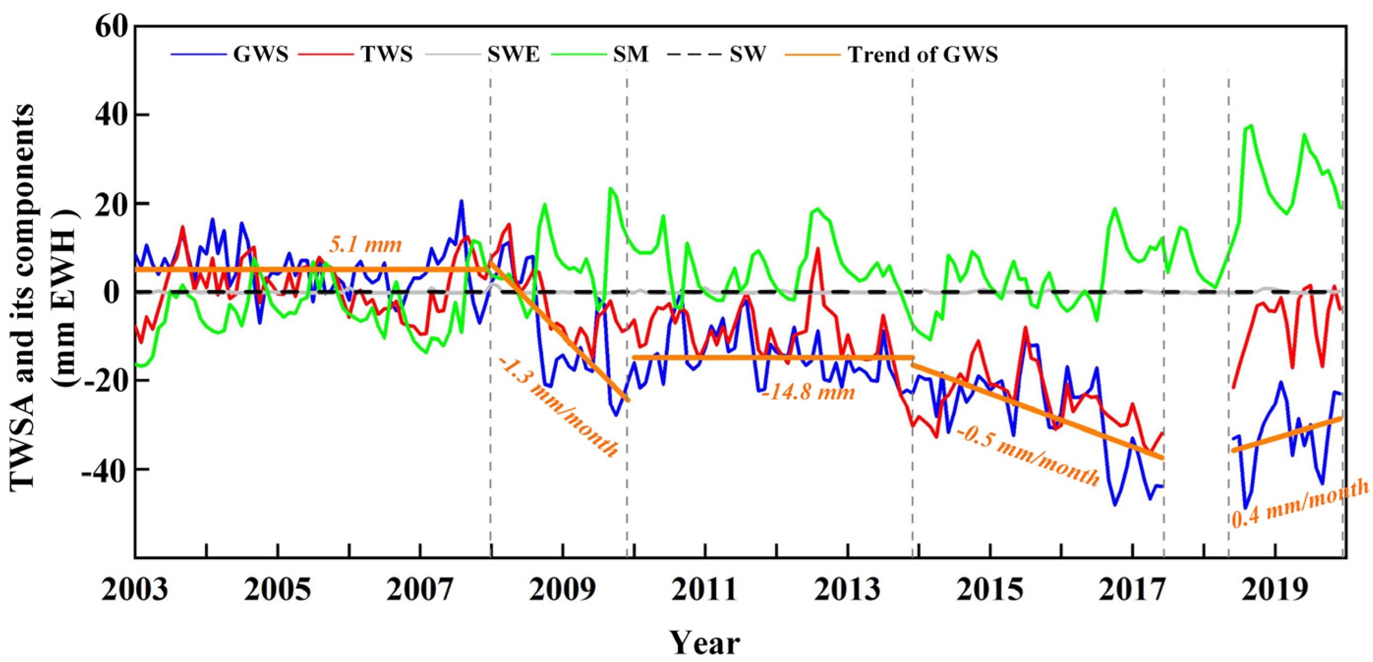
3.2. Variations of TWSA Data and Their Components

Figure 5 shows the variations in TWS retrieved by GRACE, the surface water (SW), soil moisture (SM) and snow water equivalent (SWE) derived from the GLDAS-Noah model, and the GWSA retrieved by the GRACE and GLDAS model data from 2003 to 2019 in the SRB. Overall, the variation in TWS showed a trend that was similar to that of GWS. The variation in GWS in the SRB showed a slight small decreasing trend over the period from 2003 to 2007, with an average GWSA of 5.1 mm EWH. From 2008 to 2009, the average downward rate was −1.3 mm/month. The GWSA from 2010 to 2013 remained stable, with an average value of −14.8 mm EWH. After 2014, the GWS had a downward trend, with a decline of approximately −0.5 mm/month. After 2018, GWS began to rise at a rate of approximately 0.4 mm/month. SM had a slow rising trend from 2003 to 2019, and it accounted for a large proportion of the variations in TWS, while SWE and SW had a small impact on the variations in TWS, except for a small SWE change from December to February in each year (<1 mm EWH), and it fluctuated at approximately zero at other times.

Figure 6 shows the variations in annual TWS, GWS, change in AET (changes in actual evapotranspiration relative to the mean value of 2004–2009), and change in precipitation (changes in precipitation relative to the mean value of 2004–2009) over time in the SRB from 2003 to 2019. The TWS and GWS in the SRB had a declining trend during this period, which is similar to the results obtained by Wang et al. [52] in the Hexi Corridor, and the average declining rates were 1.58 mm/year, and 2.95 mm/year, respectively. The correlation coefficient between TWSA and GWSA was 0.81, indicating that the variation in TWS was well correlated with the variation in GWS in the SRB. Moreover, annual precipitation and actual evapotranspiration in the SRB increased to varying degrees, and the rate of annual actual evapotranspiration was slightly higher than that of the annual precipitation, with rates of 2.55 mm/year, and 1.18 mm/year, respectively. By analyzing the relationship between meteorological factors and water storage, it can be found that, in the years with rapid declines in water storage, such as 2009, 2014, 2016 and 2017, the actual ET was greater than that of the precipitation in the previous year. Due to drought, upstream inflow was reduced, and exploitation increased, which eventually led to a decline in GWS [53]. Using correlation analysis among TWSA, GWSA and the difference between the previous year’s precipitation and ET both show a correlation, and the correlation coefficients are greater than 0.6, indicating that the variation in water storage in the SRB was affected by meteorological factors to some extent.

Surface runoff mainly occurs in the Qilian Mountain area in the upper reaches of the SRB. There are two agricultural irrigated areas (G4 and G5 grid blocks), located in the middle and downstream areas in the SRB, which do not have runoff production. Since the Hongyashan Reservoir was built in 1958, surface water from the Shiyang River into Minqin has been completely controlled by the reservoir, and all the water has been introduced into the area for irrigation.

GRACE-derived GWS changes represent regional groundwater storage change under the ground. However, observations of well data showed a groundwater level change at the point scale. Many researchers have compared GRACE-derived GWS data with in situ measured data [54,55,56], and the correlation coefficients ranged from 0.60 to 0.85. In this study, the daily groundwater level (GWL) in 71 observation wells in the SRB, from January 2007 to December 2018, was recorded, and 18 wells had complete monitoring data, which were mainly concentrated in the middle and lower reaches of the SRB (G4, G5). Therefore, the observation of well data in these two grids were averaged and compared to the GRACE data. Figure 7a shows that the change in the groundwater level in the G4 and G5 grid blocks was basically consistent with the trend in the GRACE data, and the correlation coefficient was 0.68 (p < 0.01). Therefore, we think GRACE-derived GWSA is reasonable and consistent with previous studies, which can reflect the dynamic changes of groundwater in SRB. In addition, by observing the change in the groundwater level in this area, it can be found that the average annual decline in the groundwater level in the middle and lower reaches of the SRB before 2012 was approximately 0.6 m, the change in groundwater level in 2012–2015 was almost stable, and the groundwater level increased significantly after 2015, in which the change was approximately 0.4 m/year. In addition, the groundwater level in the middle and lower reaches of the SRB also showed strong annual fluctuations before 2012. From July to August, the groundwater level reached its lowest level due to irrigation and pumping in spring. From autumn to spring, the groundwater level recovered in the second year due to the decrease in irrigation and pumping, in addition to possible lateral replenishment from rivers [57]. Annual changes in groundwater levels after 2012 were more stable than before. This may have been related to the closure of a large number of drilling wells, the completion of field water savings and cross-basin water transfer and other measures in the key governance project of the SRB, indicating the effect of strengthening groundwater management and implementing strict groundwater control and mining systems. According to the water resource bulletin data of the SRB in 2010, the amount of groundwater extraction in the SRB was 0.61 billion m³, which was 47.6% lower than the value of 1.16 billion m³ in 2006. Furthermore, the amount of water transferred in the SRB was no less than 0.2 billion m³ after 2010, which also played a positive role in curbing the downward trend in groundwater.

Figure 7b–c shows the dynamic changes in groundwater level in the G4 and G5 observation wells. The observation well positions are shown in Figure 1. The groundwater level of each well fluctuated greatly before 2012 and then gradually stabilized, and each well only differed in the amplitude of the water level. Groundwater level fluctuations in monitoring wells near the Shiyang River (W2) in G4 were small, and the amplitude was approximately 1 m. Groundwater level fluctuations in monitoring wells far from the river (W1) were large, which may have been related to the hydraulic connection between the surface and groundwater. The wells near the river easily received river recharge and maintained a stable water level. The groundwater level in the downstream area (G5) had obvious fluctuations before 2012 and then became stable.

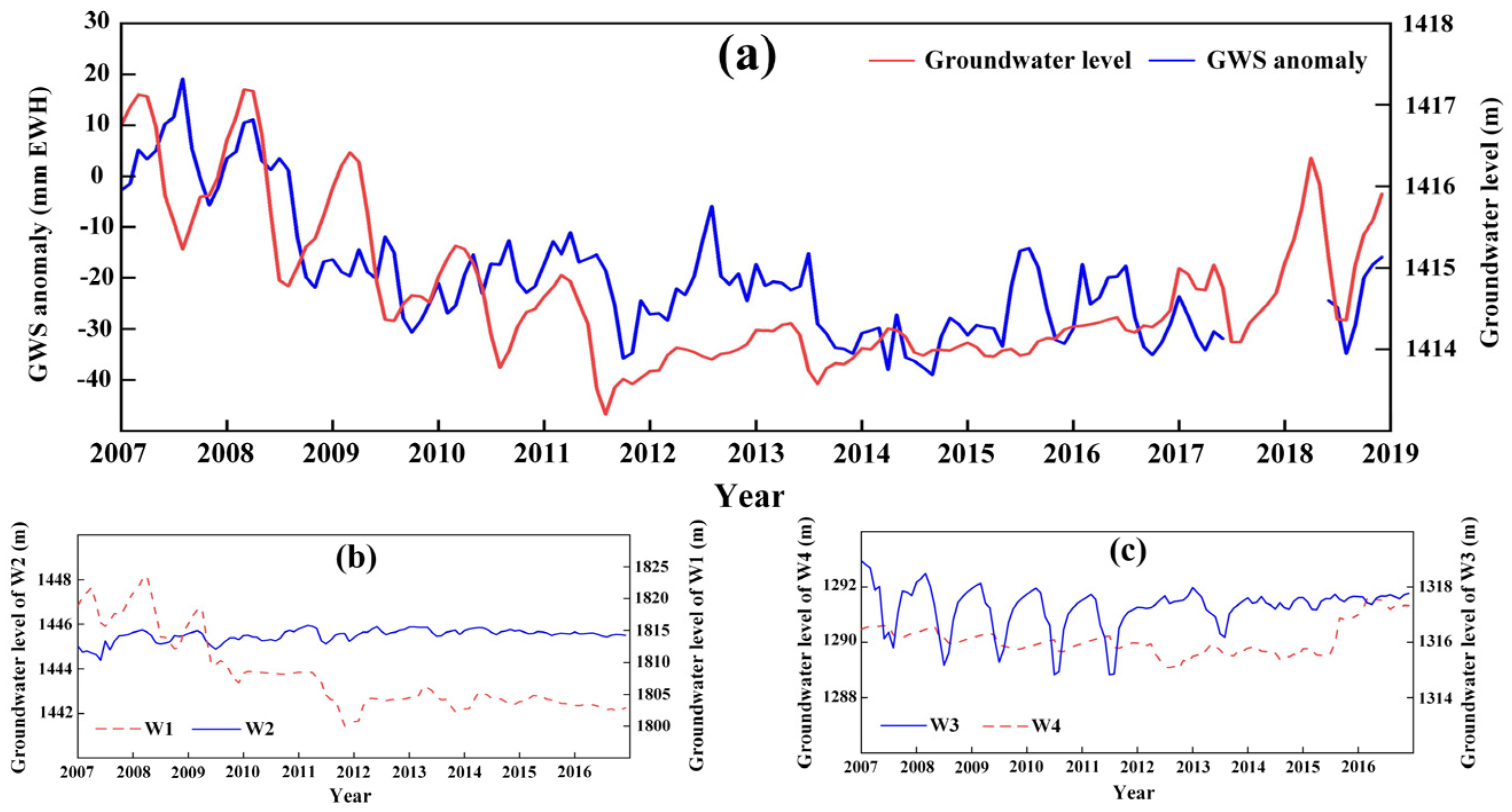
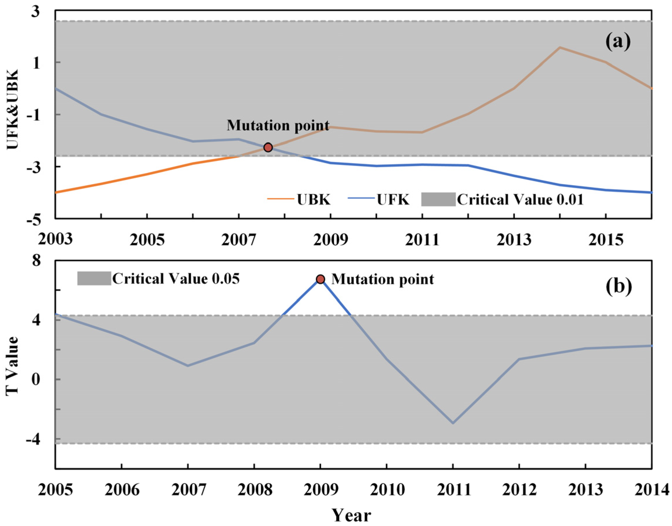
3.3. Abrupt Change in GWS Variations

From the trend of GWS, as of 2016, GWS in the middle and lower reaches of the SRB have been in a downward trend, and the change was −44 mm EWH, as compared to 2003, which is equivalent to a decrease of 8.8 × 10⁸ m³ in GWS and an annual decrease of 0.6 × 10⁸ m³. In addition, the rate of decline in GWS changed significantly before and after 2009, accounting for 1.2 × 10⁸ m³/year, and 0.05 × 10⁸ m³/year, respectively. The M-K mutation test was used to detect the GWS mutation point (Figure 8a). From 2004 to 2016, GWS has been significantly decreasing ($U{F}_k$< −1.96), and there was a possible mutation point from 2007 to 2008. Then, the moving T-test method was used for mutation detection (Figure 8b). The step size was set to two, the significance level was 0.05, and the critical value was 4.303. At this significance level, the maximum absolute value of T appeared in 2009 (p < 0.05); therefore, according to the moving T-test method, a possible mutation point in 2009 was detected. By combining the trends of GWS and the two mutation testing methods, we found that, after a series of management plans in the SRB, the decline in GWS was curbed close to 2009.

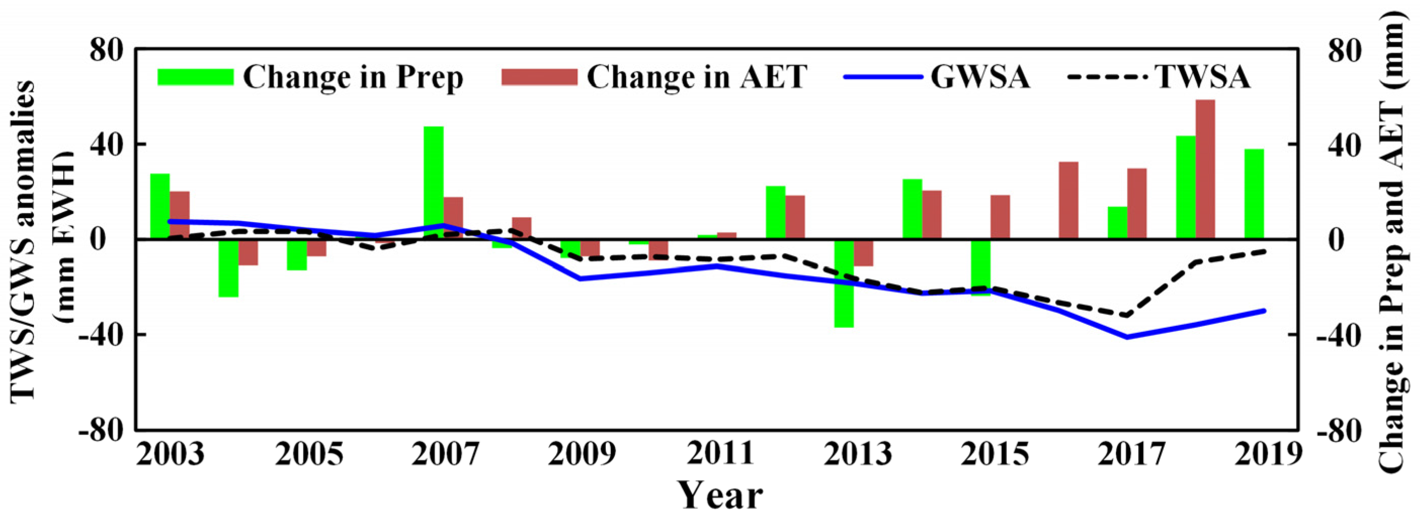
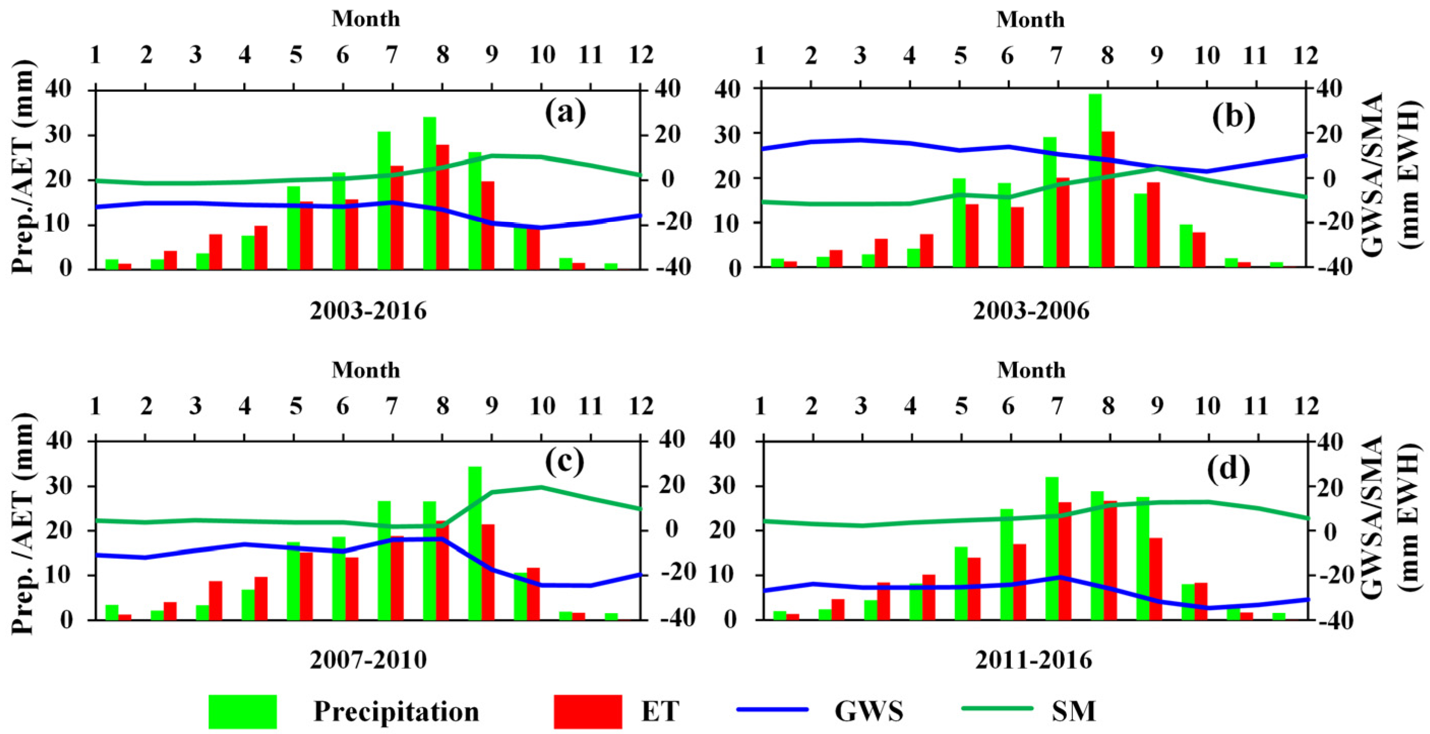
3.4. Evaluation of the Water Balance before and after the Key Management Plan

From the change in GWS in each governance stage (

Table 2. The change in GWS in the middle and lower reaches of the SRB in each governance stage. The water volume is calculated by multiplying the area of the middle and lower reaches of the SRB (20,000 km²).

Period	Change of GWS During the Period		Change Rate
	Equivalent Water Height	Water Volume
2003–2006	−17.9 mm	−3.58 × 108 m3	−4.5 mm/year
2007–2010	−24.3 mm	−4.86 × 108 m3	−6.1 mm/year
2010–2016	−2.2 mm	−0.44 × 108 m3	−0.3 mm/year
2016–2019	9.1 mm	1.82 × 108 m3	2.3 mm/year

), it can be seen that GWS still decreased by 24.3 mm EWH after the end of the first stage of governance (2007–2010). With further strengthening of governance, GWS decreased by 2.2 mm EWH in 2011–2016, which was 91% lower than that in 2007–2010; and by 2019, GWS increased by 9.1 mm EWH, as compared to 2016. After the completion of the water diversion project from the Xiying River to downstream of Minqin, known as the Caiqi Special Water Diversion Canal, 1.33 × 10⁸ m³ and 1.35 × 10⁸ m³ of water was transferred to Minqin and Caiqi in 2010 and 2011, respectively, which greatly increased the inflow to the Minqin Basin. In addition, on the basis of data from 2010, water-saving reconstruction projects were further carried out in the Huangyang, Gulang, Donghe and Qinghe irrigation areas, which effectively improved the water utilization coefficient of irrigation channels and the utilization efficiency of water resources [58].

The monthly average GWSA in the middle and lower reaches of the SRB from 2003 to 2016 were calculated. As shown in Figure 9a, the loss of GWS in the middle and lower reaches of the SRB was the least in July and the most in October. Variations in GWS from January to June were relatively close, and from July to October, the decline in GWS intensified; after October, the sharp decline in GWS was gradually alleviated. In addition, the change in SM in the middle and lower reaches was significantly negatively correlated with the change in GWS (r = −0.9). Under the influence of the rainy season and agricultural irrigation, soil water reserves reached a high value from September to October, while groundwater reserves decreased due to lagging exploitation and irrigation recharge.

The monthly changes in groundwater storage before (2003–2006), during (2007–2010) and after (2011–2016) the SRB key management plan are shown in Figure 9b–d. GWS in the middle and lower reaches of the SRB had a downward trend from March to October in 2003–2006. After the implementation of the SRB management plan in 2007, groundwater exploitation was restricted. With little change in annual precipitation and evapotranspiration, the change in GWS from January to August was more stable than before, but from August to October, GWS still had an obvious downward trend. After 2011, the standard deviation of the monthly changes in GWS became 4.3 mm EWH, which was a little lower than the 7.4 mm EWH for the period from 2007 to 2010.

The influence of human activities calculated by the water balance equation was compared to groundwater extraction from the water resource bulletin of the SRB (Figure 10). Since the human impact calculated by the water balance is expressed as the equivalent water height, the water volume can be converted by multiplying the area of the middle and lower reaches of the SRB (20,000 km²). As shown in Figure 10, the influence of human activities had an upward trend before 2007 and then began to decline, which is consistent with the change in the extraction recorded in the water resource bulletin. After 2010, the extraction of groundwater in the SRB was basically stable at 8 × 10⁸ m³/year, while the human influence obtained by the water balance equation still showed a downward trend after 2010, and the human influence estimated by the water balance was greater than the groundwater depletion, which may have been related to the implementation of water-saving renovation projects and industrial structural deployment in the irrigation area. Due to the large number of drilling wells in the study area, there may have been some wells that were not installed in metering facilities, which may have also led to the results deviation in the bulletin. In addition, the spatial resolution of the impacts from human activities obtained by the water balance method is low, and there may be large errors when applied to small-scale areas such as the SRB. In addition, the error of human influence using different remote-sensing data is about 20%. However, the overall trend still shows that the reduction in water storage, caused by human activities, was effectively reduced by implementing a series of governance activities in the SRB.

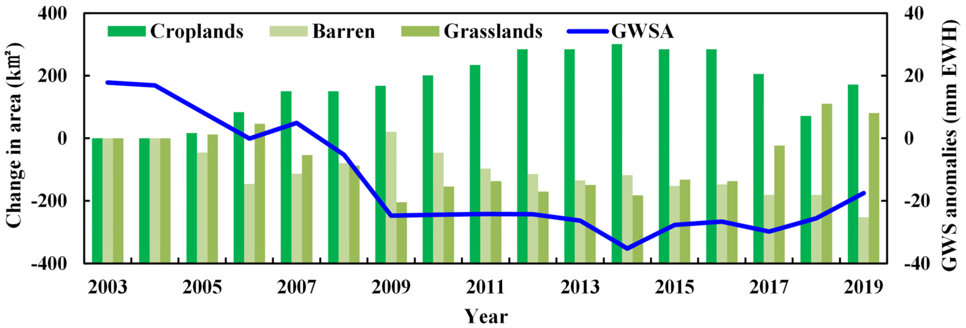
3.5. Land-Use Changes in the Middle and Lower Reaches of the SRB

According to the land-use class changes in the middle and lower reaches of the SRB from MODIS (Figure 11), the cropland area in the middle and lower reaches showed an increasing trend from 2003 to 2016, with a growth rate of 50.2 km²/year from 2004 to 2007. After the implementation of the key management project in 2007, the growth rate of cropland areas in the middle and lower reaches decreased significantly. The growth rates from 2007 to 2016 were 16.8 km²/year (2007–2010) and 13.9 km²/year for 2010–2016. After 2016, the cropland area decreased significantly, and the change rate was −106.6 km²/year. By analyzing the variation of GWS in the middle and lower reaches, it can be found that the variation of GWS had a strong negative correlation with the change in cropland area, and the correlation coefficient was −0.94 (p < 0.01), indicating that the variation in GWS in the middle and lower reaches was closely related to cropland cultivation; reducing cropland areas had a significant effect on restoring GWS. With the decrease in cropland area and the rise in GWS, the barren area in the middle and lower reaches was gradually reduced, and natural vegetation, such as grassland, was gradually restored, indicating that the ecosystems in the SRB were in a recovery stage [59].

4. Conclusions

To understand the influences on water resources of the implemented key governance project of the Shiyang River Basin in 2007, this article studied the changes in terrestrial water and groundwater storage from 2003 to 2019. GRACE-GLDAS data were used to quantitatively evaluate the changes in groundwater storage before and after the SRB key management project. Combined with precipitation, actual ET, land use, bulletin and in situ observation data, the natural and human factors affecting the changes in water storage were analyzed, and the situation of ecological restoration in the SRB was evaluated from the perspective of water resources. The conclusions are as follows:

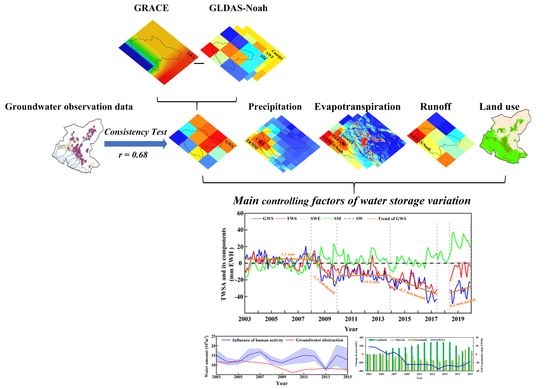
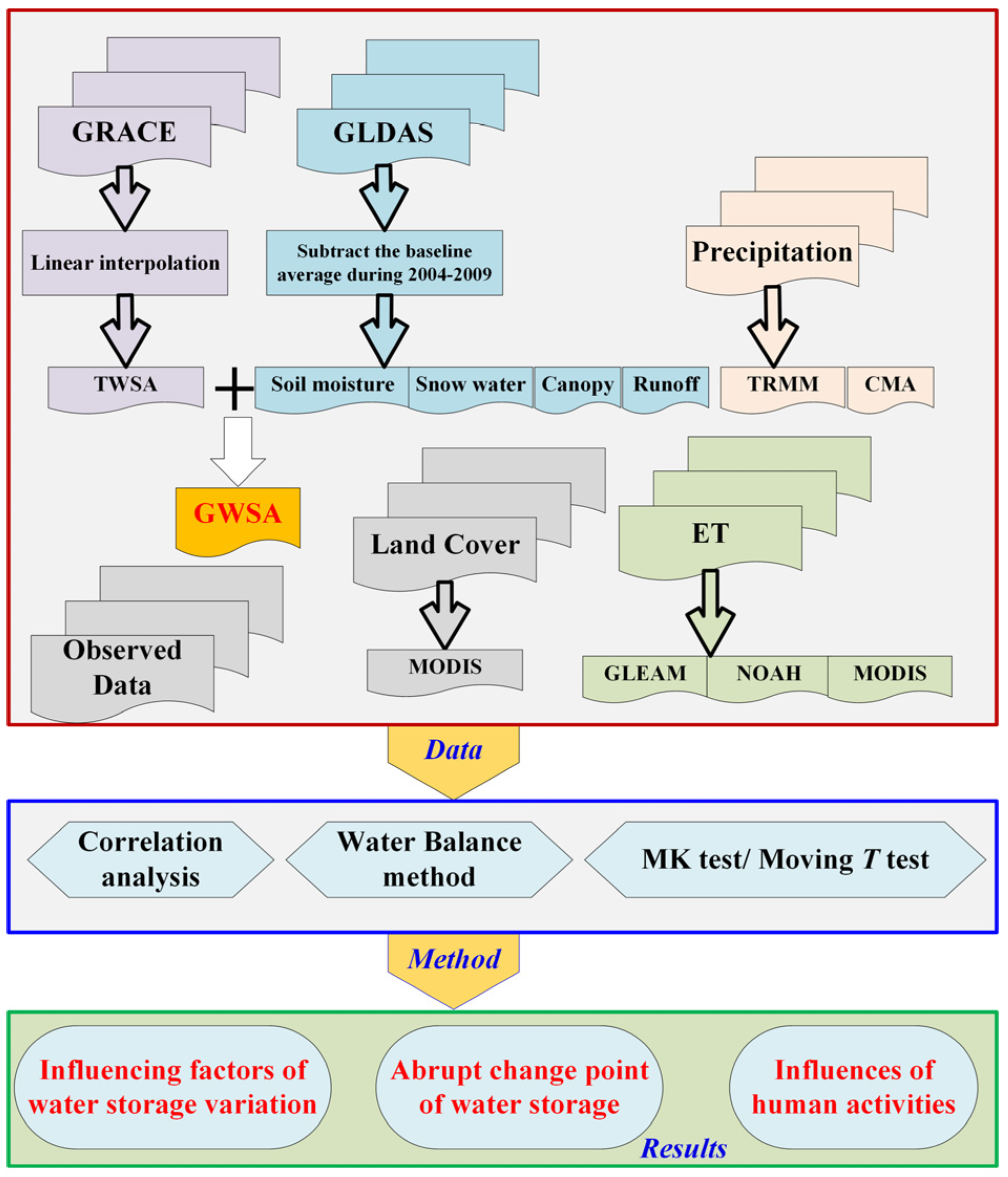
• The variation in GWS obtained by GRACE and GLDAS was compared to the data from groundwater observation wells, and the results from the two sources show consistency of the wells (r = 0.68), indicating that the GRACE was reliable for GWS monitoring in the SRB. GWS in the SRB had a slow downward trend from 2003 to 2016. After 2018, GWS increased by approximately 0.4 mm/mon, which was approximately 3.84 × 10⁸ m³ per year. Additionally, the GRACE-observed TWSA was fairly well-correlated with the GWSA (r = 0.81).
• Different datasets of precipitation and actual ET data in the SRB were used to analyze their relationship with the GWSA. There was a correlation between the variation in GWS in the current year and the difference between precipitation and actual ET change in the previous year (r = 0.61). From 2003 to 2006, due to the increase in precipitation, GWS remained stable, and from 2007 to 2009, due to the decrease in precipitation and the increase in cropland area, GWS decreased significantly. The downward trend of GWS was curbed near 2009, and the rate of decline after 2009 was 96% lower than that before 2009. From 2011 to 2016, GWS in the middle and lower reaches of the SRB decreased by approximately 0.44 × 10⁸ m³, which is 91% less than that of 4.86 × 10⁸ m³ from 2007 to 2010.
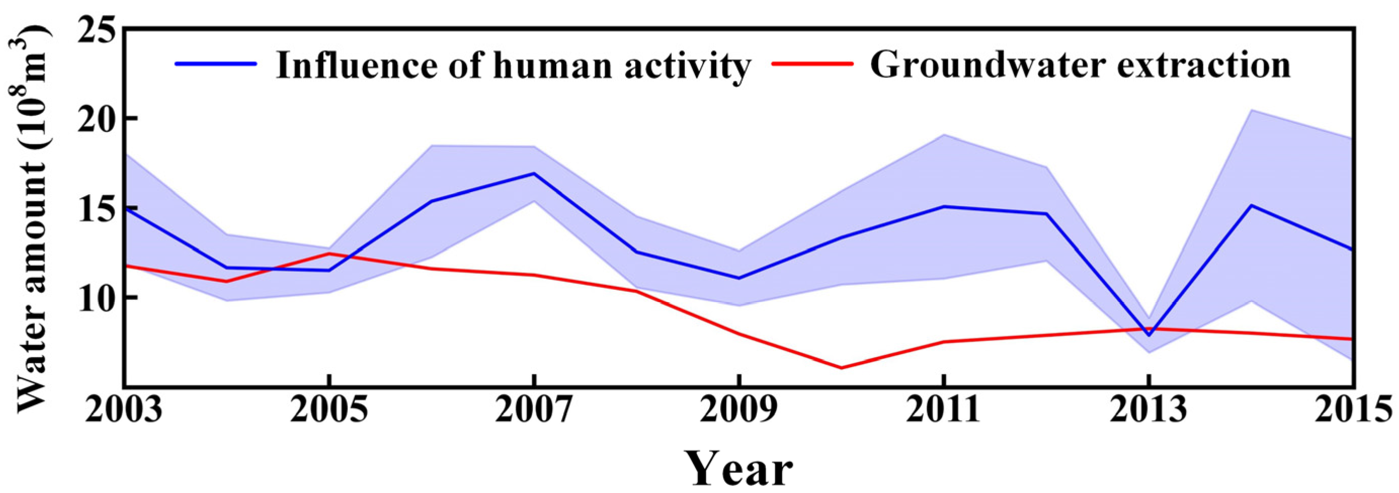
• By using the water balance method, the change in GWS affected by human activities was obtained, and the influencing factors were discussed. The change in GWS affected by human activities rose before 2007 and then decreased, which was consistent with the change in groundwater depletion in the SRB. Land-use change in the middle and lower reaches of the SRB also showed that the increasing rate of the crop area gradually slowed down after 2011 and significantly decreased after 2016. Natural vegetation areas gradually increased, and GWS also gradually rose, which indicated that, through a series of governance activities in the SRB, the reduction in water storage caused by human activities was effectively reduced, and the ecological environment of the SRB gradually recovered.

GRACE/GRACE-FO data could provide accurate estimation of regional groundwater storage changes to support groundwater resource management. In desert and remote areas, GRACE is the only means to evaluate groundwater reserve change. However, due to the coarse resolution of GRACE data, the applicability of GRACE-derived GWSA data in small-scale areas should be explored. In addition, the uncertainties in multisource remote-sensing data used in the principle of water balance may also affect the accuracy of human impacts. However, in the absence of groundwater extraction data, multi-source remote-sensing data and water balance methods can provide feasible solutions for assessing the impact of human activities on groundwater storages.

References

1. Oki, T.; Kanae, S. Global Hydrological Cycle and World Water Resources. Science 2006, 313, 1068–1072. [Google Scholar] [CrossRef] [PubMed] [Green Version]
2. Kundzewicz, Z.W.; Doell, P. Will groundwater ease freshwater stress under climate change? Hydrogeol. Sci. J. 2009, 54, 665–675. [Google Scholar] [CrossRef] [Green Version]
3. Scanlon, B.R.; Longuevergne, L.; Long, D. Ground referencing GRACE satellite estimates of groundwater storage changes in the California Central Valley, USA. Water Resour. Res. 2012, 48, 48. [Google Scholar] [CrossRef] [Green Version]
4. Famiglietti, J.S. The global groundwater crisis. Nat. Clim. Chang. 2014, 4, 945–948. [Google Scholar] [CrossRef]
5. Konikow, L.F.; Kendy, E. Groundwater depletion: A global problem. Hydrogeol. J. 2005, 13, 317–320. [Google Scholar] [CrossRef]
6. Su, Y.Z.; Zhao, W.Z.; Su, P.X.; Zhang, Z.H.; Wang, T.; Ram, R. Ecological effects of desertification control and desertified land reclamation in an oasis–desert ecotone in an arid region: A case study in Hexi Corridor, northwest China. Ecol. Eng. 2007, 29, 117–124. [Google Scholar] [CrossRef]
7. Long, D.; Yang, W.; Scanlon, B.R.; Zhao, J.; Liu, D.; Burek, P.; Pan, Y.; You, L.; Wada, Y. South-to-North Water Diversion stabilizing Beijing’s groundwater levels. Nat. Commun. 2020, 11, 1–10. [Google Scholar] [CrossRef]
8. Sun, W.; Jin, Y.; Yu, J.; Wang, G.; Xue, B.; Zhao, Y.; Fu, Y.; Shrestha, S. Integrating satellite observations and human water use data to estimate changes in key components of terrestrial water storage in a semi-arid region of North China. Sci. Total Environ. 2020, 698, 134171. [Google Scholar] [CrossRef] [PubMed]
9. He, C.; James, L.A. Watershed science: Linking hydrological science with sustainable management of river basins. Sci. China Earth Sci. 2021, 64, 677–690. [Google Scholar] [CrossRef]
10. Wahr, J.; Molenaar, M.; Bryan, F. Time variability of the Earth’s gravity field: Hydrological and oceanic effects and their possible detection using GRACE. J. Geophys. Res. Solid Earth 1998, 103, 30205–30229. [Google Scholar] [CrossRef]
11. Zhong, Y.; Zhong, M.; Feng, W.; Zhang, Z.; Shen, Y.; Wu, D. Groundwater Depletion in the West Liaohe River Basin, China and Its Implications Revealed by GRACE and In Situ Measurements. Remote Sens. 2018, 10, 493. [Google Scholar] [CrossRef] [Green Version]
12. Ramillien, G.; Frappart, F.; Cazenave, A.; Güntner, A. Time variations of land water storage from an inversion of 2 years of GRACE geoids. Earth Planet. Sci. Lett. 2005, 235, 283–301. [Google Scholar] [CrossRef] [Green Version]
13. Jin, S.; Feng, G. Large-scale variations of global groundwater from satellite gravimetry and hydrological models, 2002–2012. Glob. Planet. Chang. 2013, 106, 20–30. [Google Scholar] [CrossRef]
14. Chen, J.; Famigliett, J.S.; Scanlon, B.R.; Rodell, M. Groundwater Storage Changes: Present Status from GRACE Observations. Surv. Geophys. 2016, 37, 397–417. [Google Scholar] [CrossRef]
15. Rodell, M.; Chen, J.; Kato, H.; Famiglietti, J.S.; Nigro, J.; Wilson, C.R. Estimating groundwater storage changes in the Mississippi River basin (USA) using GRACE. Hydrogeol. J. 2007, 15, 159–166. [Google Scholar] [CrossRef] [Green Version]
16. Ferreira, V.G.; Yong, B.; Tourian, M.J.; Ndehedehe, C.E.; Shen, Z.; Seitz, K.; Dannouf, R. Characterization of the hydro-geological regime of Yangtze River basin using remotely-sensed and modeled products. Sci. Total Environ. 2020, 718, 137354. [Google Scholar] [CrossRef] [PubMed] [Green Version]
17. Xie, J.; Xu, Y.P.; Wang, Y.; Gu, H.; Wang, F.; Pan, S. Influences of climatic variability and human activities on terrestrial water storage variations across the Yellow River basin in the recent decade. J. Hydrol. 2019, 579, 124218. [Google Scholar] [CrossRef]
18. Gong, H.; Pan, Y.; Zheng, L.; Li, X.; Zhu, L.; Zhang, C.; Huang, Z.; Li, Z.; Wang, H.; Zhou, C. Long-term groundwater storage changes and land subsidence development in the North China Plain (1971–2015). Hydrogeol. J. 2018, 26, 1417–1427. [Google Scholar] [CrossRef] [Green Version]
19. Yin, W.; Hu, L.; Zheng, W.; Jiao, J.J.; Han, S.; Zhang, M. Assessing Underground Water Exchange between Regions Using GRACE Data. J. Geophys. Res. Atmos. 2020, 125, 125. [Google Scholar] [CrossRef]
20. Water Resources Department of Gansu Province; Gansu Provincial Development and Reform Commission. In Key Governance Planning Project Report of Shiyang River Basin; Open Report in Chinese; 2007; pp. 1–94. Available online: https://www.ndrc.gov.cn/fggz/fzzlgh/gjjzxgh/200806/P020191104623858217901.pdf (accessed on 12 March 2021).
21. Gu, J.J.; Guo, P.; Huang, G.H. Achieving the objective of ecological planning for arid inland river basin under uncertainty based on ecological risk assessment. Stoch. Environ. Res. Risk Assess. 2016, 30, 1485–1501. [Google Scholar] [CrossRef]
22. Wang, B.; Zhao, J.; Zhong, J.T. Spatiotemporal differentiation of ecosystem services in the Shiyang River Basin from 2005 to 2015. Arid. Zone Res. 2019, 36, 474–485. [Google Scholar]
23. Tangdamrongsub, N.; Steele-Dunne, S.C.; Gunter, B.C.; Ditmar, P.G.; Sutanudjaja, E.H.; Sun, Y.; Xia, T.; Wang, Z. Improving estimates of water resources in a semi-arid region by assimilating GRACE data into the PCR-GLOBWB hydrological model. Hydrol. Earth Syst. Sci. 2017, 21, 2053–2074. [Google Scholar] [CrossRef] [Green Version]
24. Hu, L.T.; Wang, Z.J.; Tian, W.; Zhao, J.S. Coupled surface water-groundwater model and its application in the arid Shiyang River basin, China. Hydrol. Process. Int. J. 2009, 23, 2033–2044. [Google Scholar] [CrossRef]
25. Scanlon, B.R.; Zhang, Z.; Save, H.; Sun, A.Y.; Schmied, H.M.; van Beek, L.P.H.; Wiese, D.N.; Wada, Y.; Long, D.; Reedy, R.C.; et al. Global models underestimate large decadal declining and rising water storage trends relative to GRACE satellite data. Proc. Natl. Acad. Sci. USA 2018, 115, E1080–E1089. [Google Scholar] [CrossRef] [Green Version]
26. Long, D.; Shen, Y.; Sun, A.; Hong, Y.; Longuevergne, L.; Yang, Y.; Li, B.; Chen, L. Drought and flood monitoring for a large karst plateau in Southwest China using extended GRACE data. Remote Sens. Environ. 2014, 155, 145–160. [Google Scholar] [CrossRef]
27. Scanlon, B.R.; Zhang, Z.; Save, H.; Wiese, D.N.; Landerer, F.W.; Long, D.; Longuevergne, L.; Chen, J. Global evaluation of new GRACE mascon products for hydrologic applications. Water Resour. Res. 2016, 52, 9412–9429. [Google Scholar] [CrossRef]
28. Cheng, M.; Ries, J.C.; Tapley, B.D. Variations of the Earth’s figure axis from satellite laser ranging and GRACE. J. Geophys. Res. Solid Earth 2011, 116. [Google Scholar] [CrossRef] [Green Version]
29. Swenson, S.; Chambers, D.; Wahr, J. Estimating geocenter variations from a combination of GRACE and ocean model out-put. J. Geophys. Res. Solid Earth 2008, 113. [Google Scholar] [CrossRef] [Green Version]
30. Peltier, W.R.; Argus, D.F.; Drummond, R. Comment on “An Assessment of the ICE-6G_C (VM5a) Glacial Isostatic Adjustment Model” by Purcell et al. J. Geophys. Res. Solid Earth 2018, 123, 2019–2028. [Google Scholar] [CrossRef]
31. Long, D.; Yang, Y.; Wada, Y.; Hong, Y.; Liang, W.; Chen, Y.; Yong, B.; Hou, A.; Wei, J.; Chen, L. Deriving scaling factors using a global hydrological model to restore GRACE total water storage changes for China’s Yangtze River Basin. Remote Sens. Environ. 2015, 168, 177–193. [Google Scholar] [CrossRef]
32. Bi, H.; Ma, J.; Zheng, W.; Zeng, J. Comparison of soil moisture in GLDAS model simulations and in situ observations over the Tibetan Plateau. J. Geophys. Res. Atmos. 2016, 121, 2658–2678. [Google Scholar] [CrossRef] [Green Version]
33. Ullah, W.; Wang, G.; Gao, Z.; Hagan, D.F.T.; Lou, D. Comparisons of remote sensing and reanalysis soil moisture products over the Tibetan Plateau, China. Cold Reg. Sci. Technol. 2018, 146, 110–121. [Google Scholar] [CrossRef]
34. Rodell, M.; Houser, P.; Jambor, U.; Gottschalck, J.; Mitchell, K.; Meng, C.J.; Arsenault, K.; Cosgrove, B.; Radakovich, J.; Bosilovich, M.; et al. The Global Land Data Assimilation System. Bull. Am. Meteorol. Soc. 2004, 85, 381–394. [Google Scholar] [CrossRef] [Green Version]
35. Wang, W.; Cui, W.; Wang, X.; Chen, X. Evaluation of GLDAS-1 and GLDAS-2 Forcing Data and Noah Model Simulations over China at the Monthly Scale. J. Hydrometeorol. 2016, 17, 2815–2833. [Google Scholar] [CrossRef]
36. Long, D.; Pan, Y.; Zhou, J.; Chen, Y.; Hou, X.; Hong, Y.; Scanlon, B.R.; Longuevergne, L. Global analysis of spatiotemporal variability in merged total water storage changes using multiple GRACE products and global hydrological models. Remote. Sens. Environ. 2017, 192, 198–216. [Google Scholar] [CrossRef]
37. Xu, L.; Chen, N.; Zhang, X.; Chen, Z. Spatiotemporal changes in China’s terrestrial water storage from GRACE satellites and its possible drivers. J. Geophys. Res. Atmos. 2019, 124, 11976–11993. [Google Scholar] [CrossRef]
38. Martens, B.; Miralles, D.G.; Lievens, H.; Van Der Schalie, R.; De Jeu, R.A.M.; Fernández-Prieto, D.; Beck, H.E.; Dorigo, W.A.; Verhoest, N.E.C. GLEAM v3: Satellite-based land evaporation and root-zone soil moisture. Geosci. Model Dev. 2017, 10, 1903–1925. [Google Scholar] [CrossRef] [Green Version]
39. Miralles, D.G.; Holmes, T.R.H.; De Jeu, R.A.M.; Gash, J.H.; Meesters, A.G.C.A.; Dolman, A.J. Global land-surface evaporation estimated from satellite-based observations. Hydrol. Earth Syst. Sci. 2011, 15, 453–469. [Google Scholar] [CrossRef] [Green Version]
40. Monteith, J.L. Evaporation and environment. Symp. Soc. Exp. Biol. 1965, 19, 205–234. [Google Scholar] [PubMed]
41. Mu, Q.; Heinsch, F.A.; Zhao, M.; Running, S.W. Development of a global evapotranspiration algorithm based on MODIS and global meteorology data. Remote Sens. Environ. 2007, 111, 519–536. [Google Scholar] [CrossRef]
42. Mu, Q.; Zhao, M.; Running, S.W. Improvements to a MODIS global terrestrial evapotranspiration algorithm. Remote Sens. Environ. 2011, 115, 1781–1800. [Google Scholar] [CrossRef]
43. Xue, B.L.; Wang, L.; Li, X.; Yang, K.; Chen, D.; Sun, L. Evaluation of evapotranspiration estimates for two river basins on the Tibetan Plateau by a water balance method. J. Hydrol. 2013, 492, 290–297. [Google Scholar] [CrossRef]
44. He, T.; Shao, Q. Spatial-temporal variation of terrestrial evapotranspiration in China from 2001 to 2010 Using MOD16 Products. J. Geo-Inf. Sci. 2014, 16, 979–988. [Google Scholar]
45. Sulla-Menashe, D.; Friedl, M.A. User Guide to Collection 6 MODIS Land Cover (MCD12Q1 and MCD12C1) Product; USGS: Reston, VA, USA, 2020; pp. 1–18. [Google Scholar]
46. Friedl, M.A.; Sulla-Menashe, D.; Tan, B.; Schneider, A.; Ramankutty, N.; Sibley, A.; Huang, X. MODIS Collection 5 global land cover: Algorithm refinements and characterization of new datasets. Remote Sens. Environ. 2010, 114, 168–182. [Google Scholar] [CrossRef]
47. Sulla-Menashe, D.; Friedl, M.A.; Krankina, O.N.; Baccini, A.; Woodcock, C.E.; Sibley, A.; Sun, G.; Kharuk, V.; Elsakov, V. Hierarchical mapping of Northern Eurasian land cover using MODIS data. Remote Sens. Environ. 2011, 115, 392–403. [Google Scholar] [CrossRef]
48. Mann, H.B. Non-parametric test against trend. Econom. J. Econom. Soc. 1945, 13, 245–259. [Google Scholar]
49. Kendall, M.G. Rank Correlation Methods; Griffin: London, UK, 1975. [Google Scholar]
50. Hirsch, R.; Slack, J.R. A Nonparametric Trend Test for Seasonal Data with Serial Dependence. Water Resour. Res. 1984, 20, 727–732. [Google Scholar] [CrossRef] [Green Version]
51. Tang, X.L.; Li, J.F.; Lv, X.; Long, H.L. Analysis of the Characteristics of Runoff in Manasi River Basin in the Past 50 Years. Procedia Environ. Sci. 2012, 13, 1354–1362. [Google Scholar] [CrossRef] [Green Version]
52. Wang, S.; Liu, H.; Yu, Y.; Zhao, W.; Yang, Q.; Liu, J. Evaluation of groundwater sustainability in the arid Hexi Corridor of Northwestern China, using GRACE, GLDAS and measured groundwater data products. Sci. Total Environ. 2020, 705, 135829. [Google Scholar] [CrossRef] [PubMed]
53. Qin, D.; Qian, Y.; Han, L.; Wang, Z.; Li, C.; Zhao, Z. Assessing impact of irrigation water on groundwater recharge and qual-ity in arid environment using CFCs, tritium and stable isotopes, in the Zhangye Basin, Northwest China. J. Hydrol. 2011, 405, 194–208. [Google Scholar] [CrossRef]
54. Yeh, P.J.-F.; Swenson, S.C.; Famiglietti, J.S.; Rodell, M. Remote sensing of groundwater storage changes in Illinois using the Gravity Recovery and Climate Experiment (GRACE). Water Resour. Res. 2006, 42, 42. [Google Scholar] [CrossRef]
55. Strassberg, G.; Scanlon, B.R.; Chambers, D. Evaluation of groundwater storage monitoring with the GRACE satellite: Case study of the High Plains aquifer, central United States. Water Resour. Res. 2009, 45, 45. [Google Scholar] [CrossRef] [Green Version]
56. Yin, W.; Hu, L.; Jiao, J.J. Evaluation of Groundwater Storage Variations in Northern China Using GRACE Data. Geofluids 2017, 2017, 1–13. [Google Scholar] [CrossRef] [Green Version]
57. Cao, G.; Scanlon, B.R.; Han, D.; Zheng, C. Impacts of thickening unsaturated zone on groundwater recharge in the North China Plain. J. Hydrol. 2016, 537, 260–270. [Google Scholar] [CrossRef]
58. Hu, Z.; Wang, Z.; Zheng, H. Assessment on total water consumption control and governance effects in the inland river basin of northwest regions: Case study of Heihe and Shiyang River Basin. J. Hydroelectr. Eng. 2021, 40, 41–50. [Google Scholar]
59. Hua, Y.C.; Li, Z.Y.; Gao, Z.H. Variation of vegetation coverage in Minqin county since 2001. Arid. Zone Res. 2017, 34, 337–343. [Google Scholar]
Figure 1. Location and boundary of the SRB, land use, and distribution of groundwater-level observation wells in the study area.
Remotesensing 13 02672 g001
Figure 2. Flowchart of the study.
Remotesensing 13 02672 g002
Figure 3. (a) Monthly and (b) annual distribution of precipitation (P) in the SRB.
Remotesensing 13 02672 g003
Figure 4. (a) Monthly and (b) annual distribution of actual evapotranspiration (AET) in the SRB.
Remotesensing 13 02672 g004
Figure 5. Variations in TWS and its components in the SRB from 2003 to 2019.
Remotesensing 13 02672 g005
Figure 6. Annual variation in GWSA, TWSA, AET and precipitation relative to the mean value in 2004–2009.
Remotesensing 13 02672 g006
Figure 7. (a) Comparison of groundwater-level monitoring data with the mean G4 and G5 grid GRACE data and the (b) groundwater-level change of a single well in the middle and (c) lower reaches of the SRB.
Remotesensing 13 02672 g007
Figure 8. Mutation tests of abrupt GWSA change using two methods: (a) the M-K mutation test method and (b) moving T-test method.
Remotesensing 13 02672 g008
Figure 9. Monthly changes in precipitation, AET, GWS and SM in the middle and lower reaches of the SRB in different time periods. (a)–(d) correspond to the periods of 2003–2016, 2003–2006, 2007–2010, and 2011–2016, respectively. GWSA indicates GWS anomalies, while SMA indicates soil moisture anomalies.
Remotesensing 13 02672 g009
Figure 10. Comparison of human impacts calculated by water balance and groundwater extraction. The shadow is the standard deviation of the influence of human activity calculated with different precipitation and ET sources (precipitation: TRMM\CMA, ET: GLEAM\GLDAS).
Remotesensing 13 02672 g010
Figure 11. The change in land-use class and GWS in the middle and lower reaches of the SRB. Change in area indicates the land-use area change relative to 2003.
Remotesensing 13 02672 g011