1. Introduction
Biodiversity and ecosystem functions are crucial in many different ways and provide several ecosystem services related to human well-being [
1,
2]. A minimum level of biodiversity is needed for sustainable preservation to maintain ecosystem functions [
3]. However, in the last decades, changes in human activities have modified the landscape in many different regions of the planet. In the Alps, for example, such modifications have accelerated biodiversity loss at unprecedented rates as in the last decades modifications in society, tourism, and agricultural production have led to substantial land use changes and a loss of landscape diversity, particularly for grassland ecosystems [
4]. In this context, to address the current decline in biodiversity, novel and efficient methods and tools are required to monitor biodiversity across spatial scales from the leaf level to the canopy, ecosystem, and global scales [
5,
6,
7].
In recent years, improved detector technology and novel sensors providing fine-scale hyperspectral imagery have enabled new methods to monitor ecosystem biodiversity based on varying plant optical properties of different species or functional groups [
6,
8,
9]. Novel imaging sensors for
in-situ observations that are now commercially available [
10] have spectral and spatial resolution sufficient to identify plant species from their leaf spectra [
11,
12]. Such sensors can also be used to investigate the links between optical diversity and plant diversity across a range of different grassland ecosystems, from artificial to natural. Optical diversity (also called spectral diversity) refers to the “variation in remote sensing measurements, typically spectral reflectance, across sets of pixels and has been proposed to relate to conventional metrics of biodiversity” [
13]. Different plant species respond in their own way to incoming solar radiation according to their pigment, water, and biochemical content, as well as leaf and canopy structure. Thus, the variability in the remotely sensed spectra might enable detection of plant species diversity [
13,
14,
15,
16,
17]. This concept represents the basis of the spectral variability hypothesis (SVH): as the number of plant species increases for a given area, the spectral diversity observed from that area should also increase [
18,
19]. In the literature, there are different methods developed by the remote sensing community to quantify the spectral diversity and to relate it to α-diversity. α-diversity is commonly measured by species richness (number of species in the sampling area) or can be quantified with other heterogeneity measures, such as e.g., the Shannon’s index [
20], Simpson’s index [
21], and species evenness [
22], which measure the even abundance between species and dominance of the species.
Several studies have tested the SVH in various ecosystems and at various spatial scales (grasslands: [
13,
23,
24,
25]; forests: [
26,
27]; wetlands: [
19]) and reported that spectral diversity metrics can be used as a proxy of α-diversity. Spectral diversity metrics include the coefficient of variation (CV) [
13,
28,
29] and the standard deviation (SD) across the wavelengths [
24], the mean distance of pixels from the spectral centroid [
16], the convex hull area of pixels in spectral feature space [
28] and the spectral variance [
30]. Schweiger et al. [
15] used spectral diversity based on the dissimilarity of 1000 randomly extracted vegetation pixels per plant community from high-resolution proximal data to test the relationship between spectral diversity and productivity. Many studies, however, were mostly focused on artificially established (sown) plant communities with relatively low diversity, which are very different in terms of structure from natural plant communities. Man-made ecosystems cannot be considered as fully representative of the complexity of natural field ecological conditions [
15]. A review of the results achieved in previous studies with respect to herbaceous canopies and grassland types is summarized in
Table 1. These studies reported a positive correlation (up to R
2 = 0.58) between spectral diversity metrics and α-diversity in grassland ecosystems [
13,
14,
24]. Aneece et al. [
24] related spectral diversity (expressed as SD) with species diversity (Shannon–Weiner index) and evaluated correlations (R
2 = 0.43) across different spectral regions from visible (VIS) and near-infrared (NIR). In another study, Wang et al. [
13] used the average CV of spectral reflectance calculated over the 430–925 nm wavelength as an indicator of optical diversity and then compared the CV values obtained at different spatial scales ranging from 1 mm to 1 m with α-diversity metrics. Peng et al. [
14] investigated a natural temperate grassland (with a maximum species richness of 12 in a 0.8 m diameter plot), and reported that the maximum R
2 value of the correlation between optical diversity and α-diversity was 0.40.
The relationship between spectral diversity and biodiversity demonstrated to be not consistent across plant communities. For example, Lucas and Carter [
31] investigated the link between spectral diversity metrics (expressed in terms of CV) and species richness and revealed contradictory relationships between spectral α-diversity and species richness in meadows of Horn Island (Mississippi, USA). The accuracy of the species diversity estimation varied with the spectral data acquisition and with the level of complexity of the community. Spatially heterogeneous canopy structure has a greater possibility to create heterogeneous shadow patterns. Heterogeneous canopy shadow patterns modify optical diversity patterns, which are influenced not only by plant diversity but also by shadow rates. Additionally, phenology status shifts among different species may lead to major structural differences in terms of different rates and different spatial distribution of non-photosynthetic elements (e.g., flowers, dead material [
32,
33]). This heterogeneity may create a further shift between optical diversity metrics and the measured biodiversity metrics; as a result, the accuracy of the estimation of biodiversity metrics can be reduced [
14].
Uncertainties in the remote estimation of canopy biodiversity also exists because species richness is an aggregated measure of diversity that does not take explicitly into account either canopy structure or composition, the two main vegetation properties that are more easily captured by remotely sensed data [
34]. With the advancement of proximal sensors technology and the use of very-high spatial resolution (up to 1 mm) imagery [
10], new opportunities arise, although some new challenges need to be considered. Ideally, the pixel size should be smaller than the sampling unit, especially when estimating α-diversity by using the spectral diversity approach [
35]. However, at the same time, a few authors highlighted the drawback of very-high spatial resolution imagery and state that a finer scale increases the spectral variability caused by canopy non-photosynthetic elements (flowers and dead material), shadowed pixels, and overexposed pixels, which often hamper the separability of the individual plant species in pixel-based studies [
13,
28,
36]. Similarly, Nagendra [
34] stressed the downside of very-high spatial resolution, which can be excessive in respect to the objects being represented, contributing to the variability in optical patterns, and a reduction in the accuracy in classification studies [
37]. In the optical diversity context, Rocchini et al. [
35] stated that when very-high spatial resolution is used to monitor the species diversity, the shadowed pixels may create a higher spatial heterogeneity among the spectra, which leads to noise rather than enhancing the information content.
The aforementioned studies on grasslands [
13,
14,
24] were focused on relatively low-diversity or artificially established plant communities which are very different in terms of structure and complexity from the natural grassland plant communities. The studies on grassland biodiversity are often carried out at small scale using a “within-site” approach to keep environmental conditions among treatments as much constant as possible [
38] and are often based on manipulation of species richness. In this regard, Grace et al. [
39] highlighted the limits of manipulation experiments in ecological studies and the need for more analyses focused on mature natural ecosystems.
The present study examined the possibility to use variability in vegetation optical properties to assess species diversity in grassland ecosystems using very high spatial resolution hyperspectral data. Spectral diversity has been quantified through the analysis of the CV ([
13,
23,
40]) and the SD ([
14,
24,
41]) of the original and transformed hyperspectral reflectance. We conducted two sets of experiments in two different grasslands with different origin and different diversity levels. The first ecosystem was a turfgrass established artificially by seeding a limited number of species (1–9 species in 2 × 2 m plots), while the second was a subalpine semi-natural grassland characterized by high diversity (up to 17 species in a 0.25 × 0.25 m plot).
Specific field campaigns were carried out to test the following research questions:
- (1)
Is there a relationship between plant α-diversity and spectral diversity proxies obtained using high spatial and spectral resolution imagery? Can this relationship be observed both in the species-poor turf grassland and in the subalpine semi-natural grassland characterized by high biodiversity and heterogeneous canopy structure?
- (2)
What is the impact of processing methods, such as filtering and spectral transformations, on the correlations between grassland spectral diversity and biodiversity metrics?
- (3)
What is the impact of the spatial sampling scale and random pixel extraction on the relationship between grassland optical diversity and biodiversity metrics?
2. Materials and Methods
2.1. Study Area
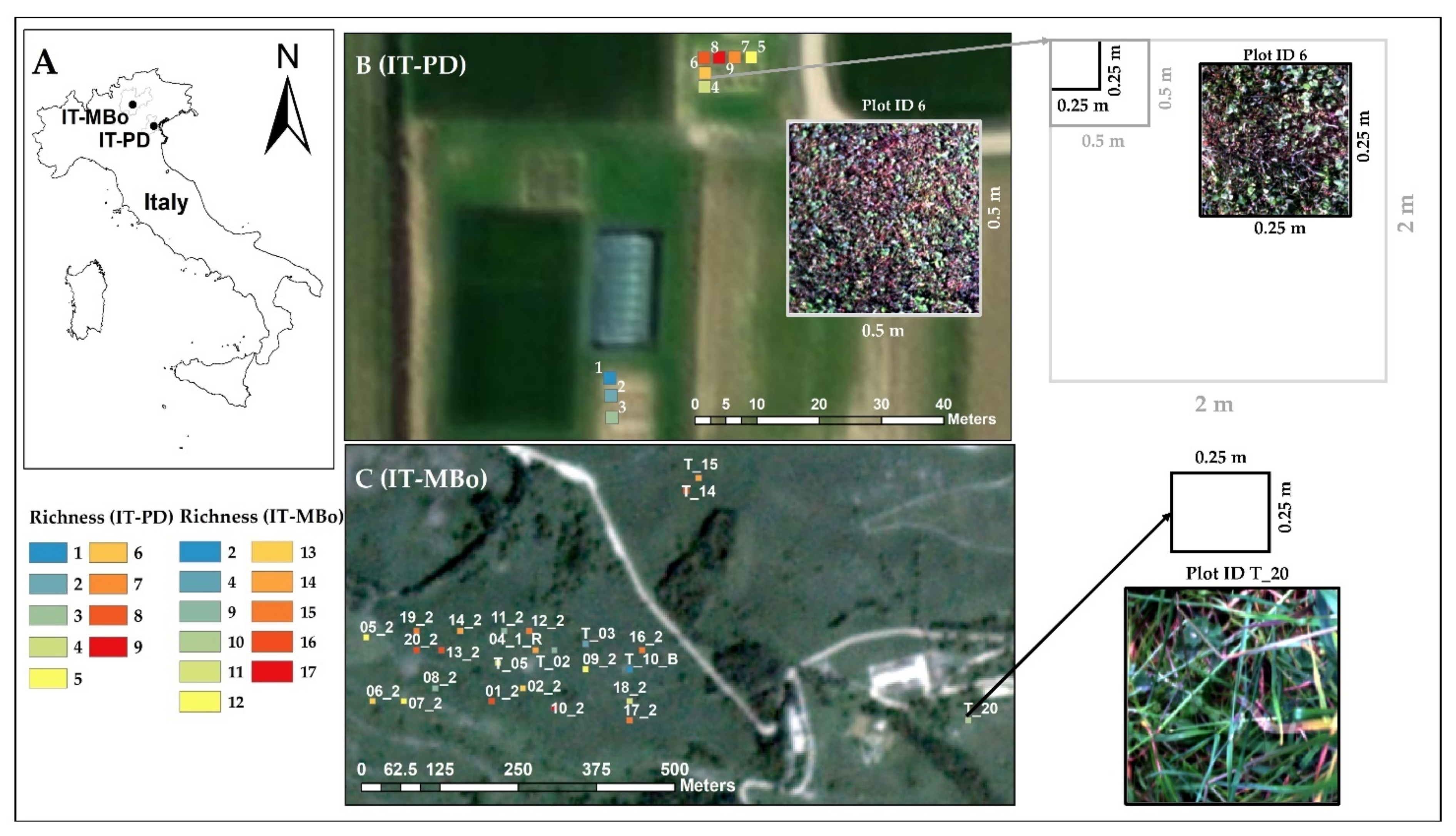
The dataset used in this study was collected at two grassland sites characterized by different structure, species composition, and origin (
Supplementary Materials,
Figure S1). The first site was a turf grassland (
Figure 1) located on the Experimental Farm of the University of Padova, in Legnaro, Italy (45°21′ N, 11°58′ E; 6 m a.s.al., IT-PD), where plots of varying species richness (ranging from 1 to 9) were established in September 2018 by seeding. The established plots were arranged in a square (2 × 2 m) design and were managed by removing weeds and mowed with a rotary mower machine at approximately 4.7 mm every other week. Subplots with dimensions of 0.25 × 0.25 m and 0.5 × 0.5 m were chosen within the 2 × 2 m square plots for the spectral and biodiversity analysis. The species composition of the investigated plots at IT-PD is summarized in
Table S1 in
Supplementary Materials.
The second site was a permanent semi-natural grassland (
Figure 1) situated in the Italian subalpine vegetation belt at Viote del Monte Bondone, Trentino province, Italy (46°00′ N, 11°01′ E; 1480–1550 m a.s.al., IT-MBo). The grassland area lies on a plateau, and it is managed extensively as a meadow with low mineral fertilization. It is cut once a year around mid-July at the green biomass peak time, and it is characterized by very high plant diversity [
42]. Several different vegetation types can be found in the area with extremely varying canopy structure and biomass [
43,
44]. The
Sieverso-Nardetum strictae association covers a high portion of the plateau characterized by short canopies. The
Scorzonero Aristatae-Agrostidetum tenuis association canopy is generally taller, and it grows on calcareous soils. The latter association includes more productive species, and it can be found in the most fertile and well-exposed areas of the plateau [
43]. The species composition of the 25 investigated plots (0.25 × 0.25 m) of the IT-MBo plateau is summarized in
Table S2 in
Supplementary Materials.
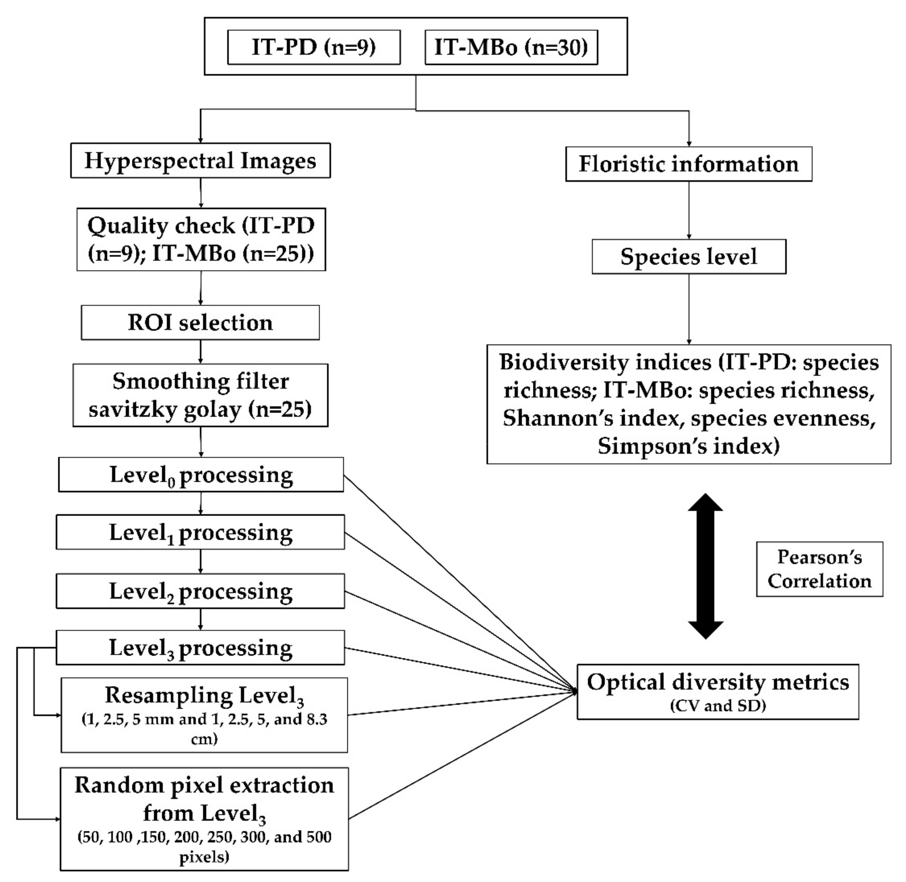
The methodological flowchart of the study is shown in
Figure 2. In the following sections, each step is described in detail.
2.2. Biodiversity
To collect the floristic information, vegetation surveys were carried out by a trained person within the study areas. At the IT-PD site, the species number was counted after identification of all species within the ROI (0.25 × 0.25 m and 0.5 × 0.5 m). At the IT-MBo site, the species composition was determined by listing all plant species within the ROI (0.25 × 0.25 m) and visually estimating their percent cover [
45]. Species percent cover information was used to calculate the following biodiversity indices: species richness (S), Shannon’s index (H’), Simpson’s index (D), and species evenness (J, calculated as Pielou’s index). The details regarding the biodiversity indices are reported in
Table 2. All biodiversity indices were calculated using the ‘vegan’ R package [
46].
2.3. Spectral Data Acquisition
At the IT-PD site, the hyperspectral data of the nine plots were collected in the summer of 2019 by means of a SPECIM IQ hyperspectral camera (SPECIM Ltd., Finland). The spatial sampling of the camera is 512 pixels per line and the spectral resolution is 7 nm, with 204 bands across the VIS (397 nm–700 nm) and NIR (700 nm–1003 nm) spectral range. The hyperspectral camera was mounted on a tripod and two nadir images were collected at approximately 1 and 2 m from the ground (with an image footprint of approximately 0.55 × 0.55 m and 1.1 × 1.1 m, respectively). The images were acquired using the simultaneous mode (the white reference panel was recorded simultaneously with the targeted vegetation). For both study sites, the spectral data were acquired between 11:00 and 14:00 local time under clear sky conditions. To record the images, an integration time of 1 ms was used, which provided a weak signal, but ensured non-saturated images. The SPECIM IQ did not allow the acquisition of non-saturated images with higher integration time under clear sky conditions. The ROIs (0.25 × 0.25 m and 0.5 × 0.5 m) of the IT-PD images were extracted and used for post-processing and spectral diversity metrics calculations. The distance from the canopy was approximately 1 m for IT-PD and 0.7 m for IT-MBo site. Although the distance between the canopy and the camera was kept as constant as possible, the number of pixels within the ROIs was not exactly the same due to slight variation in canopy height. In the IT-PD plots, the average number of pixels per ROI was 64,260 pixels, with an average pixel size of 1 mm (pixel size: min, 0.95 mm and max, 1.02 mm) and 10,8240 pixels with an average pixel size of 1.5 mm (pixel size: min. 1.48 mm and max. 1.56 mm) within the ROIs of 0.25 × 0.25 m and 0.5 × 0.5 m, respectively.
At the IT-MBo site, we selected 30 randomly distributed plots with species richness ranging from 2 to 17. In the summer of 2018, at the biomass peak time, we collected canopy level spectral data using the same SPECIM IQ camera. The canopy height at IT-MBo was not consistent between the plots (varied from 0.3 to 1.2 m); therefore, the hyperspectral images were collected approximately 0.7 m from the canopy level to capture a squared footprint of approximately 0.55 × 0.55 m. A 0.25 × 0.25 m frame was placed within each image footprint to define the ROIs used for post-processing and spectral diversity metrics calculations. The average number of pixels within the IT-MBo ROIs was 84,100 with an average pixel size of 0.9 mm (pixel size: min, 0.70 mm and max, 1.48 mm). All the 30 plots images were visually evaluated to remove any blurred (because of moving leaves due to windy conditions) and out of focus images. Finally, 5 plots were discarded after the quality check of the hyperspectral images and 25 plots were kept for further analysis.
2.4. Pre- and Post-Processing
ROIs were extracted from the image using the ENVI (version 4.8) software. For further processing, we used the open-source statistical software R [
48]. The pre- and post-processing of the hyperspectral data were categorized into four processing levels. In Level
0, corresponding to processing of the raw spectral data, the bands 397–411 and 930–1003 nm were removed to avoid the use of noisy data which were detected in these spectral regions [
10]. To further reduce the noise in the spectral signature, a Savitzky–Golay smoothing filter [
49] was applied using a 25-band window width.
The brightness of the spectra may be affected by heterogeneous illumination, leaf volume, or subpixel shade [
50]. For Level
1 processing, we applied brightness normalization [
50] to all the images and then calculated the optical diversity metrics from the brightness normalized images.
For Level
2 processing, we applied specific filters to remove bright pixels from the images, alongside pixels containing flowers, shadows, and soil background, as they are not linked to plant biodiversity. We used the red band (680 nm) to remove shadowed pixels [
51], and the thresholds were defined by visual interpretation. Pixels with red band reflectance below the first quartile were found to be suitable for obtaining a reliable separation between shaded and sunlit pixels for the investigated plots. To filter the flower pixels, we used the red-green normalized difference vegetation index (NDVIrg) based on the red and green bands (640 and 551 nm, respectively). Pixels with an NDVIrg value higher or equal to the visually selected threshold of 0.1 were excluded [
52]. Furthermore, to remove the bright pixels in the images due to hot spots at the leaf level, we used the NIR band (865 nm) and selected a threshold value (>third quartile) to filter out the over-illuminated pixels. To remove dead leaves pixels, we used a normalized difference vegetation index (NDVI) mask (≤0.7) for all of the images. For Level
2 processing, about 46% for IT-PD and 54% for IT-MBo of the pixels from the total number of pixels within the ROIs were classified as shadows, flowers, dead leaves, and bright pixels and were filtered out.
To normalize the spectral features and reduce noise, spectral vegetation indices are commonly used to remotely evaluate vegetation covers both quantitatively and qualitatively [
53]. In some cases, transformed (continuum-removed—CR) spectra is used to normalize reflectance data [
24]. To further improve the quality of the images for Level
3 processing, we, therefore, calculated the CR spectra from the Level
2-processed data.
2.5. Calculation of Optical Diversity Metrics
As an indicator of the optical diversity of each plot, we used two spectral diversity metrics: the CV (i.e., ratio of the standard deviation to the mean, [
13,
41]) and the SD calculated as the average across the spectrum [
13] from the Level
0-processed data using the following equations:
where
represents the reflectance value at wavelength
and std (
) and mean (
) indicate the standard deviation and mean value of the reflectance at wavelength
, respectively. The average CV and SD were also calculated considering different spectral regions (408–499 nm, 500–589 nm, 590–674 nm, 675–754 nm, and 755–930 nm) as in Aneece et al. [
24] from the Level
0-processed data. We also calculated the CV and SD for each spectral band using Equations (3) and (4) from the original images and for each of the post-processing levels (Level
0 processing, Level
1 processing, Level
2 processing, and Level
3 processing) described in
Section 2.4:
where
represents the reflectance value at the wavelength
and std (
) and mean (
) indicate the standard deviation and mean value of the reflectance at the wavelength
, respectively. The CV and SD calculated from the fully transformed Level
3 reflectance (brightness normalized, filtered, and CR) are shown in
Figure 3 (IT-PD CV: E and IT-PD SD: F) and
Figure 4 (IT-MBo CV: E and IT-MBo SD: F).
The effects of pixel resolution and random pixel extraction on the relationship between optical diversity and biodiversity indices were tested at both sites. To study the impact of spatial resolution, the original data were resampled using the nearest neighbor algorithm to different spatial resolutions (1 mm, 2.5 mm, 5 mm, 1 cm, 2.5 cm, 5 cm, and 8.3 cm), processed with Level3 processing, and then the obtained pixels (approximately 54% of the pixels for IT-PD and 46% for IT-MBo) were used to calculate the optical diversity metrics at each resolution. Finally, to evaluate the sample size effects on the relationships between optical diversity and biodiversity indices, a varying number of pixels (50, 100, 150, 250, 300, and 500) were randomly extracted from the Level3-processed data. Pixel random extraction was re-iterated 10 times and the optical diversity metrics were calculated at each extraction, and the 10 R values of the correlations between biodiversity and optical diversity metrics were averaged.
2.6. Statistical Analysis
The Pearson correlation coefficient (R) and the corresponding
p values between the optical diversity metrics (CV and SD) and the biodiversity indices (species richness, Shannon’s index, Simpson’s index, and species evenness) of the surveyed plots were calculated with the “cor.test” function in the “stats” package separately for the two grassland sites. Calculations were done for both the original and transformed reflectance data. Normality of the data and residuals of the correlation between the best correlated optical diversity metrics and the field-measured species richness was checked with a Shapiro–Wilk test using the “shapiro.test” function in the “stats” package. The analyses were performed with the statistical software R (version 3.6.1) [
48].
3. Results
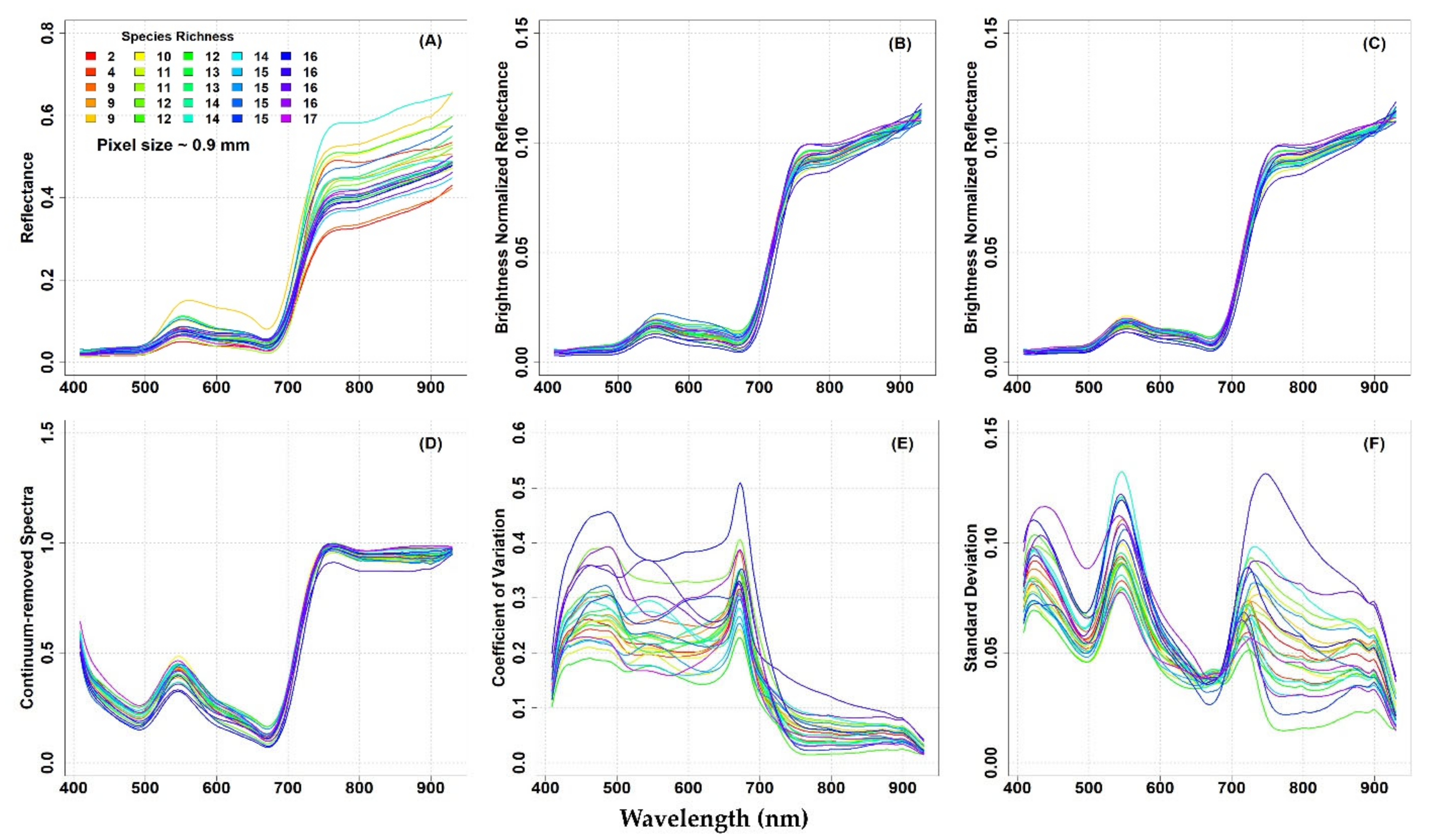
In
Figure 3 and
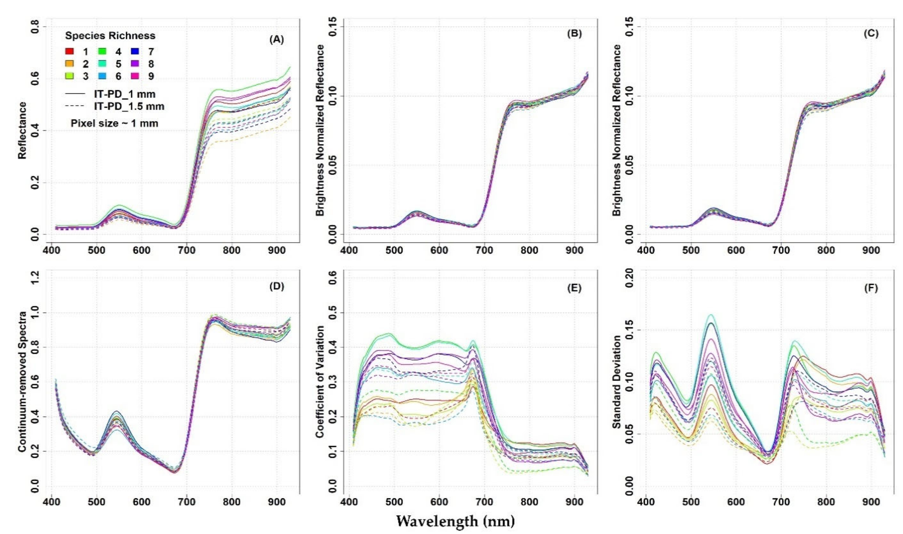
Figure 4, the mean original reflectance (panel A), mean transformed reflectance (panels B–D), and the spectral diversity metrics (CV and SD, panels E and F, respectively) from each plot are presented with respect to the plot species richness at both study sites.
The original mean reflectance values of the different plots showed some variability, especially in the NIR domain, at both study sites (
Figure 3A and
Figure 4A). Reflectance values and spectral variability among the plots was reduced when brightness normalization was applied to the hyperspectral image (
Figure 3B and
Figure 4B). Additionally, the variability was slightly reduced when a filter was used to remove flowers, shadows, and bright pixels from the images C and
Figure 4C). The CR spectra calculated from the brightness normalized and filtered images also showed low variability in the spectra, at both study sites (
Figure 3D and
Figure 4D).
At the IT-PD site, the mean original reflectance obtained from the 1 mm pixel size data (solid line,
Figure 3A) was higher compared to the mean reflectance from the 1.5 mm pixel size data (dashed line,
Figure 3A). There was not much difference observed between the mean spectra from the two different spatial resolutions (1 and 1.5 mm) at different processing stages (
Figure 3B–D). In general, the reflectance increased with the increase of species richness from 1 to 4 and then it started to decrease (
Figure 3A). On the other hand, at the IT-MBo, a clear link of the reflectance values with species richness was not noted (
Figure 4A).
The optical diversity measured by the CV from the Level
3-processed data showed that the spectral variability in the reflectance within plots was particularly high in the VIS part of the spectrum, while the variability in the NIR spectral region was low (
Figure 3E). In general, the highest CV values were observed in the plots where four species were observed, while the lowest CV values in the plots with three species (
Figure 3E). Therefore, no manifest association with plant biodiversity was observed. The SD showed three peaks in the blue, green, and red-edge spectral domains, and the lowest SD was detected around 680 nm (
Figure 3F).
The lack of relationship between the spectral diversity across the spectrum (CV and SD) and species richness was particularly pronounced at the IT-MBo site (
Figure 4). Similarly to the IT-PD site, the CV at the IT-MBo site showed that variability was observed mainly in the VIS part of the spectrum, while the NIR spectral region was characterized by low variability (
Figure 4E). The SD at IT-MBo showed three peaks across the spectrum (
Figure 4F). As in the IT-PD dataset, the highest values of SD were found around the blue, green, and red-edge part of the spectrum, while the lowest SD was detected around 680 nm at the IT-MBo site (
Figure 4F).
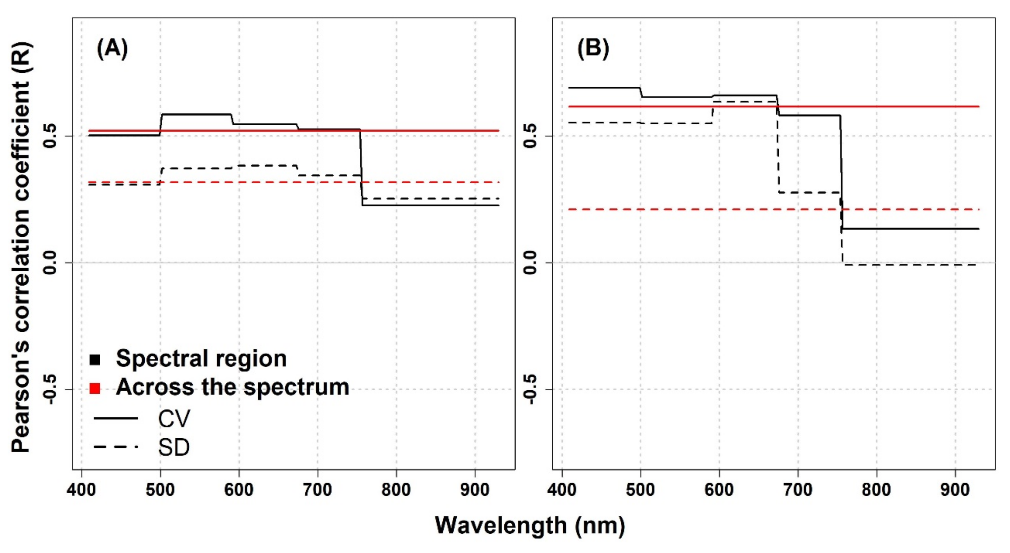
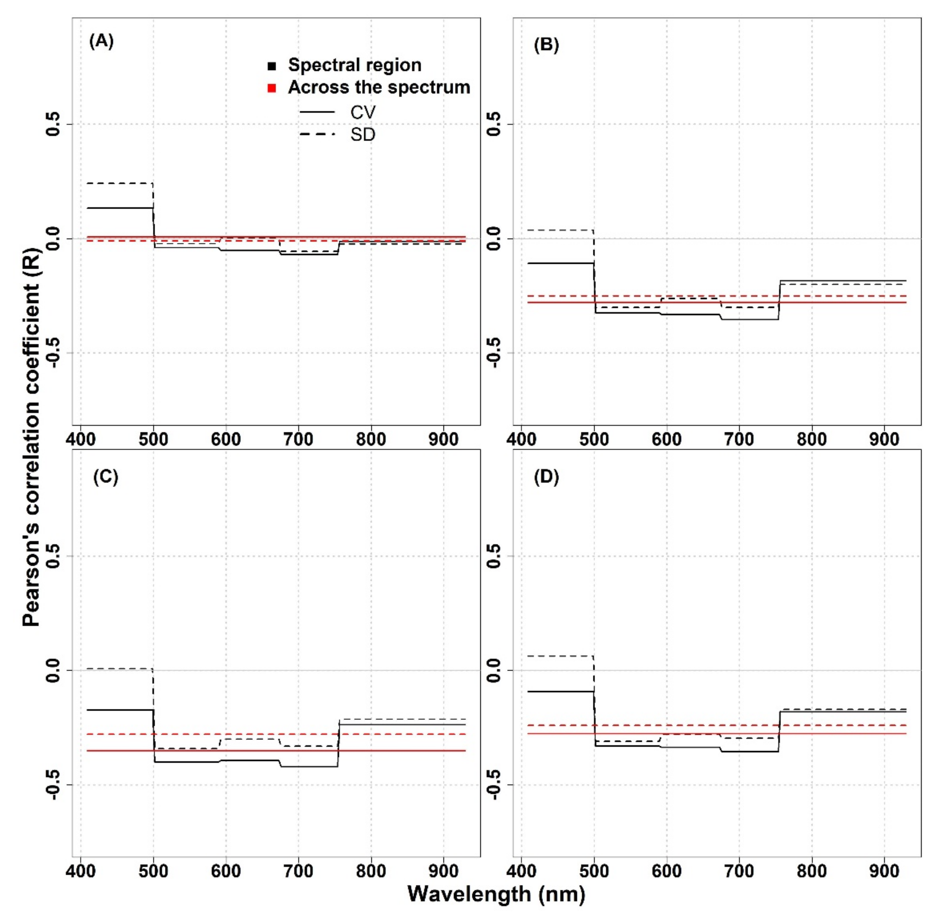
In this study, the performance of spectral diversity to estimate plant diversity was not consistent across the spatial scale, over different grassland ecosystems, and across different spectral regions. For the IT-PD site, the Pearson correlation analysis revealed positive correlations between optical diversity metrics (calculated from the Level
0 data and averaged across the spectrum) and species diversity except for the SD metric calculated from 1.5 mm pixel size data, which showed almost no correlation in the NIR part of the spectrum (
Appendix A,
Figure A1). For both datasets, the CV in different spectral regions showed higher R values compared to the SD metric in the VIS and red-edge part of the spectrum. On the other hand, in the NIR spectral region, both metrics showed weak correlations (1 mm: CV: R = 0.23,
p = 0.56, SD: R = 0.25,
p = 0.51; 1.5 mm: CV: R = 0.13,
p = 0.73, SD: R = −0.01,
p = 0.98). At the IT-PD site, generally weak correlations were observed between the CV calculated across the spectrum and species richness (1 mm: R = 0.52,
p = 0.15; 1.5 mm: R = 0.62,
p = 0.08), while the SD metric showed lower R values (1 mm: R = 0.31,
p = 0.41; 1.5 mm: R = 0.21,
p = 0.59) for both datasets. For the IT-MBo site, the spectral diversity metrics showed contrasting results with pervious work [
13,
24], highlighting a weak correlation between optical diversity and biodiversity indices. The correlations obtained between optical diversity metrics calculated from the Level
0 data averaged across the spectral regions and within different spectral regions showed almost no correlation with species richness, although a weak positive correlation for CV and SD averaged in the 408–499 nm spectral region was recorded (
Appendix A,
Figure A2, panel A). For other biodiversity indices (Shannon’s index, species evenness, and Simpson’s index) both optical diversity metrics (calculated from the Level
0-processed data) mostly showed an inverse correlation both when the CV and SD were averaged within different spectral regions and when it was averaged across the VIS-NIR spectral region (
Appendix A,
Figure A2, panels B,D).
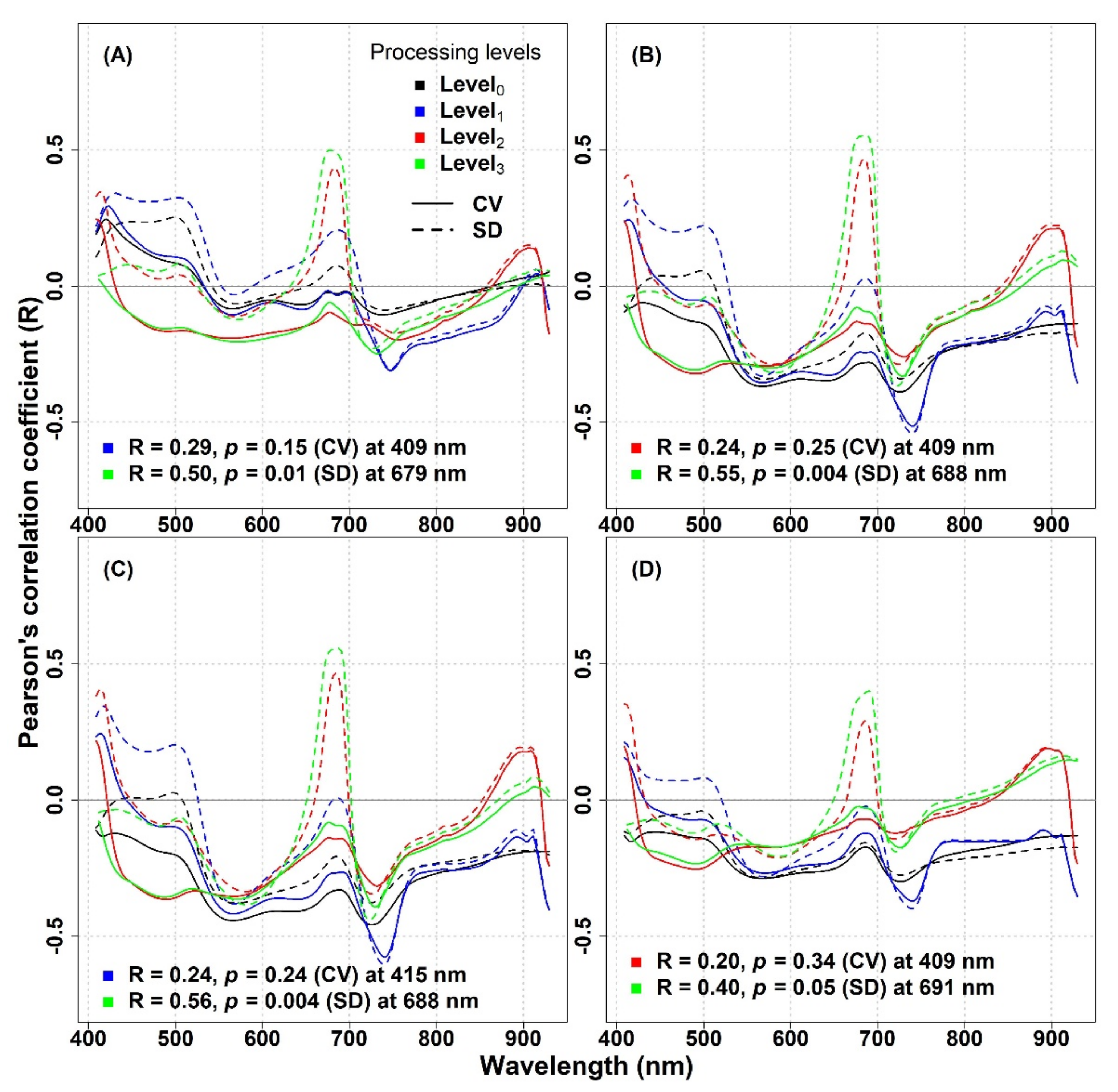
In a further step, to check the impact of image processing on the metrics performance, we calculated the CV and the SD for each spectral band from both untransformed (Level
0) and transformed (Level
1, Level
2, and Level
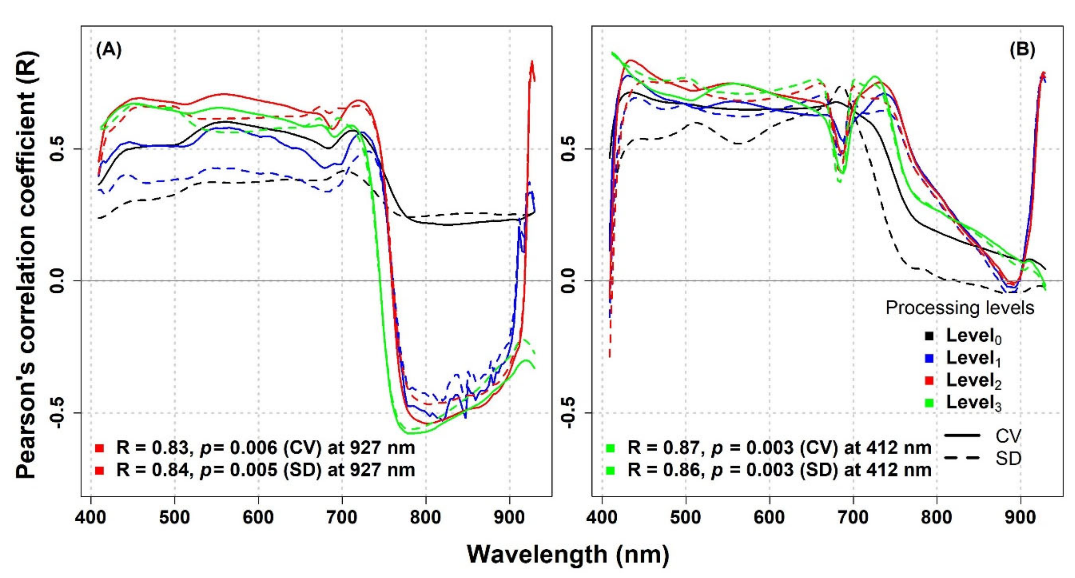
3) reflectance. We examined the correlations across the spectrum between species richness and both the CV and SD optical diversity metrics and we found high R values for both spatial scales: up to R = 0.83 (CV) and R = 0.84 (SD) and R = 0.87 (CV) and R = 0.86 (SD) for 1 and 1.5 mm pixel size, respectively (
Figure 5). We observed that the CV and SD calculated from transformed reflectance showed, in general, higher R values compared to untransformed reflectance. For the 1 mm pixel size image, the correlations between species richness and the CV and SD metrics calculated from the transformed reflectance were mostly positive in the VIS and negative in the NIR (
Figure 5). The maximum R values and their respective wavelengths for both datasets (1 mm and 1.5 mm) and various processing levels are reported in
Table S3.
At the IT-MBo site, the shape of the R values curve was very different compared to the IT-PD site (
Figure 6). Additionally, lower R values were occurring across the spectrum, with a small spike in the wavelengths around 680 nm for the SD calculated from Level
2 and Level
3 transformed reflectance. Similar trends were noted for R curves for all the investigated biodiversity indices (
Figure 6A–D). The maximum R values and their respective wavelengths and various processing levels at IT-MBo are reported in
Table S4.
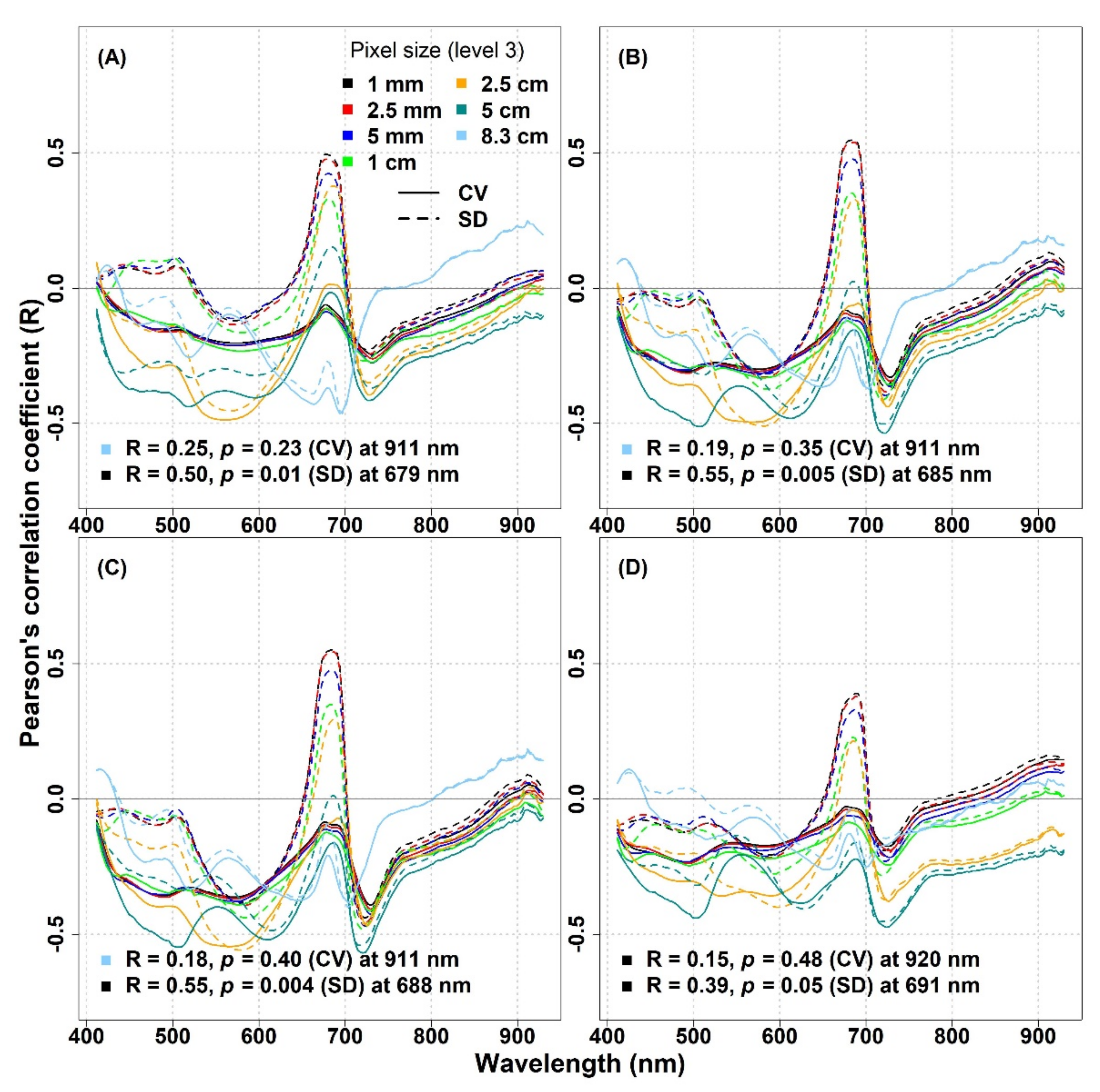
3.1. The Impact of Spatial Resolution on the Spectral Diversity–Biodiversity Relationships
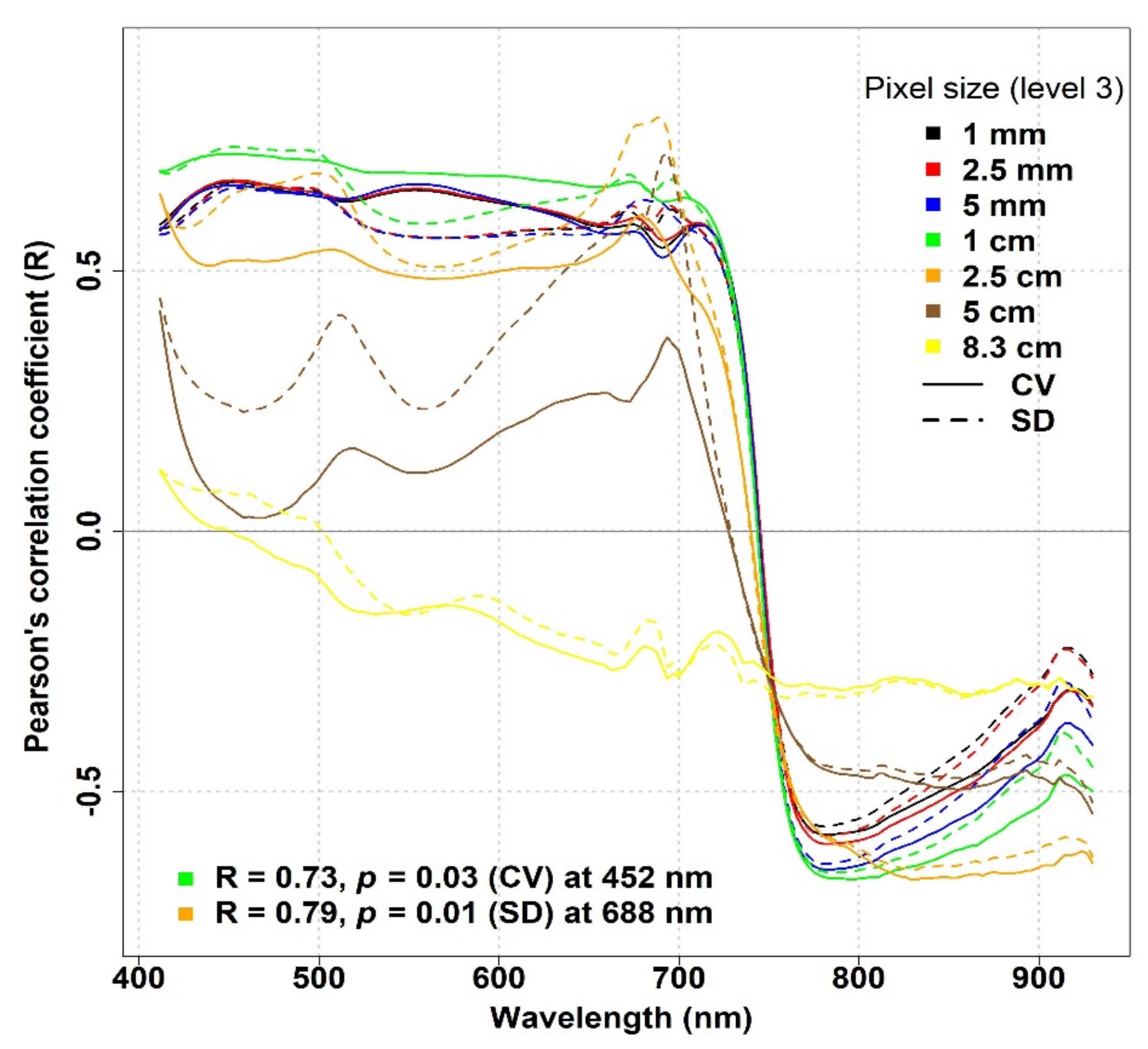
To study the scale effects, we investigated the relationships between optical diversity and biodiversity metrics at decreasing spatial resolutions (1 mm, 2.5 mm, 5 mm, 1 cm, 2.5 cm, 5 cm, and 8.3 cm) by resampling the original spectral data (
Figure 7). For the IT-PD site, in the VIS part of the spectrum a strong relationship between optical diversity metrics and species richness with an R value (R > 0.5) was recorded when pixel size was reduced up to 1 cm, while with a larger pixel size (>2.5 cm), the R values started to decrease, reaching a value of −0.15 when the pixel size increased up to 8.3 cm (
Figure 7). In the NIR part of the spectrum, a strong inverse correlation was obtained when the CV and the SD were calculated from 1 cm resampled data. The strength of the inverse correlation started to weaken when pixel size increased and the weakest correlation was noted with 8.3 cm pixel size data (R = −0.3). The maximum R values and their respective wavelengths across different spatial resolutions for the IT-PD site are summarized in
Table S5.
In
Figure 8, we considered the effect of pixel downsampling at the IT-MBo site. A clear difference in R values was observed between the two optical diversity metrics: around 680 nm, the SD showed a stronger correlation compared to the CV when the spatial resolution was reduced up to 5 cm, while for 8.3 cm, both metrics showed a weak inverse correlation with biodiversity indices around the same wavelengths. For the SD metric, the effect of pixel downsampling was noticeable when the pixel size went beyond 2.5 mm, as the maximum R value around 680 nm dropped from 0.48 to 0.12, 0.55 to 0.02, 0.54 to 0.01, and 0.39 to −0.16 for the species richness, Shannon’s index, species evenness, and Simpson’s index, respectively. In general, a similar pattern of R values was observed for all biodiversity indices, where the CV mostly showed an inverse correlation particularly around 550 nm, and the strength of the correlation increased with increasing pixel sizes up to 2.5 cm. On the other hand, for lower spatial resolutions (>2.5 cm), the strength of the correlation weakened, and for 8.3 cm, the weakest correlation was observed at the same wavelength. Similarly, at RE spectral bands (around 720 nm), the effect of decreasing spatial resolution could be noticed as the inverse correlation became stronger at increasing pixel sizes up to 5 cm.
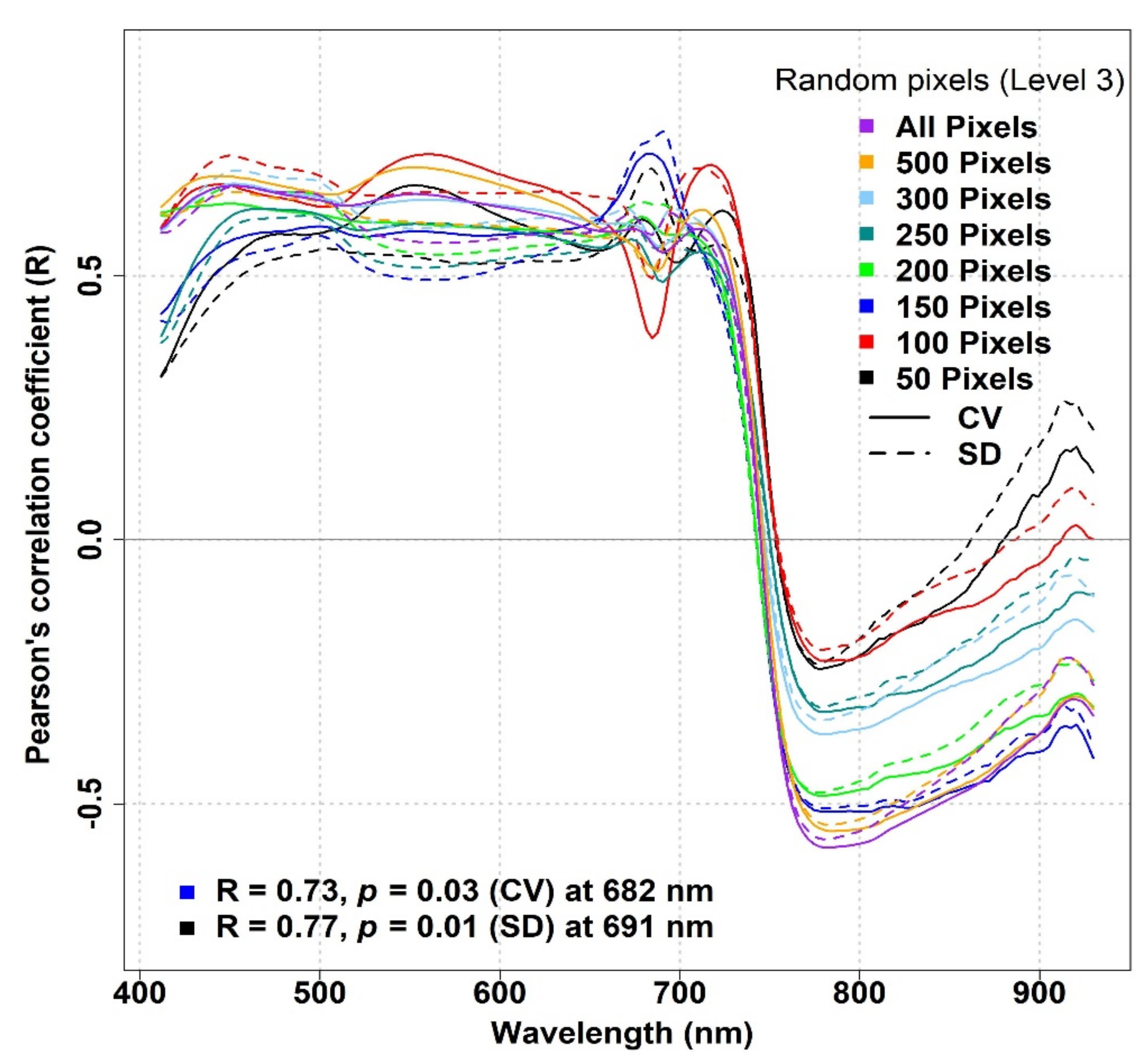
3.2. The Impact of Pixel Subsampling on the Spectral Diversity–Biodiversity Relationships
In
Figure 9, we present the results achieved by using the subsampling approach presented by Schweiger et al. [
15] to calculate the optical diversity. For the IT-PD plots, subsampling by random pixel extraction generally did not cause any major changes in the R patterns across the spectrum, except for the NIR region, in which subsampling based on 50, 100, 250, and 300 pixels resulted in a noticeable reduction in the R values (
Figure 9). Nevertheless, positive R values were observed in the VIS part of the spectrum, while mostly negative R values were observed in the NIR spectral bands.
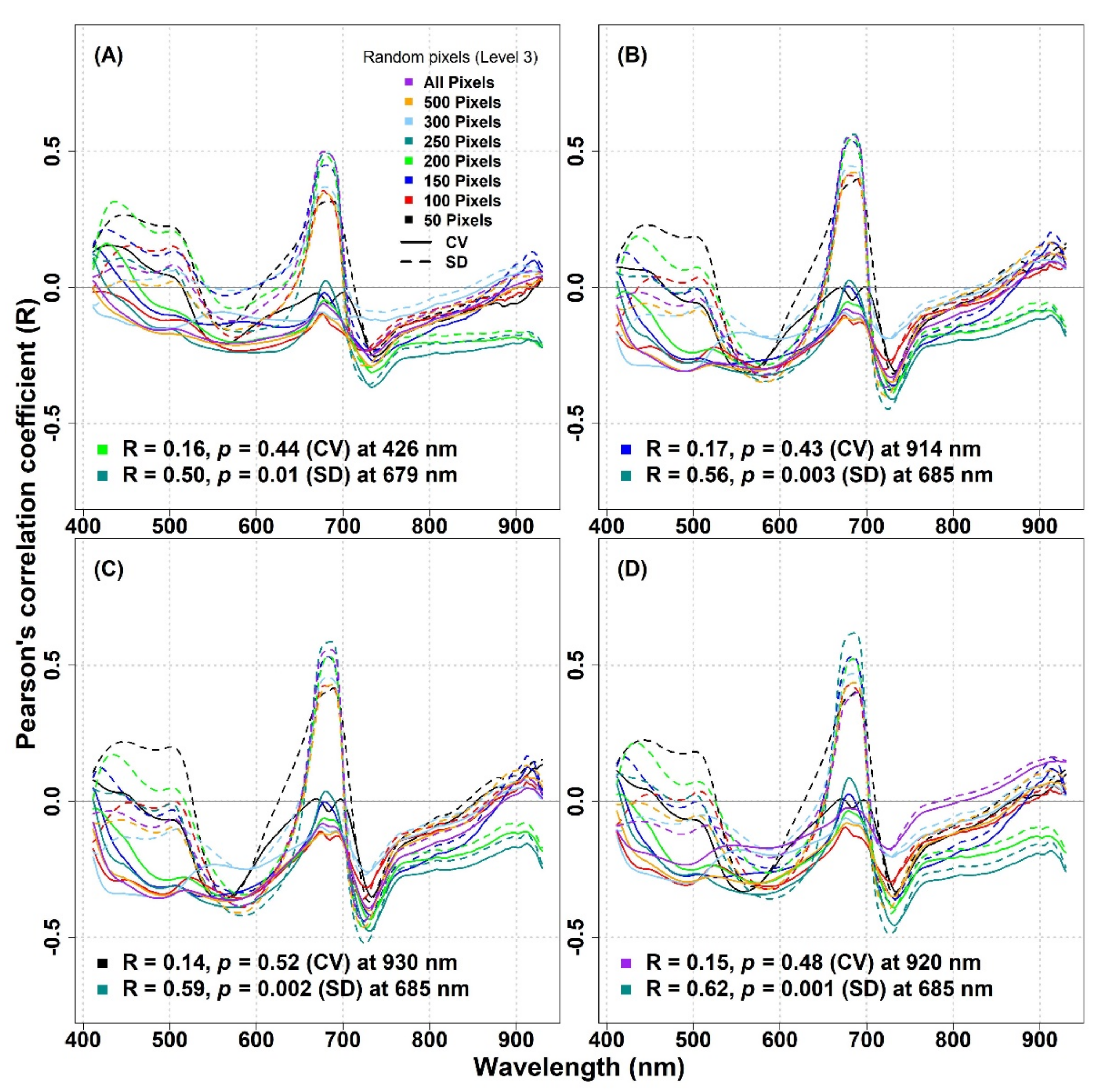
Similarly, for the IT-MBo site, there were generally no considerable improvements in the correlation coefficient between the optical diversity metrics calculated using randomly extracted subsample pixels and biodiversity indices compared to the results found between the same metrics when considering all pixels (
Figure 10). In general, the SD metric showed stronger relationships with biodiversity indices compared to the CV metric. The highest R value (R ≥ 0.5) was observed around 680 nm when 250 pixels were used to calculate the SD for all biodiversity indices, while for the CV around the same wavelength, very low R values (R ≤ 0.09) were obtained (
Figure 10A–D). For the IT-MBo site, the strongest relationship was observed between the Simpson’s index and the SD metric calculated with 250 pixels at 685 nm (R = 0.62,
p = 0.001,
Figure 10D).
4. Discussion
Similarly to other authors [
13,
14,
24], our study found a significant relationship between spectral diversity (expressed as CV and SD) and species diversity in the lower-diversity artificial grassland site. However, the data acquired at the semi-natural subalpine grassland at IT-MBo with the same methodology and analyzed with the same approach provided much weaker correlations. Such results may be due to the very high level of biodiversity (up to 17 species in a 0.25 × 0.25 m plot) and to the rather complex structure of the IT-MBo grasslands [
44] compared to the low-diversity turf canopy at the IT-PD site. Our main findings questioned the applicability of the optical diversity method to estimate biodiversity in highly diverse grasslands, such as the ones at the IT-MBo site. Despite the fact that we used several different processing techniques to enhance the optical diversity signal, for the subalpine grassland site of IT-MBo, we were not able to match the performance of optical-based methods to estimate the biodiversity reported in other studies [
13,
14,
24]. In Aneece et al. [
24], an artificial ecosystem (with max. 5 species/m
2) was investigated, and the maximum R
2 value of the correlation between the optical diversity and α-diversity was 0.43. Wang et al. [
13] carried out on an artificial grassland (max. 16 species/m
2), in which the maximum R
2 value reached 0.58, while in the study of Peng et al. [
14], which focused on natural grasslands (with a maximum species richness of 12 in a 0.8 m diameter plot), the maximum R
2 value reached 0.40.
In our study, when optical diversity metrics were averaged across different spectral regions as in Aneece et al. [
24] and across the spectrum as in Wang et al. [
13], we found contradictory results at the two sites. At the IT-PD site, a positive correlation between optical diversity metrics and biodiversity indices was mostly observed, while at the IT-MBo site, the correlation was mostly negative (IT-PD and IT-MBo;
Appendix A,
Figure A1, panels A, B and
Figure A2, panels A–D, respectively). When the CV and the SD were calculated for each spectral band on a separate basis, the R reached much higher values: 0.84 (SD metric at 927 nm) and 0.87 (CV metric at 412 nm) in the artificial turfgrass (maximum number of species was 9 in a 0.25 × 0.25 m and 0.5 × 0.5 m area). The maximum R value in the species-rich subalpine grassland was only 0.56 for the SD metric at 688 nm (maximum number of species was 17 in a 0.25 × 0.25 m area,
Figure 6, panel C). Considering these results, we may conclude that the optical diversity approach appears more suitable for lower-diversity or artificial systems, and its application may be more challenging in highly diverse grasslands.
The applicability of the methods to estimate species diversity using hyperspectral data was also questioned by other authors [
28,
31]. In these studies, the relationships between species diversity and optical diversity metrics were not consistent across plant communities. Lucas and Carter [
31] evaluated the prediction of species diversity (species richness) in Horn Island, Mississippi by using ground transect data and remotely sensed data. However, they failed to find a significant relationship between spectral diversity metrics and species richness, which may be due to the fact that their study considered highly diverse habitat types. Gholizadeh et al. [
28] investigated the SVH-based approaches to access the α-diversity in Cedar Creek Ecosystem Science Reserve in Central Minnesota, USA and highlighted the effect of soil background on the performance of optical diversity metrics. The authors achieved significant correlations between spectral diversity metrics and the species richness when they applied an NDVI filter to remove the soil background from the hyperspectral image. In our study, however, the impact of soil was minimal, as the fractional cover of the vast majority of the plots was 100% (it was lower than 100% in only eight plots, but always higher than 99.5%). Wang et al. [
13] provided significant and detailed insights on the possible factors affecting the optical diversity and biodiversity relationships, highlighting the fact that canopy structure effects can determine substantial illumination and scattering differences and both leaf traits and canopy structure strongly influence optical diversity metrics. As a consequence of the fact that canopy structure can influence the optical diversity and modify the optical diversity–plant diversity relationships, we can expect that in heterogeneous grasslands characterized by complex structural patterns and by a very high number of species, biodiversity estimations based on optical diversity are not always reliable.
In this work, we adopted a range of techniques to fully disentangle the optical diversity due to plant diversity from the optical diversity due to illumination artifacts, or due to the presence of pixels of non-photosynthetic material, such as dead material or flowers. The results of this paper highlight the impact of image processing techniques on the relationships between optical data and grassland diversity. The developed processing flow proved, in general, to slightly improve the remote estimations of plant diversity, by limiting the influence of the factors determining optical diversity but not related to plant diversity. As shown by other authors, spectral diversity is affected by canopy non-photosynthetic elements, such as flowers and, dead material, as well as by shaded pixels, overexposed pixels, and the soil background [
13,
14,
28,
36]. To normalize the effect of shadows, Feilhauer et al. [
50] proposed the brightness normalization approach to minimize the spectral differences between the sunlit and shaded areas. In the present study, we observed that after applying brightness normalization to the hyperspectral images, the reflectance variability in the NIR was strongly reduced. In our case, the performance of the models to estimate grassland biodiversity did not significantly improve compared to the original dataset when this transformation method was used alone. However, the filtering of flowers, shadows, and bright pixels and then the transformation of the reflectance to CR minimized the spectral differences, which were not linked to species diversity and improved the diversity estimations. Heumann et al. [
19] studied the impact that flowers have on spectral diversity and investigated how this may influence the applicability of the spectral diversity hypothesis. These authors reported that the inclusion of flower spectra increased the normalized root mean square error (nRMSE) by 30% for Shannon’s diversity index, because there would be more inherent spectral diversity for each given species due to the spectral response difference between leaves and flowers.
The optical diversity–plant diversity relationships appeared to be both ecosystem-dependent and scale-dependent. Spatial scale was shown to strongly affect the spectral diversity–biodiversity relationships. In the study of Wang et al. [
13], with decreasing spatial resolution, the variability in reflectance and, therefore, CV and SD decreased, and the optical detectability of biodiversity was reduced. In our study, however, the correlation between optical diversity metrics and species richness initially increased and was only reduced when the pixel size was beyond 2.5 cm in IT-PD, even if for most of the species the average leaf size was much lower than this value. For IT-MBo, the optimal pixel size (at 680 nm) was 1 mm. Conversely, according to Wang et al. [
13] the optimal pixel size to detect species diversity using spectral diversity should match the size of the objects within the sampling unit.
Another key finding of this paper concerns the impact of processing methods on the performance of the optical diversity approach. When we compared the performances of the CV and SD metrics, we demonstrated that Level
3 data generally showed higher correlations with biodiversity indices, and that the use of CR spectra generally improved the R values of the correlation between SD and species diversity. Similarly to Blanco-Sacristán et al. [
41], we found that the spectral bands in the red part of the spectrum (around 680 nm) showed to be best for estimating biodiversity in both grasslands. In our study, a random extraction of pixels did not improve our results as in Schweiger et al. [
15], who achieved successful results based on links between spectral, functional, and phylogenetic diversity.
Man-made grasslands, obtained by sowing, are simplified ecosystems which may not be representative of the complexity of natural field ecological conditions, where leaf and canopy traits can contribute to optical diversity in several ways, adding complexity to the optical and plant diversity relationships in natural grasslands [
54]. This can explain the poor performance of the optical sampling methods in complex grassland canopies. In this respect, Wang et al. [
40], adopting a modeling approach, observed that grassland biodiversity estimations are strongly affected by species intra-variations, which can be relevant even when caused by a single species. In natural grasslands located in heterogeneous landscapes such as the environment of the Alps, where (i) different associations and sub-associations can be found within a few meters distance, and transition zones are very frequent, (ii) geomorphology, soil characteristics and origin, and grassland vertical structure profile can strongly vary on the spatial basis, and (iii) the number of species is particularly high, estimating grassland α-diversity using optical methods can be extremely challenging. From an ecological point of view, Grace et al. [
39] highlighted the limits of manipulation experiments and the need for more analyses focused on mature natural ecosystems. In this regard, these authors stated that the ecological mechanisms cannot be extrapolated from studies of synthesized assemblages to mature natural ecosystems. Analogously, the optical diversity approach—based on grassland functional diversity dynamics determining spectra variability—may not be always transferable to mature and very complex natural grassland ecosystems.
The VIS part of the spectrum (and in particular the red domain), characterized by a strong absorbance, showed to be one of the key spectral areas for biodiversity detection. This highlights the importance for further studies to investigate canopy biochemistry variability and its link with both biodiversity and optical diversity. To detect α-biodiversity using optical methods, we should be able to detect biochemistry content and its variability within the canopy. However, this may not be possible when grasslands with heterogeneous structure are observed. Previous studies on the IT-MBo grasslands [
44] determined how, due to structural complexity and heterogeneity, plant trait co-variation can strongly affect the ability to retrieve grassland traits using spectral data. More work is needed to determine how, in different grassland ecosystems, the optical dissimilarity of canopy spectra captures grassland functional differences and biochemical content variability (at the plot and at the spatial scale) determined by plant diversity. Additionally, further research will be able to clarify if in complex heterogeneous ecosystems, such as the grasslands of the Alps, the optical diversity approach can be adopted at the spatial scale to detect β-diversity. Such insights will provide more robust information on the mechanisms linking the optical diversity and the overall plant diversity.
5. Conclusions
Our study provided important observations on the performance of high spatial resolution imagery for grassland plant diversity estimations. The relationship between optical diversity and biodiversity proved to be ecosystem-dependent. The spectral diversity approach to estimate biodiversity showed a similar performance to previous studies when artificially established grasslands were observed. On the other hand, in the natural subalpine grasslands of IT-MBo, this approach did not achieve satisfactory results, even if specific processing techniques were adopted to disentangle the optical diversity due to plant diversity from the optical diversity related to shadows, flowers, and brown material. The SD metric calculated from the Level3 data in the red spectral domain (around 680 nm) showed the best optical diversity metric to estimate biodiversity in both study sites. The results of our study showed that the use of the optical diversity approach as a proxy of plant diversity has some limitations, particularly when high-biodiversity natural landscapes are observed.
Spectral variation drivers include not only species richness but other important factors, e.g., intra-specific optical, biophysical, and biochemical variability. Other important factors include, e.g., vegetation structure, shadows, and phenology. Several post-processing methods (including brightness normalization, filtering of shadowed and bright pixels, non-photosynthetic element pixels filtering, and continuum removal) were tested successfully, which generally improved the performance of the optical diversity models. On the other hand, the pixel subsampling approach was not shown to be effective in our study. Interesting insights were provided by the scale effect study, such as that the optimum pixel size (1 cm) for biodiversity estimations—at the turf grass site—was generally higher than expected, according to previous studies. However, more advanced post-processing image methods or the adoption of higher resolution imagery (pixel size < 1 mm, which was not tested in this study) may improve the performance of the optical diversity metrics to estimate biodiversity even in heterogeneous grassland ecosystems. More studies are needed to fully investigate the mechanisms at the basis of the optical diversity, to highlight the pigment content variability and α-diversity relationships in high biodiversity grasslands, and to provide novel insights on the reliability of β-diversity estimations at the spatial scale.


 ,
, 


