Open Data and Deep Semantic Segmentation for Automated Extraction of Building Footprints

Abstract

Advances in machine learning and computer vision, combined with increased access to unstructured data (e.g., images and text), have created an opportunity for automated extraction of building characteristics, cost-effectively, and at scale. These characteristics are relevant to a variety of urban and energy applications, yet are time consuming and costly to acquire with today’s manual methods. Several recent research studies have shown that in comparison to more traditional methods that are based on features engineering approach, an end-to-end learning approach based on deep learning algorithms significantly improved the accuracy of automatic building footprint extraction from remote sensing images. However, these studies used limited benchmark datasets that have been carefully curated and labeled. How the accuracy of these deep learning-based approach holds when using less curated training data has not received enough attention. The aim of this work is to leverage the openly available data to automatically generate a larger training dataset with more variability in term of regions and type of cities, which can be used to build more accurate deep learning models. In contrast to most benchmark datasets, the gathered data have not been manually curated. Thus, the training dataset is not perfectly clean in terms of remote sensing images exactly matching the ground truth building’s foot-print. A workflow that includes data pre-processing, deep learning semantic segmentation modeling, and results post-processing is introduced and applied to a dataset that include remote sensing images from 15 cities and five counties from various region of the USA, which include 8,607,677 buildings. The accuracy of the proposed approach was measured on an out of sample testing dataset corresponding to 364,000 buildings from three USA cities. The results favorably compared to those obtained from Microsoft’s recently released US building footprint dataset.

1. Introduction

Building footprint extraction can be used in several application areas such as population density estimation [1,2], urban planning and mapping, building energy modeling and analytics [3,4], and disaster management [5,6,7]. The use of high-resolution remote sensing images (i.e., satellite and aerial) have been increasingly explored to obtain building footprint information. While the identification of building geometry from this type of imagery is time consuming and costly to perform manually, automatic feature extraction methods hold great promise. Image semantic segmentation methods, which address the problem of assigning a categorical label (class) to each pixel of an image, is one of the most commonly studied approaches for automatic extraction of features from remote sensing images. Until recently, the semantic segmentation algorithms that have been employed to process remote sensing images were based on image feature engineering, which were often hand-crafted for each situation based on the category of object that was considered. However, due to the high variability of building footprint appearances, environmental characteristics such as surrounding vegetation and terrain conditions, as well as the impact of the type of sensor that has been used to collect the imagery (e.g., different resolution), methods based on hand-crafted features are difficult to design and have not produced accurate results.

The recent development of deep learning algorithms has considerably improved the ability to accurately extract information from images using machine learning (ML). These advances have triggered the interest of the remote sensing community in the adoption of this type of method to extract a variety of information from satellite and aerial imagery. More specifically, deep convolutional neural network semantic segmentation algorithms have revolutionized the computer vision field by providing an end-to-end learning approach that does not need feature engineering. Deep convolutional neural network algorithms learn different image features by building a hierarchy of data representation, which make this type of algorithm very efficient in processing complex real-world images such as remote sensing images. Thus, deep convolutional neural networks have been applied to several tasks in extracting information from satellite and aerial images such as road extraction [8,9], farm segmentation [10], building footprint segmentation [11,12,13,14] and building damage assessment [15,16]. These existing research studies have shown that the end-to-end learning approach based on deep learning algorithms significantly improved the accuracy of automatic building footprint extraction in comparison to more traditional methods that are based on the features engineering approach.

One of the biggest challenges of semantic segmentation is the availability of labeled training datasets. Most of the existing studies of building footprint extraction using deep convolutional neural networks employed benchmark datasets that have been manually labeled and curated [17,18]. However, these datasets are limited to a small number of U.S. cities, making it difficult to use them to develop a model that can be generalized to the entire U.S. territory, because of the high degree of variability in building shapes and US terrain topography. For instance, Maggiori et al. [13] include six US cities (i.e., Austin, TX; Chicago, IL; Kitsap county, WA; Bellingham, WA; San Francisco CA; Bloomington, IN) and there is just one city (i.e., Las Vegas, NV) in [17]. In addition, because of the costly manual labeling and curating process, the approach of manually creating training data is not a scalable solution, especially when a significantly high number of cities are considered. Openly available GIS data are another option that can be considered for automatically generating labeled training datasets.

OpenStreetMap (OSM) is currently the largest openly licensed database of geospatial data (i.e., GIS data). It is a global dataset that is a collaborative crowd-source product, supported by more than one million volunteers who have contributed to editing the database content. It includes different types of GIS information, such as road infrastructure and built environment, and it is used in many projects as an alternative to proprietary or authoritative data. While the crowd sourced nature of OSM has been a key to its success, the small number of volunteers with professional GIS experience has raised significant concerns about its accuracy. Several studies [19,20] have performed an assessment of OSM spatial accuracy and completeness of building footprints. However, because all these studies have focused their analysis on very limited geographical regions, it is not reliable enough to extrapolate a general conclusion regarding the quality of OSM in terms of building footprint. Touzani et al. [21] conducted, on a very limited sample of U.S. cities, a qualitative analysis of the OSM data accuracy and availability regarding building footprints. The authors noted that quality and availability vary significantly, and that this variability is highly correlated to whether or not the city’s authorities have made the building footprints openly available.

An increasing number of U.S. cities provide public building datasets through an easy to access open data web portal. Building footprints are provided by several cities (e.g., San Francisco, Washington D.C., Boston, Los Angeles, Chicago, New York) through such portals. The information is usually accessible via an application programming interface (API) or direct download, and it is available as a geographic information system (GIS) data file. In some cases, the height and some form of building ID is also provided. Using existing GIS tools, this type of dataset is generally easy to process. However, it is important to note that, although most of the city-provided data explored by the authors is regularly updated, some was found to be as old as 5 to 10 years, and therefore outdated.

The aim of this work is to use recent advances in deep semantic segmentation algorithms to extract building footprints from satellite images by leveraging the US openly available building footprint GIS data to automatically generate a large training dataset that, in comparison to the available benchmark datasets, has more variability in term of regions and type of city, which can be used to build more accurate deep learning models. However, in contrast to the previously mentioned benchmark datasets, in this study the generated training data are not manually curated. Thus, it is not perfectly clean in terms of the remote sensing images exactly matching the ground truth building’s foot-print. Another aim of this work is to explore how feasible it is to train an accurate model by using an approach that avoids the costly manual curation of the training dataset. The major contributions of this project are:

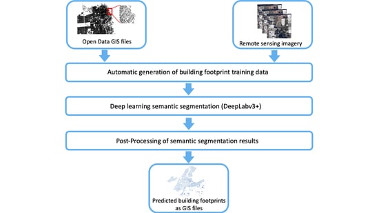
• Builds on previous research works, a framework for building feature extraction from satellite/aerial images is proposed. This uses a state-of-the-art deep semantic segmentation algorithm and a postprocessing step that convert predicted probability maps into GIS files that include building footprint polygons. It also utilizes openly available building foot-print GIS files to automatically generate labeled training data, which is a more scalable solution in comparison to the approaches that are based on the costly manual generation of training data.
• To the best of our knowledge this is the first attempt to explore the usage of such a high volume of training data (i.e., 15 cities and five counties from various regions of the USA, which include 8,607,677 buildings) that have been automatically generated using openly available public records and that have not been manually curated/de-noised.
• The proposed pipeline is tested and compared with another dataset of US building footprints that has been generate using a framework that also uses deep semantic segmentation and satellite images.

2. Datasets

2.1. Building Footprint GIS Open Data

In this work we collected building footprint GIS files from 15 cities–Austin, TX; Boston, MA; Chicago, IL; Denver, CO; Houston, TX; Indianapolis, IN; New York city, NY; Newark, NJ; Philadelphia, PA; San Francisco, CA; San Jose, CA; Seattle, WA; Tampa, FL; Virginia Beach, VA; Washington DC–and five counties–Allegheny County, PA; Fulton County, GA; Los Angeles County, CA; Miami Dade county, FL; Portland, OR. These cities and counties represented diverse regions spanning the geography of the United States. These GIS files were collected from the relevant authorities’ open data web portals (see

Table A1. Sources of used GIS files. The datasets were downloaded from these sources between March 2019 and June 2019.

City or County	Data Source
Austin, TX	https://data.austintexas.gov/
Boston, MA	https://data.boston.gov/
Chicago, IL	https://data.cityofchicago.org/
Denver, CO	https://www.denvergov.org/opendata/
Houston, TX	https://geo-harriscounty.opendata.arcgis.com/
Indianapolis, IN	https://data.indy.gov/
New York city, NY	https://opendata.cityofnewyork.us/
Newark, NJ	http://data.ci.newark.nj.us/
Philadelphia, PA	https://www.opendataphilly.org/
San Francisco, CA	https://datasf.org/
San Jose, CA	https://data.sanjoseca.gov/
Seattle, WA	https://data-seattlecitygis.opendata.arcgis.com/
Tampa, FL	https://city-tampa.opendata.arcgis.com/
Virginia Beach, VA	https://gis.data.vbgov.com/
Washington, DC	https://opendata.dc.gov/
Allegheny County, PA	http://www.wprdc.org/
Fulton County, GA	https://gisdata.fultoncountyga.gov/
Los Angeles county, CA	https://geohub.lacity.org/
Miami Dade county, FL	https://gis-mdc.opendata.arcgis.com/
Portland, OR	https://gis-pdx.opendata.arcgis.com/

in the Appendix A), and in total include 8,607,677 building foot-print polygons.

2.2. Remote Sensing Imagery

Several providers offer high resolution satellite or aerial images, either through an API or a direct download. However, one of the biggest challenges of using data that can be collected from these imagery companies is the licensing agreement, which can tightly limit the type of analysis that can be performed on these datasets and sharing of resulting derivate works (e.g., extracting a footprint from aerial images). Several providers allow free access to satellite and aerial imagery (e.g., Bing map, Google Maps), but they do not grant the user the right to download the images and to create derivative works.

Satellite/aerial orthoimages were collected from the satellite layer of Mapbox Maps [22]. Mapbox provides a high-resolution mix of satellite and aerial images that are a compilation of several commercial and open data sources. Mapbox allows researchers to freely use these images for non-commercial academic applications [23]. The Mapbox images are color-corrected and stored in raster format, which is a pixel-based data format “that efficiently represents continuous surfaces” [22]. The Mapbox images were retrieved using the Mapbox Raster Tiles API. For each GIS building footprint collected file, we created a list of tile coordinates that cover the specific region. These coordinates follow the Mapbox Raster Tiles API default format, which is the slippy maps standard [24] that defines each tile by the zoom level, which in turn defines the resolution and the tile coordinates. The zoom level that was selected for this work was 19. This level was chosen based on an empirical analysis that tested several zoom levels in the machine learning pipeline and compared the accuracy of the results on a very limited dataset. The total number of images (RGB) collected at zoom level 19 that cover geographical regions for which building footprints are available is 2,432,019, 512 by 512 pixels in size.

It is important to note that because the temporal resolution of the Mapbox imagery is not provided, the data used to train and evaluate the proposed approach will not be perfectly clean in terms of matching the ground truth building footprint to the satellite/aerial images. Thus, our work is based on noisier data than the previously cited research in the field. An example of this noise can be seen in Figure 1 images a and b; in the upper right corner it is clear that the footprint of the second building from the top is missing from the ground truth building footprint GIS files that were used to generate the “ground truth mask”. Having a discrepancy/noise between the truth and the training data is a more realistic scenario when the end-to-end deep learning approach are applied at scale, because manually curating millions of training images is not a trackable solution.

While this work was limited to Mapbox images, another potential source for gathering free aerial vertical imagery is cities’ open data portals. Cities such as New York City, Los Angeles, Portland, and Washington, D.C. regularly release high-resolution aerial imagery through their open data platforms.

2.3. Microsoft Building Footprint Dataset

Recently, Microsoft released building footprint GIS data covering the entire US territory. These data were generated from the satellite/aerial images available to Bing Maps. Similar to the methodology that is presented in this work, Microsoft’s building footprints were generated using a two-step approach comprising a deep learning semantic segmentation, followed by post processing. Unfortunately, there is no published information about which geographical regions were used to train the semantic segmentation model. Some information about the modeling and the post processing approach has been given in [25]. In this work we leveraged this data as a comparative benchmark.

3. Methodology

In this section we describe a workflow for building footprint extraction. All the code for the components of the proposed workflow is made openly available (i.e., AutoBFE (https://github.com/LBNL-ETA/AutoBFE, accessed on 16 March 2021)). This workflow is composed of three steps:

• A data preprocessing step, which aims to generate training data with a very limited manual effort using openly available data sources:
  • Automatic generation of training feature masks by querying city/county footprint GIS open data
• Deep learning modeling, using a state-of-the-art fully convolutional neural network architecture model, DeeplabV3+
• A postprocessing of the model results step, which aims to generate results that are easily transformable into GIS data formats:
  • Prediction cleaning
  • Prediction transformation (i.e., converting predictions that are pixel-based masks into polygons with geographic coordinates)

3.1. Data Pre-Processing

As previously stated, the downloaded Mapbox tiles are RGB files 512 by 512 pixels in size, and no additional processing was applied to these images. For each image, the corresponding feature mask image was produced by reformatting the gathered building footprint GIS files into binary images. The feature mask is the binary representation of the building footprints that are contained in the corresponding image, where pixels corresponding to a building have a value of 1, and non-building pixels have a value of 0. In dense built-up areas, such as downtown areas, the feature masks of adjacent buildings were not distinguishable. To overcome this challenge, the size of each building footprint polygon was decreased by a factor of ~8%, in terms of surface area. Figure 1 shows an example of a satellite image (image a) with the corresponding mask before downsizing the polygons (image b), and after downsizing the polygons (image c).

The Newark and Houston datasets were put aside as an independent sample to test the accuracy of the proposed methodology. For the remaining data, for each city/county dataset the pairs of feature mask and satellite/aerial images were randomly divided into three samples to be used for training, validation and testing. The training dataset has ~60% of the total number of pairs (n = 1.5 M pairs), the validation dataset has ~20% (n = 0.45 M pairs) and the test dataset also has ~20% (n = 0.45 M). The validation dataset is used to select the best model during the training process and the test sample is used as an independent sample to estimate the semantic segmentation accuracy of the trained model.

3.2. Deep Semantic Segmentation

3.2.1. Model

Semantic segmentation is a computer vision family of algorithms that aims to assign a class to every pixel of an image. Recent advances in deep neural network architectures, and especially the fully convolutional networks (FCNs), have been shown to be very effective for semantic segmentation tasks on several benchmark datasets [26]. In this study we employed the DeepLabv3+ model, as it has demonstrated more precise semantic segmentations than Unet [27] and SegNet [28] on various semantic tasks including segmentation of building footprints from satellite/aerial imagery. The DeepLabv3+ model uses an encoder–decoder network architecture with an atrous spatial pyramid pooling (ASPP) module to extract multi-scale contextual information by pooling features at various resolutions. These two features address some of the limitations of FCN algorithms, such as the challenges in segmenting small and complex objects, reduced feature resolution due to the consecutive pooling operations that cause the loss of detailed spatial features, and the existence of objects at multiple scales.

In the encoder–decoder structure, the encoder module extracts abstract features from the input images by gradually reducing the feature maps. The decoder module is responsible for recovering spatial resolution and location information by gradually up-sampling the feature maps. In this work, the considered output stride was equal to 16, which was shown [29] to be the best trade-off between computational speed and accuracy. The output stride is the ratio of input image spatial resolution to the final output of the encoder. In the decoder module the encoder features are first bilinearly up-sampled by a factor of 4 and then concatenated with the corresponding low-level features maps of the same resolution from the encoder module. After the concatenation, a few 3 by 3 convolutions are applied to refine the features followed by a bilinear up-sampling by a factor of 4. In this work, a pretrained (on ImageNet dataset [30]) ResNet-101 architecture [31] was used as DeepLabv3+ network backbone. For a more detailed description of the DeepLav3+ architecture we refer the reader to the original paper [29].

3.2.2. Loss Function

The loss function has an essential impact on the model accuracy and usually the most suitable loss function will depend on the data properties and the class definitions. In this work, to train the DeepLabv3+ network, a combination of two loss functions was used; this choice was motivated by the results of an empirical analysis that tested several loss functions and compared the accuracy on a very limited dataset randomly selected from the total training sample. This loss function includes a weighted cross-entropy loss function [27] and the Dice loss function [32]. The cross-entropy loss measures the cumulative pixel-wise error probability between the predicted output class and the target class. To force the network to learn the separation borders between touching buildings, spatial weight maps are used for weighting the cross-entropy loss function at each pixel. These weight maps are pre-computed for each training ground truth mask using morphological operations:

$$w\left(x_i\right)=w_{0}exp\left(-\frac{{\left(d_1\left(x_i\right)+d_2\left(x_i\right)\right)}^2}{2{\sigma }^2}\right)$$

(1)

where $d_1$ is the distance to the border of the nearest building and $d_2$ is the distance to the border of the second nearest building. As in [27], we set $w_0=10$ and $\sigma =5$. An example of spatial weight maps is depicted in image d of Figure 1.

The spatially weighted cross-entropy loss is defined as:

$$L_{CE}=-{{\displaystyle \sum }}_{x_i\in X}^{}w\left(x_i\right)log\left(p\left(x_i\right)\right)$$

(2)

where $X$ is the training sample and $w\left(x_i\right)$ the computed spatial weight at pixel $x_i$, and $p\left(x_i\right)$ is the pixel-wise soft-max over the last DeepLabv3+ layer.

The Dice loss function for multiclass segmentation also known as generalized Dice loss [32] is defined as:

$$L_{Dice}=1-2\frac{{{\displaystyle \sum }}_{c\in C}^{}{{\displaystyle \sum }}_{x_i\in X}^{}{p}_c\left(x_i\right)r_c\left(x_i\right)}{{{\displaystyle \sum }}_{c\in C}^{}{{\displaystyle \sum }}_{x_i\in X}^{}\left(p_c\left(x_i\right)+r_c\left(x_i\right)\right)+\epsilon }$$

(3)

where $\epsilon$ is a small value added for numerical stability (set to 10⁻⁶), $C$ is the number of classes, $r_c$ is equal to 1 if the pixel corresponds to class c and equal to 0 otherwise, $p_c$ the soft-max prediction for class c.

Therefore, the loss function used for training models in this work is defined as:

$$L_{dicewce}=w_{CE}{L}_{CE}+w_{Dice}{L}_{Dice}$$

(4)

where $w_{CE}$ and $w_{Dice}$ are the weights to each component of the loss function. In this work $w_{CE}$ and $w_{Dice}$ are set to be equal to 0.5.

3.2.3. Model Training

In order to reduce overfitting, a data augmentation strategy was employed to diversify the training data. This strategy consists of three forms of data augmentation: horizontal flip, vertical flip and a random color inference (i.e., random change of the brightness, contrast and saturation of the image). However, because of the large number of the images in the training sample, the data augmentation is performed randomly at each iteration with a probability of 0.4 (i.e., on an average at each epoch ~40% of the training images/masks got a form of data augmentation applied to them). The Adam (adaptive moment estimation) optimization algorithm [33] was used with a starting learning rate set to 0.0001, the exponential decay rate of the first moment set to 0.9 and the second moment to 0.999. The learning rate was decayed every 25 epochs by a factor of two. The batch size was set to 16 and the number of epochs to 70. The training was performed on a platform with two NVIDIA V100 GPUs. The best epoch (i.e., best model) was selected using the accuracy metric mIoU computed at each epoch on the validation sample. In other words, the picked best model has the weights saved from the epoch that had the highest mIoU metric computed on the validation sample.

3.3. Post-Processing

The final step in the workflow is the postprocessing. The prediction masks obtained by the trained deepLabv3+ model need to be transformed to become meaningful footprint features that can be input into existing measure identification analysis tools. In this work we follow a post-processing pipeline similar to the one introduced by [34]. This pipeline performs the following operations:

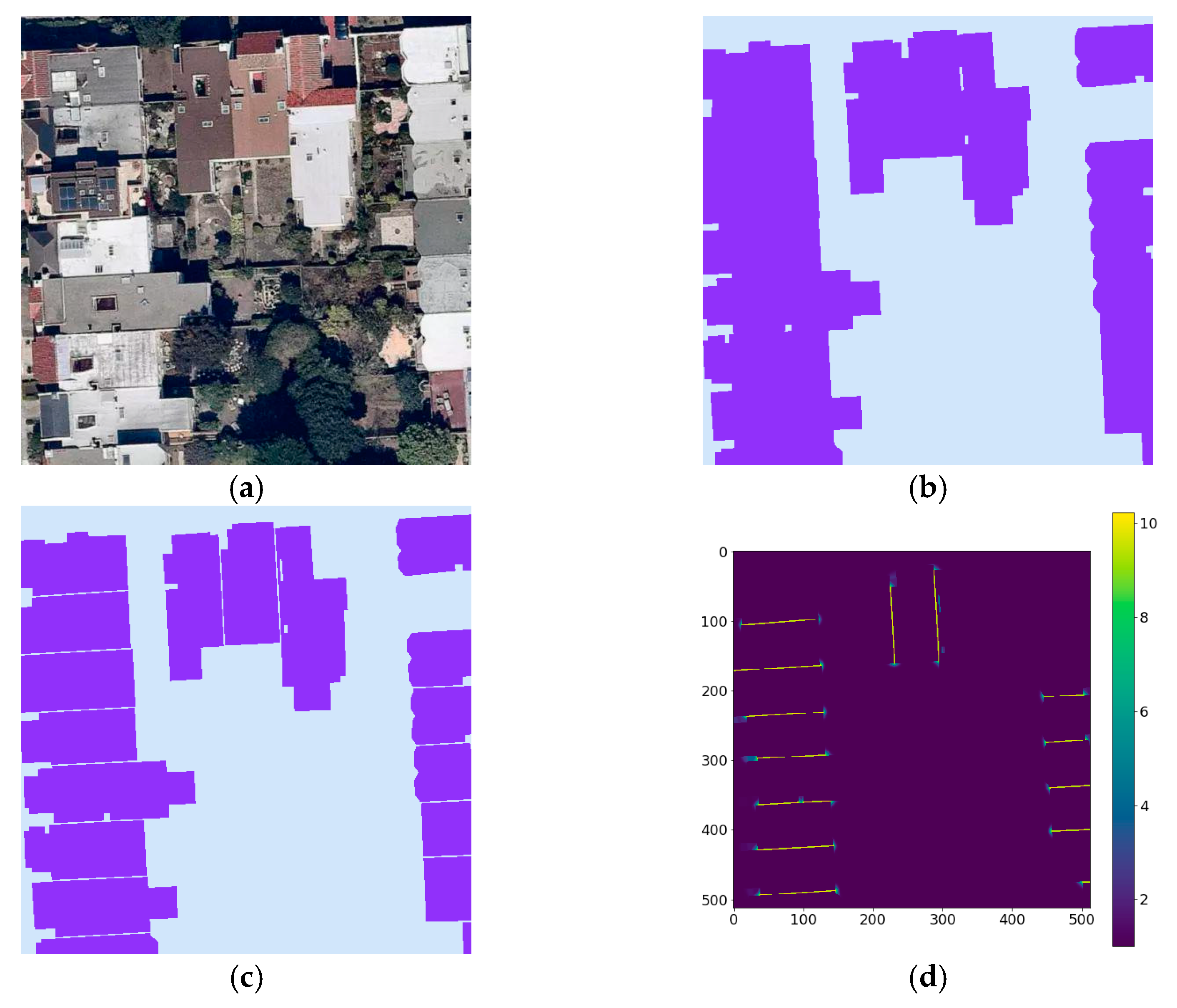
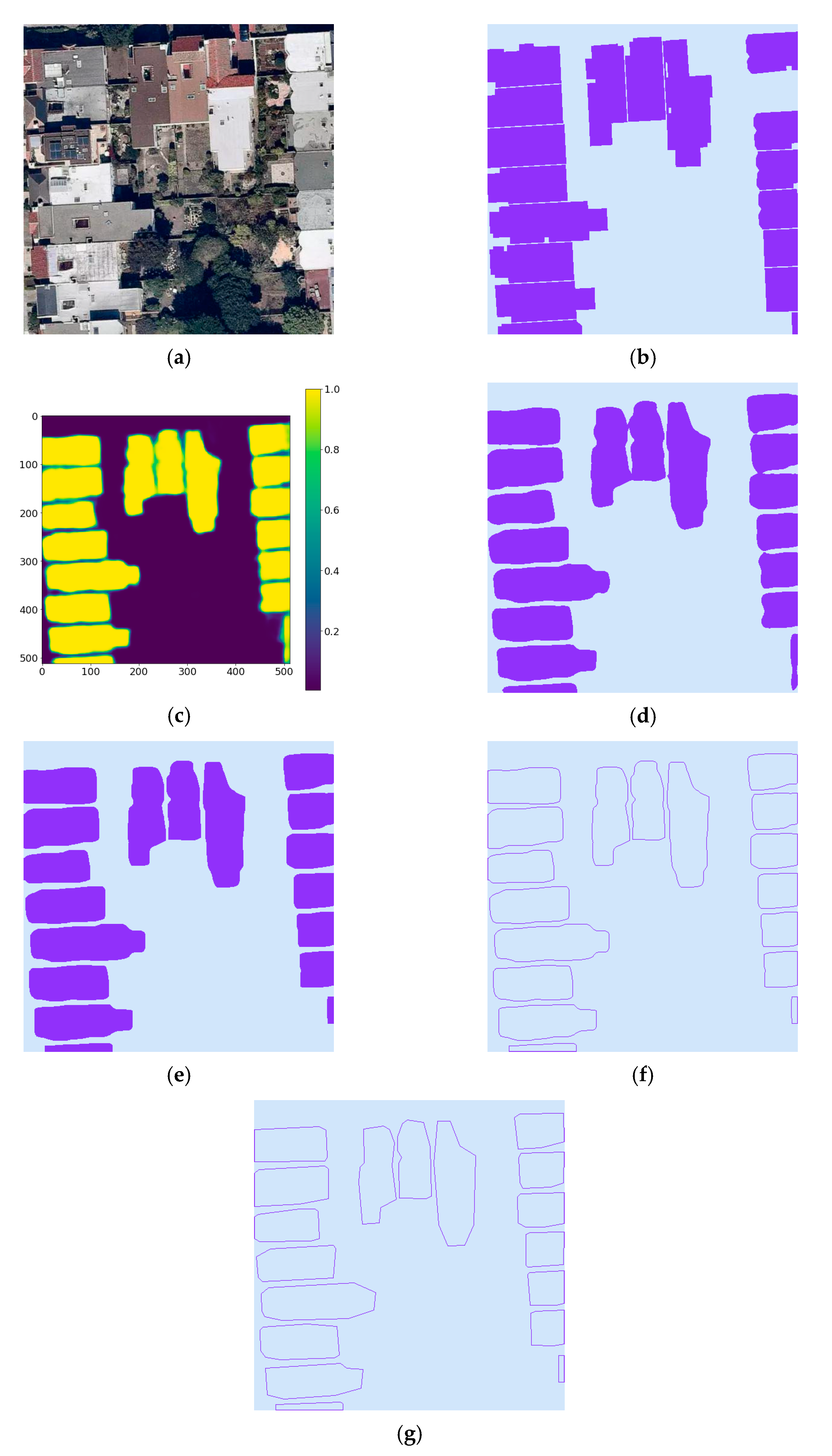
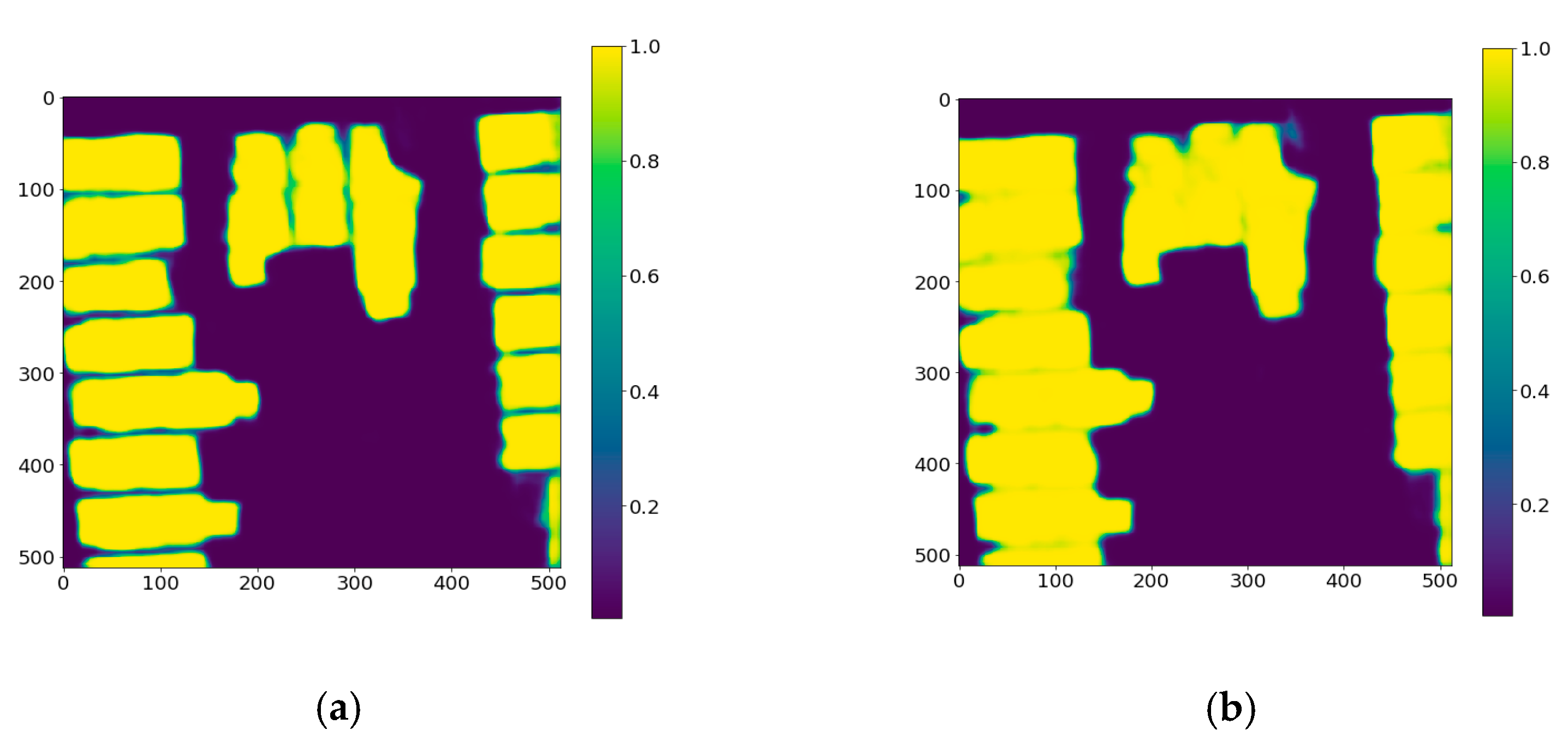
• Converting probability maps into binary masks: The DeepLabv3+ model provides probability masks as outputs, which are converted into a binary mask using 0.5 as a threshold (see an example in Figure 2d).
• Opening morphological operation: this operation is used to remove small objects from the mask while preserving the size and the shape of the larger building footprints (see an example in Figure 2e). This is done by first eroding objects (i.e., remove noise and shrink objects) in the masks and then dilating the eroded objects (i.e., re-expand the objects).
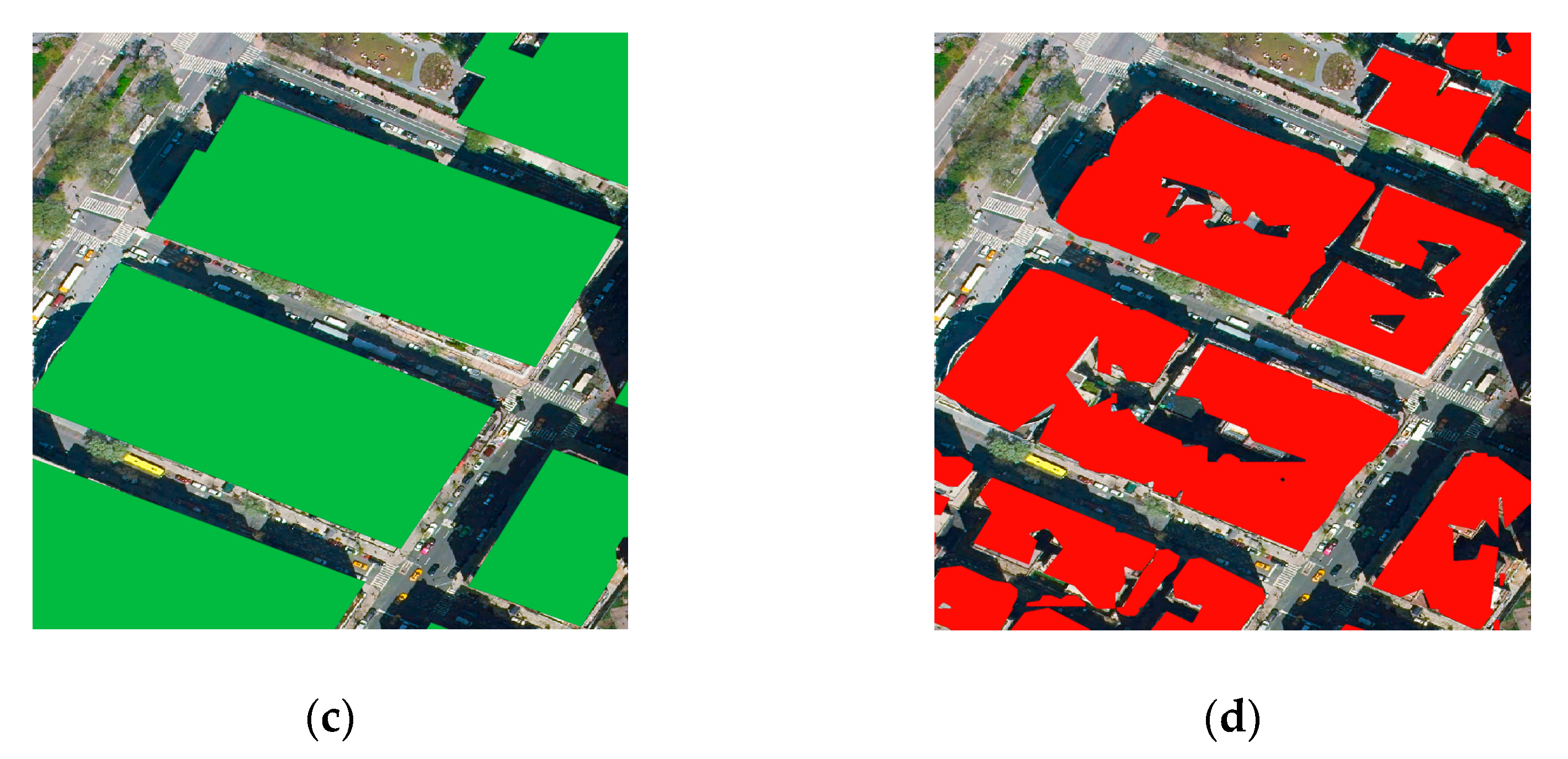
• Polygonization: this is done by detecting the contours of each predicted building footprint, i.e., extracting the curve joining all the pixels having the same color (see an example in Figure 2f).
• Polygon simplification: this step aims to approximate the curve that forms the extracted contour with another curve with fewer vertices (see an example in Figure 2g). The distances between the two curves are less or equal to a precision that is specified by the user. In this work the Douglas-Peucker [35] algorithm was used.
• Converting the polygons’ pixel-based coordinates into geographic coordinates: the result of this step is a GeoJSON GIS file.
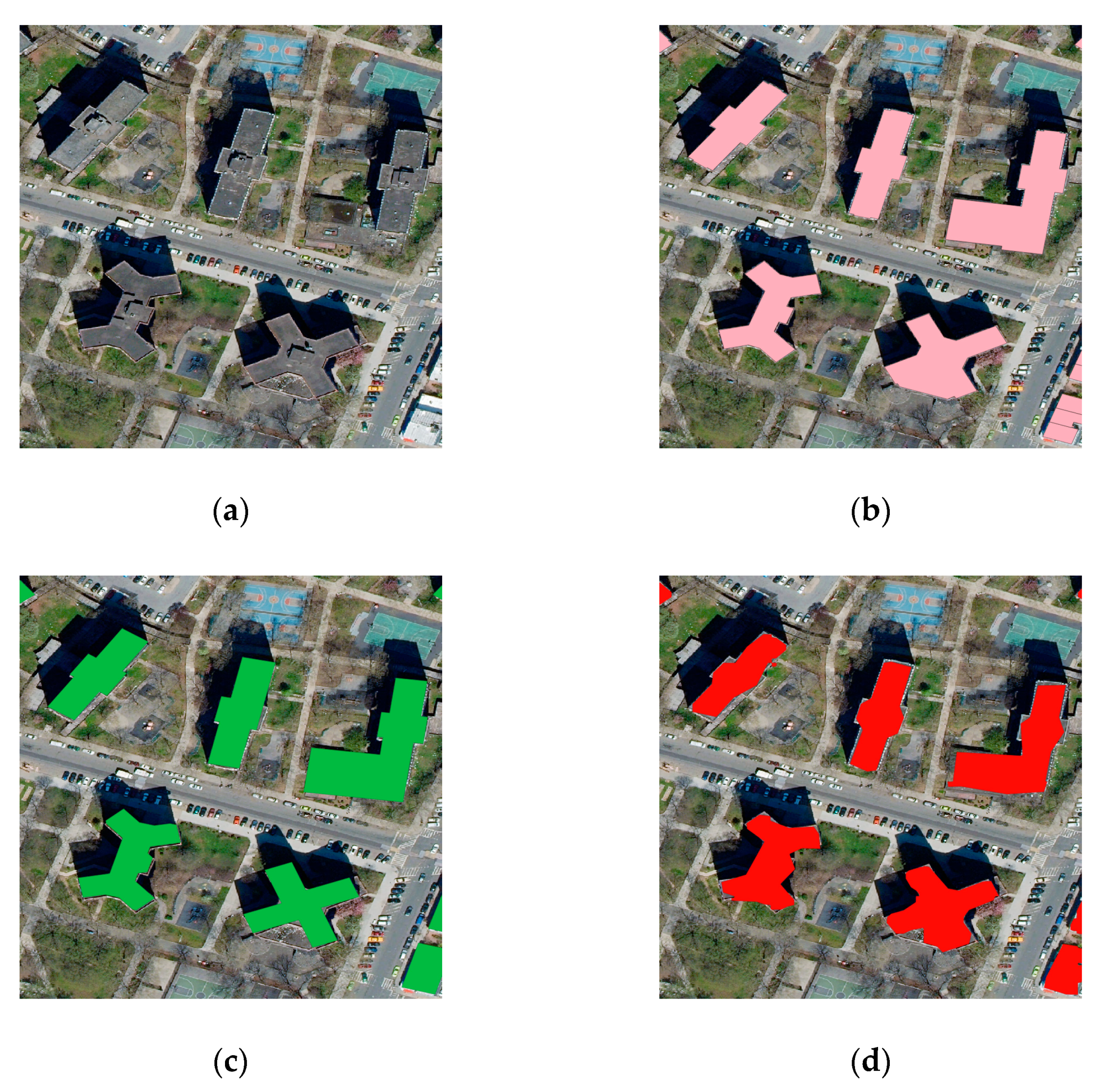
• Polygons merging: in this step polygons that represent the same building footprint, yet were split due to tile boundaries, are merged to obtain a single building footprint.
• Increase the size of each detected polygon (i.e., building footprint): in order to improve the detection of building boundaries that are nearly overlapping, the surface area of each polygon in the training data was decreased by a factor of ~8%. Therefore, the model was trained to underestimate. To overcome this, the reverse operation is applied, and the area of each polygon is increased by 8%.

4. Experiments and Results

The training data was used to train two models. The first model was trained using the loss function defined by Equation (4) in Section 3.2.2 (this model is called dicewce), and the second model used a modified version of this loss function where the spatial weighting was not applied in $L_{CE}$ (this model is called dicece). The accuracy of these two models is compared using the test sample. Using the model that was trained using $L_{dicewce}$ loss function, we generated building footprint predictions using satellite/aerial data from a region of the city of Houston, the entire city of Newark and a region of New York city. Note that while none of Newark and Houston were included in the training process, NY was, which means that 60% of the NY images were used in the training process. The decision to include NY in this analysis is justified by the fact that NY and especially Manhattan is highly dense and has a very specific type of architecture that creates a real challenge to a semantic segmentation approach of detecting building footprint. The resulting footprints were then compared to the building footprints in the dataset released by Microsoft.

4.1. Accuracy Metrics

The semantic segmentation accuracy of the trained models and the Microsoft data is measured using four metrics: mean Intersection over Union (mIoU), F1 score (F1), precision, and recall. These metrics are based on pixel predicted values represented by the total number of true positive (TP), false positive (FP) and false negatives (FN), which are computed using the number of pixels classified as buildings in the predicted masks and in the ground truth masks. Thus:

$$Precision=\frac{TP}{TP+FP}$$

(5)

$$Recall=\frac{TP}{TP+FN}$$

(6)

$$F1=\frac{2TP}{2TP+FP+FN}=2\frac{precision\times recall}{precision+recall}$$

(7)

To compute the mIoU, IoU is first calculated for each class (building and background) then averaged. IoU is defined as:

$$IoU=\frac{TP}{TP+FP+FN}$$

(8)

4.2. Impact of the Spatial Weighting in the Loss Function

Figure 3 shows the convergence during the training process of mIoU, which is the metric used to select the best model; note that the depicted mIoU are computed using the validation sample. One can see that when using dicece as loss function, the models converge faster than using dicewce and has a slightly better mIoU for the best model (the difference between the best dicece and best dicewce models is less than 0.004), which can be explained by the fact that it is harder to learn the boundaries between the adjacent building.

Table 1. Summary of accuracy results using the test sample.

	Precision	Recall	F1 Score	mIoU
dicewce	0.91	0.89	0.90	0.89
dicece	0.90	0.90	0.90	0.89

. shows the building footprint segmentation accuracy metrics of the two trained DeepLabv3+ models (i.e., dicewce and dicece) computed using the test sample. These metrics show no significant difference in term of pixel wise semantic segmentation accuracy between the two models. The main difference is that dicewce has a slightly better performance than dicece in term of precision, while dicece has a slightly better performance in term of recall. However, when a visual analysis is performed of the predicted probabilities maps, it is clear that using the spatial weighting in the loss function significantly improves the detection of the separation between adjacent buildings. Figure 4 shows an example of these probability maps for a densely built region in San Francisco, CA. One can see that the gap between the adjacent buildings has a significantly lower probability of being classified as a building when the dicewce model was used. Figure 4 also show that dicewce is more conservative in labeling pixels between the adjacent buildings, which explains why it has a lower performance in term of recall and a better performance in term of precision in comparison to dicece.

4.3. Comparison with Microsoft Building Footprint Data

The second analysis was performed by using the trained dicewce model to make predictions using the imagery from Newark, NJ and from the previously defined regions of NY city and Houston. The obtained probability maps for these three cities were postprocessed following the pipeline described in Section 3.3. The resulting building footprint GIS files (from step 7 in the postprocessing pipeline) were converted into masks and used to estimate accuracy metrics. Similarly, the Microsoft building footprint GIS files for the same three regions have been used to generate masks, which are used to estimate the accuracy metrics.

The accuracy results of the footprints obtained with the dicewce model and the Microsoft approach are presented in

Table 2. Summary of accuracy results for the three test regions.

	Precision	Newark, NJ	Houston, TX	NY City, NY
DeepLabV3+	Precision	0.88	0.94	0.93
	Recall	0.81	0.75	0.9
	F1 score	0.84	0.83	0.92
	mIoU	0.81	0.81	0.88
Microsoft	Precision	0.88	0.9	0.84
	Recall	0.82	0.76	0.92
	F1 score	0.85	0.82	0.88
	mIoU	0.82	0.79	0.82

The bold is to show the best results (i.e., most accurate).

for the three regions. The proposed approach achieved better results than Microsoft in terms of accuracy metrics for NY city and Houston, while Microsoft footprints are slightly better for Newark.

Table 3. Number of detected footprints.

	Newark, NJ	Houston, TX	NY City, NY
Ground truth	44,853	198,671	120,886
Microsoft	24,930	144,072	20,939
DeepLabV3+	41,409	185,814	47,788

provides a comparison in terms of the number of detected buildings between the proposed approach and Microsoft footprints. One can see that the tested approach significantly outperforms Microsoft results. The number of separate buildings detected by our approach is ~66% higher for Newark, ~29% higher for Houston and ~128% higher for NY city. It is important to note that we have performed an extensive visual inspection of the polygons generated by our method and we have not seen any serious over-segmentation issue.

Figure 5, Figure 6 and Figure 7 provide three examples of comparison between the predicted building footprint produced by the proposed approach and the building footprint provided by Microsoft. In each of these figures, image (a) represents the remote sensing image, image (b) the remote sensing image overlayed with the ground truth mask generated using the gathered GIS files, image (c) the remote sensing image overlayed with the mask generated using the GIS files provided by Microsoft, and finally image (d) the remote sensing image overlayed by the mask generated from the GIS files produced by the proposed approach (using the deep learning model with dicewce loss function). These findings are driven by the fact that the Microsoft approach is not performing well at detecting the separation between buildings and building’s courtyards, as is shown in Figure 5. Most of the time in a densely built environment, the Microsoft approach detects blocks of buildings rather than separate buildings. Our proposed approach performed much better at this task thanks to the employed loss function. However, our model also failed to detect the adjacent buildings’ separation as can be seen in Figure 5 and more dramatically in Figure 6 where the building footprints have more complex shapes. Figure 7 shows a less dense area where Microsoft building footprints have a more realistic shape, which is due to the post processing pipeline that Microsoft used that performs well in producing realistic shapes in areas with lower building density. Figure 6 and Figure 7 show that both approaches fail to accurately predict the boundaries of building footprints.

5. Conclusions

In this work, we described and evaluated an end-to-end approach for building footprint extraction from remote sensing images, which is based on deep semantic segmentation. The proposed workflow consists of three steps: data preprocessing, modeling, and results postprocessing. The data preprocessing step takes advantage of openly available building footprint GIS data to automatically generate ground truth masks that can be used for training. This addresses one of the most challenging aspects of deep learning based semantic segmentation–generating a sufficient amount of labeled training data. The second step of the workflow is the deep semantic segmentation modeling (i.e., model training). In this work we applied the state-of-the-art DeepLabv3+ semantic segmentation algorithm. The last step of the workflow is the semantic segmentation results postprocessing, which transforms the extracted building footprints into GIS format.

The developed approach was evaluated using data gathered from 15 cities and five counties, with promising results when compared to an existing yet closed, best-in-class solution from Microsoft. These encouraging results were obtained in spite of using noisy data with imperfect ground truth masks (i.e., ground truth masks in comparison to remote sensing images). These discrepancies were due to a difference in the vintage of the imagery and the building footprint records. Additional performance improvements might be gained if these discrepancies can be removed from the training dataset. One of the major weaknesses of the proposed approach is that it fails to predict accurate building boundaries. The predicted building footprints do not have regular shapes, as do actual building footprints. This is likely to be due to the fact that the semantic segmentation modeling approach and the post processing steps are not constrained by the building geometry. The noisy data that is used may also have an impact on the shapes’ prediction accuracy.

Although the proposed approach was applied to building footprint extraction, it is possible to adapt the workflow to several other semantic segmentation tasks that are relevant to building energy applications, such as detecting the presence of photovoltaic panels, and packaged rooftop heating ventilation and air conditioning systems, especially as a high accuracy in detection of the shape of these objects is usually not as important as getting a descent accuracy of their size, which will be used as a proxy for extracting some energy related characteristics (e.g., energy production for photovoltaic panels). However, it is important to note that to the best of our knowledge there are no extensive open sources of GIS data that localize these types of objects. In addition, urban planning applications could benefit from the use of these techniques for road and vegetation detection.

Building upon the work presented in this paper, our future work will focus on improving the pipeline to obtain more realistic building footprints. This may involve improving the postprocessing module, or creating a solution to automatically clean the training data (e.g., automatically exclude tiles that have mismatch between ground truth mask and the remote sensing images), developing deep learning models that are more robust to noise. Another direction of our future research will be to explore the usage of Lidar data [36,37,38] in combination with remote sensing RGB images to improve building shape detection and, at the same time, provide estimates of building heights.

References

1. Robinson, C.; Hohman, F.; Dilkina, B. A deep learning approach for population estimation from satellite imagery. In Proceedings of the 1st ACM SIGSPATIAL Workshop on Geospatial Humanities, New York, NY, USA, 7–10 November 2017; pp. 47–54. [Google Scholar]
2. Rodriguez, A.C.; Wegner, J.D. Counting the uncountable: Deep semantic density estimation from space. In German Conference on Pattern Recognition; Springer: Cham, Switzerland, 2018; pp. 351–362. [Google Scholar]
3. Chen, Y.; Hong, T.; Luo, X.; Hooper, B. Development of City Buildings Dataset for Urban Building Energy Modeling. Energy Build. 2019, 183, 252–265. [Google Scholar] [CrossRef] [Green Version]
4. Wang, N.; Goel, S.; Makhmalbaf, A. Commercial Building Energy Asset Score Program Overview and Technical Protocol (Version 1.1); Technical Report, PNNL-22045 Rev. 1.1.; Pacific Northwest National Laboratory: Richland, WA, USA, August 2013.
5. Yu, M.; Yang, C.; Li, Y. Big data in natural disaster management: A review. Geosciences 2018, 8, 165. [Google Scholar] [CrossRef] [Green Version]
6. Cerovecki, A.; Gharahjeh, S.; Harirchian, E.; Ilin, D.; Okhotnikova, K.; Kersten, J. Evaluation of Change Detection Techniques using Very High Resolution Optical Satellite Imagery. Preface 2015, 2, 20. [Google Scholar]
7. Oludare, V.; Kezebou, L.; Panetta, K.; Agaian, S. Semi-supervised learning for improved post-disaster damage assessment from satellite imagery. In Multimodal Image Exploitation and Learning 2021; International Society for Optics and Photonics: Bellingham, WA, USA, 2021; Volume 11734, p. 117340O. [Google Scholar]
8. He, H.; Yang, D.; Wang, S.; Wang, S.; Li, Y. Road extraction by using atrous spatial pyramid pooling integrated encoder-decoder network and structural similarity loss. Remote Sens. 2019, 11, 1015. [Google Scholar] [CrossRef] [Green Version]
9. Lin, Y.; Xu, D.; Wang, N.; Shi, Z.; Chen, Q. Road Extraction from Very-High-Resolution Remote Sensing Images via a Nested SE-Deeplab Model. Remote Sens. 2020, 12, 2985. [Google Scholar] [CrossRef]
10. Sharifzadeh, S.; Tata, J.; Sharifzadeh, H.; Tan, B. Farm Area Segmentation in Satellite Images Using DeepLabv3+ Neural Networks. In International Conference on Data Management Technologies and Applications; Springer: Cham, Switzerland, 2019; pp. 115–135. [Google Scholar]
11. Shrestha, S.; Vanneschi, L. Improved fully convolutional network with conditional random fields for building extraction. Remote Sens. 2018, 10, 1135. [Google Scholar] [CrossRef] [Green Version]
12. Kang, W.; Xiang, Y.; Wang, F.; You, H. EU-Net: An Efficient Fully Convolutional Network for Building Extraction from Optical Remote Sensing Images. Remote Sens. 2019, 11, 2813. [Google Scholar] [CrossRef] [Green Version]
13. Liu, Y.; Gross, L.; Li, Z.; Li, X.; Fan, X.; Qi, W. Automatic building extraction on high-resolution remote sensing imagery using deep convolutional encoder-decoder with spatial pyramid pooling. IEEE Access. 2019, 7, 128774–128786. [Google Scholar] [CrossRef]
14. Ji, S.; Wei, S.; Lu, M. A scale robust convolutional neural network for automatic building extraction from aerial and satellite imagery. Int. J. Remote Sens. 2019, 40, 3308–3322. [Google Scholar] [CrossRef]
15. Valentijn, T.; Margutti, J.; van den Homberg, M.; Laaksonen, J. Multi-Hazard and Spatial Transferability of a CNN for Automated Building Damage Assessment. Remote Sens. 2020, 12, 2839. [Google Scholar] [CrossRef]
16. Bai, Y.; Hu, J.; Su, J.; Liu, X.; Liu, H.; He, X.; Meng, S.; Mas, E.; Koshimura, S. Pyramid Pooling Module-Based Semi-Siamese Network: A Benchmark Model for Assessing Building Damage from xBD Satellite Imagery Datasets. Remote Sens. 2020, 12, 4055. [Google Scholar] [CrossRef]
17. Van Etten, A.; Lindenbaum, D.; Bacastow, T.M. Spacenet: A remote sensing dataset and challenge series. arXiv 2018, arXiv:1807.01232. [Google Scholar]
18. Maggiori, E.; Tarabalka, Y.; Charpiat, G.; Alliez, P. Can semantic labeling methods generalize to any city? Th Inria aerial image labeling benchmark. In Proceedings of the 2017 IEEE International Geoscience and Remote Sensing Symposium (IGARSS), Fort Worth, TX, USA, 23–28 July 2017; pp. 3226–3229. [Google Scholar]
19. Schiefelbein, J.; Rudnick, J.; Scholl, A.; Remmen, P.; Fuchs, M.; Müller, D. Automated urban energy system modeling and thermal building simulation based on OpenStreetMap data sets. Build. Environ. 2019, 149, 630–639. [Google Scholar] [CrossRef]
20. Brovelli, M.; Zamboni, G. A new method for the assessment of spatial accuracy and completeness of OpenStreetMap building footprints. ISPRS Int. J. Geoinf. 2018, 7, 289. [Google Scholar] [CrossRef] [Green Version]
21. Touzani, S.; Wudunn, M.; Zakhor, A.; Pritoni, M.; Singh, R.; Bergmann, H.; Granderson, J. Machine Learning for Automated Extraction of Building Geometry. In Proceedings of the ACEEE Summer Study on Energy Efficiency in Buildings, Pacific Grove, CA, USA, 17–21 August 2020. [Google Scholar]
22. Mapbox 2019. Available online: https://docs.mapbox.com/ (accessed on 25 September 2019).
23. Mapbox, 2018. Available online: https://www.openstreetmap.org/user/pratikyadav/diary/43954. (accessed on 7 December 2020).
24. OSM Wiki: Slippy Map 2020. Available online: https://wiki.openstreetmap.org/wiki/Slippy_Map (accessed on 15 September 2020).
25. USBuildingFootprints, 2018. Microsoft. Available online: https://github.com/microsoft/USBuildingFootprints. (accessed on 10 March 2020).
26. Long, J.; Shelhamer, E.; Darrell, T. Fully convolutional networks for semantic segmentation. In Proceedings of the IEEE Conference on Computer Vision and Pattern Recognition, Boston, MA, USA, 7–12 June 2015; pp. 3431–3440. [Google Scholar]
27. Ronneberger, O.; Fischer, P.; Brox, T. U-net: Convolutional networks for biomedical image segmentation. In International Conference on Medical Image Computing and Computer-Assisted Intervention; Springer: Cham, Switzerland, 2015; pp. 234–241. [Google Scholar]
28. Badrinarayanan, V.; Handa, A.; Cipolla, R. Segnet: A deep convolutional encoder-decoder architecture for robust semantic pixel-wise labelling. arXiv 2015, arXiv:1505.07293. [Google Scholar]
29. Chen, L.C.; Zhu, Y.; Papandreou, G.; Schroff, F.; Adam, H. Encoder-decoder with atrous separable convolution for semantic image segmentation. In Proceedings of the European Conference on Computer Vision (ECCV), Munich, Germany, 8–14 September 2018; pp. 801–818. [Google Scholar]
30. Russakovsky, O.; Deng, J.; Su, H.; Krause, J.; Satheesh, S.; Ma, S.; Huang, Z.; Karpathy, A.; Khosla, A.; Bernstein, M.; et al. Imagenet large scale visual recognition challenge. Int. J. Comput. Vis. 2015, 115, 211–252. [Google Scholar] [CrossRef] [Green Version]
31. He, K.; Zhang, X.; Ren, S.; Sun, J. Deep residual learning for image recognition. In Proceedings of the IEEE Conference on Computer Vision and Pattern Recognition, Las Vegas, NV, USA, 26 June–1 July 2016; pp. 770–778. [Google Scholar]
32. Sudre, C.H.; Li, W.; Vercauteren, T.; Ourselin, S.; Cardoso, M.J. Generalised dice overlap as a deep learning loss function for highly unbalanced segmentations. In Deep Learning in Medical Image Analysis and Multimodal Learning for Clinical Decision Support; Springer: Cham, Switzerland, 2017; pp. 240–248. [Google Scholar]
33. Kingma, D.P.; Ba, J. Adam: A method for stochastic optimization. arXiv 2014, arXiv:1412.6980. [Google Scholar]
34. Ng, V.; Hofmann, D. Scalable Feature Extraction with aerial and Satellite Imagery. In Proceedings of the 17th Python in Science Conference (SCIPY 2018), Austin, TX, USA, 9–15 July 2018; pp. 145–151. [Google Scholar]
35. Douglas, D.H.; Peucker, T.K. Algorithms for the reduction of the number of points required to represent a digitized line or its caricature. Cartogr. Int. J. Geogr. Inf. Geovis. 1973, 10, 112–122. [Google Scholar] [CrossRef] [Green Version]
36. Awrangjeb, M.; Ravanbakhsh, M.; Fraser, C.S. Automatic detection of residential buildings using LIDAR data and multispectral imagery. ISPRS J. Photogramm. Remote. Sens. 2010, 65, 457–467. [Google Scholar] [CrossRef] [Green Version]
37. Awrangjeb, M.; Fraser, C.S. Automatic segmentation of raw LiDAR data for extraction of building roofs. Remote Sens. 2014, 6, 3716–3751. [Google Scholar] [CrossRef] [Green Version]
38. Awrangjeb, M.; Zhang, C.; Fraser, C.S. Building detection in complex scenes thorough effective separation of buildings from trees. Photogramm. Eng. Remote Sens. 2012, 78, 729–745. [Google Scholar] [CrossRef] [Green Version]
Figure 1. Illustration of the data preparation process. (a) Remote sensing image; (b) Ground truth mask; (c) Ground truth mask after downsizing polygons; (d) Spatial weights map.
Remotesensing 13 02578 g001
Figure 2. Example of steps 1 to 4 of the postprocessing. (a) Remote sensing image; (b) scaled ground truth mask; (c) predicted probabilities map; (d) converted binary mask; (e) mask after morphological operation; (f) result of mask polygonization; (g) polygons after simplification.
Remotesensing 13 02578 g002
Figure 3. Convergence of the computed mIoU using validation sample.
Remotesensing 13 02578 g003
Figure 4. Example of probability maps generated by (a) the DeepLabv3+ model using dicewce loss function; (b) the DeepLabv3+ model using dicece loss function.
Remotesensing 13 02578 g004
Figure 5. (a) Remote sensing image; (b) Remote sensing image overlayed with the ground truth mask; (c) Remote sensing image overlayed with the Microsoft predicted building footprints; (d) Remote sensing image overlayed with the predicted footprints using the proposed workflow based on DeepLabv3+ model (using dicewce loss function).
Remotesensing 13 02578 g005
Figure 6. (a) Remote sensing image; (b) Remote sensing image overlayed with the ground truth mask; (c) Remote sensing image overlayed with the Microsoft predicted building footprints; (d) Remote sensing image overlayed with the predicted footprints using the proposed workflow based on DeepLabv3+ model (using dicewce loss function).
Remotesensing 13 02578 g006aRemotesensing 13 02578 g006b
Figure 7. (a) Remote sensing image; (b) Remote sensing image overlayed with the ground truth mask; (c) Remote sensing image overlayed with the Microsoft predicted building footprints; (d) Remote sensing image overlayed with the predicted footprints using the proposed workflow based on DeepLabv3+ model (using dicewce loss function).
Remotesensing 13 02578 g007