Abstract
Recently, deep learning has been successfully and widely used in hyperspectral image (HSI) classification. Considering the difficulty of acquiring HSIs, there are usually a small number of pixels used as the training instances. Therefore, it is hard to fully use the advantages of deep learning networks; for example, the very deep layers with a large number of parameters lead to overfitting. This paper proposed a dynamic wide and deep neural network (DWDNN) for HSI classification, which includes multiple efficient wide sliding window and subsampling (EWSWS) networks and can grow dynamically according to the complexity of the problems. The EWSWS network in the DWDNN was designed both in the wide and deep direction with transform kernels as hidden units. These multiple layers of kernels can extract features from the low to high level, and because they are extended in the wide direction, they can learn features more steadily and smoothly. The sliding windows with the stride and subsampling were designed to reduce the dimension of the features for each layer; therefore, the computational load was reduced. Finally, all the weights were only from the fully connected layer, and the iterative least squares method was used to compute them easily. The proposed DWDNN was tested with several HSI data including the Botswana, Pavia University, and Salinas remote sensing datasets with different numbers of instances (from small to big). The experimental results showed that the proposed method had the highest test accuracies compared to both the typical machine learning methods such as support vector machine (SVM), multilayer perceptron (MLP), radial basis function (RBF), and the recently proposed deep learning methods including the 2D convolutional neural network (CNN) and the 3D CNN designed for HSI classification.
1. Introduction
Hyperspectral images (HSIs) can be viewed as 3D data blocks, which contain abundant 2D spatial information and hundreds of spectral bands. Therefore, they can be used to recognize different materials based on the pixels. These images have been used widely in many applications such as natural resource monitoring, geological mapping, and object detection [1]. Different machine learning methods have been used and proposed for HSI classification in the past few decades, which mainly include supervised learning methods such as probabilistic approaches: multinomial logistic regression (MLR) [2], SVM [3], decision trees [4], MLP [5], random forest (RF) [6], and sparse representation classifiers [7].
Recently, deep learning methods have been introduced for HSI classification to combine both spatial and spectral features [8,9,10,11,12,13,14]. Considering the size of the pixel patches, the deep learning models are usually not very deep. A five-layer CNN [9] was proposed, which combined various properties including batch normalization, dropout, and the parametric rectified linear unit (PReLU) activation function. The local contextual features were also learned by the CNN [8] and diverse region-based CNN [13] to improve the performance. Different features such as multiscale features [11], multiple morphological profiles [10], and diversified metrics [15] were learned by different CNNs. The CNN was also extended to three dimensions such as the 3D CNN [16], mixed CNN [17], and hybrid spectral CNN (HybridSN) [18]. As new methods such as the fully convolutional network (FCN), attention mechanism, active learning, and transfer learning have been proposed and used successfully in computer vision problem, they have also been applied to HSI classification. These learning methods include the FCN with an efficient nonlocal module (ENL-FCN), active learning methods [19,20], 3D octave convolution with the spatial–spectral attention network (3DOC-SSAN) [21], the CNN [22] with transfer learning that uses an unsupervised pre-training step, the superpixel pooling convolutional neural network with transfer learning [23], and the lightweight spectral–spatial attention network [24]. Researchers have also tried to learn features more efficiently and robustly using the proxy-based deep learning framework [25].
Other than CNNs, new technologies have also been applied to HSI classification, such as the deep recurrent neural network [26] and spectral–spatial attention networks based on the RNN and CNN learning spectral correlations within a continuous spectrum and spatial neighboring relevance. The deep support vector machine (DSVM) [27] extended the SVM in the deep direction. Harmonic networks [28] were proposed using circular harmonics instead of CNN kernels. These were extended as naive Gabor networks [29] for HSI classification, which can reduce the number of learning parameters. A cascaded dual-scale crossover network [30] was proposed to extract more features without extending the architecture in the deep direction. Recently, a recurrent feedback convolutional neural network [31] was proposed to overcome overfitting, and a generative adversarial minority oversampling method [32] was proposed to deal with imbalanced data in HSIs.
It is usually not efficient to train a learning model with a large number of training samples with a single HSI dataset. Therefore, this is the drawback of using deep learning models with a large amount of hyperparameters and layers. Incremental learning is learning new knowledge without forgetting learned knowledge to overcome catastrophic forgetting [33]. It can also make the learning model be generated according to the complexity of the learning models, which is useful for HSI classification with limited training samples. Researcher have proposed different incremental methods such as elastic weight consolidation (EWC) [34], remembering old knowledge by selectively reducing important weights, and incremental moment matching (IMM) [35], assuming that the posterior distribution of the parameters of the Bayesian neural networks matches the moment of the posteriors incrementally. Another similar idea is scalable learning, which mainly includes multistage scalable learning and tree-like scalable learning. The parallel, self-organizing, hierarchical neural networks (PSHNNs) [36] and parallel consensual neural networks (PCNNs) [37] have been proposed, which usually combine multiple stages of neural networks with an instance rejection mechanism or statistical consensus theory. The final output of these networks is the consensus result among all the stages of the neural networks. Scalable-effort classifiers [38,39] were proposed including multiple stages of classifiers, which can be increased with increasing architectural complexity. A Tree-CNN was proposed [40], and the deep learning models were organized hierarchically to learn incrementally. Conditional deep learning (CDL) [41] was proposed for the active convolutional layer for inputs that hard to classify. Stochastic configuration networks (SCNs) [42] were proposed using a stochastic configuration to grow the hidden units incrementally. Other than different types of learning methods, researchers proposed methods on learning security such as adversarial examples [43] and the backdoor attack on multiple learning models [44].
In addition to the deep direction, the learning model can be generated in wide [45,46] or both wide and deep [47] directions. It was discovered that the training and learning process of the wide fully connected neural networks can be represented by the evaluation of the Gaussian process, and the wide neural network usually has better performance in generalization [45,46]. Recently, researchers also tried to combine HSI with LiDAR data to perform land cover classification, such as discriminant correlation analysis [48] and the inverse coefficient of variation features and multilevel fusion method [49].
In this paper, we proposed a dynamic wide and deep neural network (DWDNN) for hyperspectral image classification, which combines wide and deep learning and generates the learning model with the proper architectural complexity for different learning data and tasks. It was based on multiple dynamically organized efficient wide sliding windows and subsampling (EWSWS) networks. Each EWSWS network has multiple layers of transform kernels with sliding windows and strides, which can be extended in the wide direction to learn both the spatial and spectral features sufficiently. The parameters of these transform kernels can be learned with randomly chosen training samples, and the number of the outputs of the transform kernels can be reduced. With multiple EWSWS layers combined in the deep direction, the spatial and spectral features from the lower level to the higher level can be learned efficiently with a proper configuration of the hyperparameters for EWSWS networks. The EWSWS network can be generated one-by-one dynamically. In this way, the DWDNN can learn features from HSI data more smoothly and efficiently to overcome overfitting. The weights of the DWDNN are mainly in the fully connected layer, which can be learned easily using iterative least squares. The contributions of the proposed DWDNN are as follows:
- Extracting spatial and spectral features from the low level to the high level efficiently by the EWSWS network with a proper architectural complexity;
- Training the DWDNN easily, because the parameters of the transform kernels in EWSWS networks can be obtained directly by randomly choosing training samples or with the unsupervised learning method. The only weights are those in the fully connected layers, which can be computed with iterative least squares;
- Generating learning models with the proper architectural complexity according to the characteristics of the HSI data. Therefore, learning can be more efficient and smooth.
The rest of the paper is organized as follows: Section 2 presents the detailed description of the proposed DWDNN. Section 3 presents the datasets and the experimental settings. Section 4 gives the classification results for the HSI data. Section 5 and Section 6 provide the discussions and conclusions.
2. Dynamic Wide and Deep Neural Network for Hyperspectral Image Classification
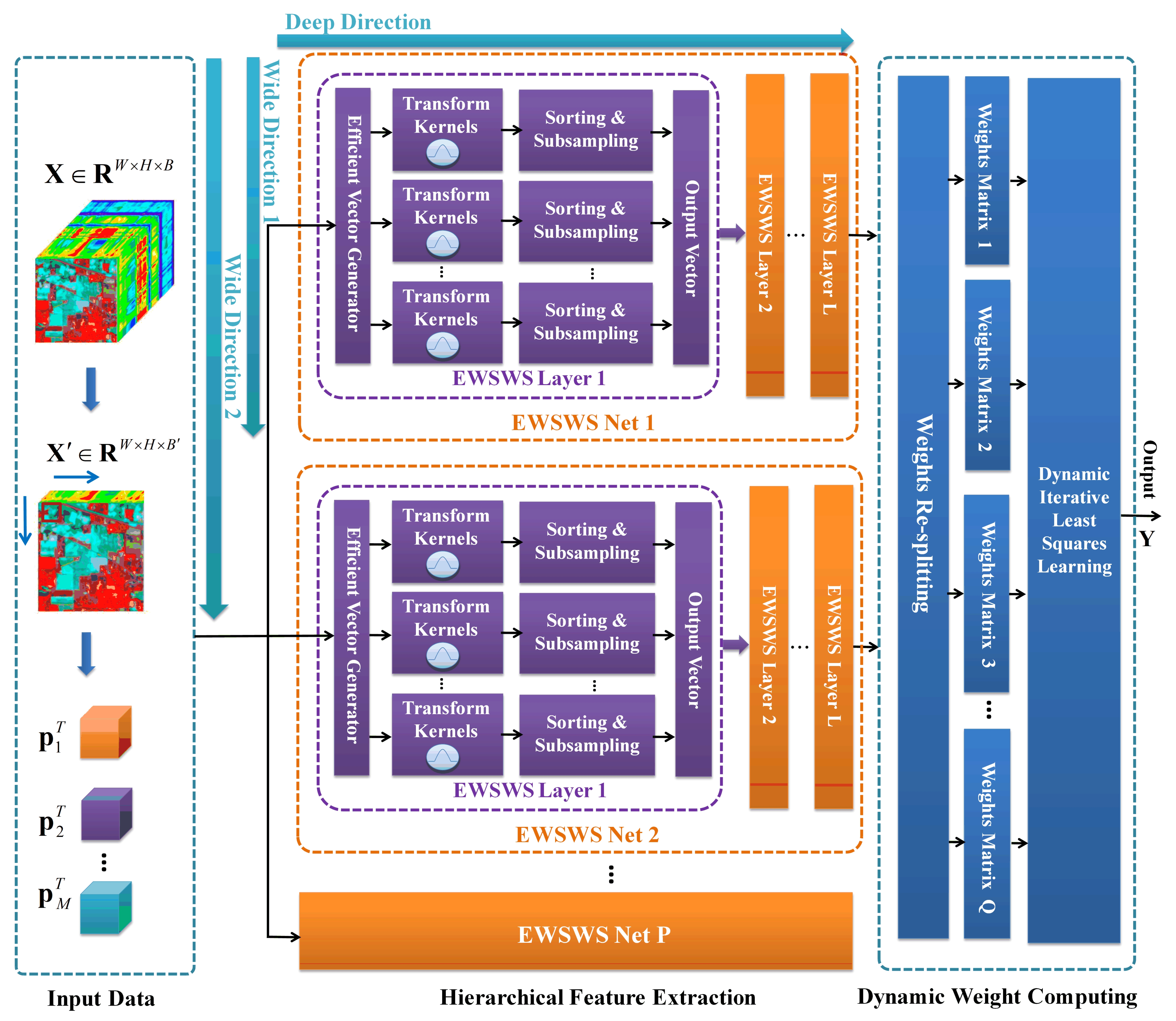
The DWDNN mainly includes the following: (1) hyperspectral image preprocessing; (2) an efficient wide sliding window and subsampling (EWSWS) network; and (3) the dynamic growth of the wide and deep neural network. The architecture of the DWDNN is shown in Figure 1.
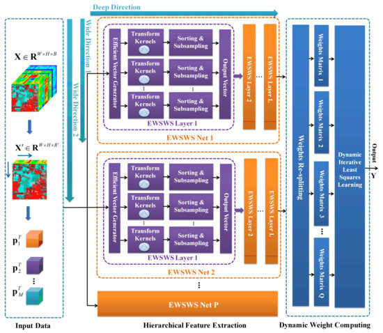
Figure 1.
Architecture of the DWDNN. The DWDNN is composed of multiple EWSWS networks, which are generated in the wide direction. Each EWSWS network has L layers of transform kernels with sliding windows and strides in the deep direction. Each WSWS layer can be extended in the wide direction. Therefore, the DWDNN can learn features effectively with both the wide and deep architecture. The parameters of these transform kernels can be learned with randomly chosen training samples. The weights of the DWDNN are mainly in the fully connected layer and can be learned easily using iterative least squares.
2.1. Hyperspectral Image Preprocessing and Instances’ Preparation
Suppose the HSI data are , where W, H, and B are the width, height, and number of bands in the HSI data. Principal component analysis (PCA) was performed to reduce the redundant spectral information firstly, and data normalization was implemented. Suppose the number of classes is C. The image patches after PCA can be generated with a size of . These image patches were split into training, validation, and testing instances with the corresponding splitting ratios. The image patches were flattened into vectors. The sliding window was used to generate the input subvectors with a given stride to reduce the computational load. The strides can be adjusted with different scopes. These strides can reduce the number of generated RBF networks for the EWSWS network to save on the computational load if large values can be used. These strides can also be adjusted flexibly to extract features from different levels. The HSI preprocessing process is shown in Figure 2.
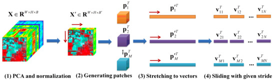
Figure 2.
Hyperspectral image preprocessing and instances’ preparation.
2.2. Efficient Wide Sliding Window and Subsampling Network
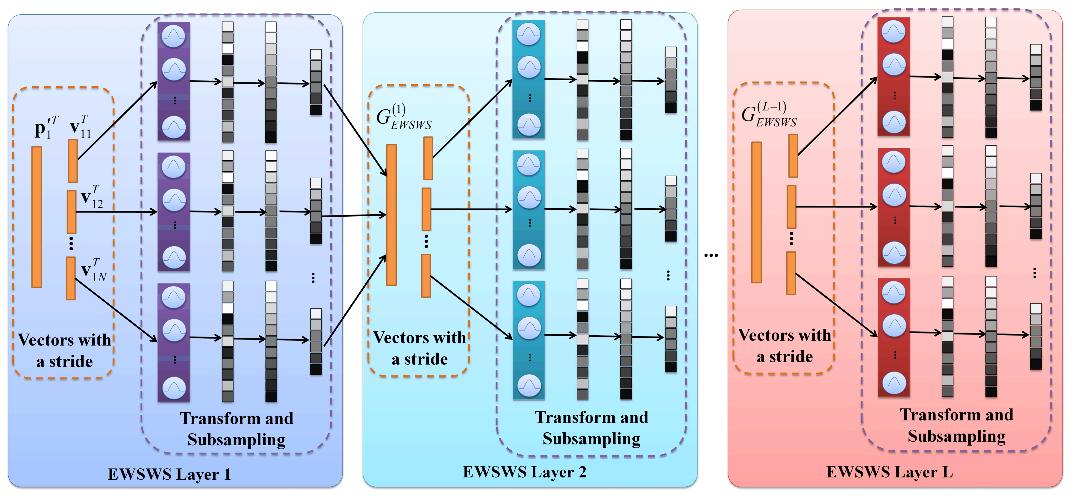
For HSI classification, one key point is how to use a large number of bands efficiently, even though the PCA is usually used to reduce the redundant information. The CNN-based deep learning methods usually combine spatial and spectral features to obtain higher HSI classification performance. However, the limited training samples make it hard to use very deep architectures, and there are a large number of convolutional kernels to be learned. Recently, researcher have used different kernels to enhance the HSI classification performance and reduce the number of learned kernels, such as circular harmonics [28], naive Gabor filters [29], and the recently proposed WSWS network with Gaussian kernels [50]. As we discussed in Section 2.1, in this paper, the strides were combined with the WSWS layers to make them efficient when learning the features of different levels, and the EWSWS layers were generated to learn these bands of images more efficiently. The architecture of the EWSWS layer is shown in Figure 3.
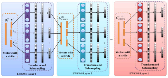
Figure 3.
The architecture of the EWSWS layers. The EWSWS layers are in both the wide and deep direction. Each layer includes the transform kernels, sorting, and subsampling. The sliding window with a stride is used for each layer, and the layer is extended in the wide direction by using these sliding windows.
For HSI classification, the 3D hyperspectral image patches after using PCA are the input to the EWSWS network. Suppose the size of the one-dimensional sliding window is set as w, which denotes the length of the sliding window. The stride s is used to reduce the redundant number of sliding times according to the characteristic of the input data. For the sliding time, the 1D vectors are . They are fed into the EWSWS composed of layers of transform kernels denoted as , where denotes the number of transform kernels for the sliding time. The outputs of the transform kernels from the sliding window are denoted as , representing . In general, suppose there is more than one channel. Then, the summation along the channel direction is performed for each set of transform kernels, which are:
Then, sorting is performed along the sample dimension, and in order to reduce the number of the outputs of the transform kernels, subsampling is performed with the sorted output. These two operations are denoted by:
where is the subsampling interval.
For each sliding window, a set of transformed outputs is generated in the wide direction, and finally, they can be combined together as:
In order to obtain higher level features, the transform layers are extended in the deep direction with multiple transform kernel layers and different strides. Suppose the sets of the outputs of the first layer are . Then, the outputs of the following layers are denoted as:
where is the number of sliding windows in the layer of the transform kernels. For each layer, the strides are denoted as .
Suppose there are L layers. The output of the layer of transform kernels is . The final outputs of the EWSWS network are given by:
The least squares estimation of is computed by minimizing the squared error:
where is the vector of the desired ground truths of the classes.
Finally, the pseudoinverse of is used to compute [51]:
2.3. Dynamic Wide and Deep Neural Network
When the EWSWS layers are extended in both the wide and deep directions, the learning model has the ability to learn high-level features from both the spatial and spectral domain with the HSI data. Unlike the CNN, which uses gradient descent to learn the weights gradually, the least squares method learns all the linear weights once, which is much faster. On the negative side, the learning model may switch between the states of underfitting and overfitting easily if there are no proper hyperparameters for the proposed model. Another problem is that when there are a large number of training samples and the sizes of patches are large, the computing weights need a large number of computing resources.
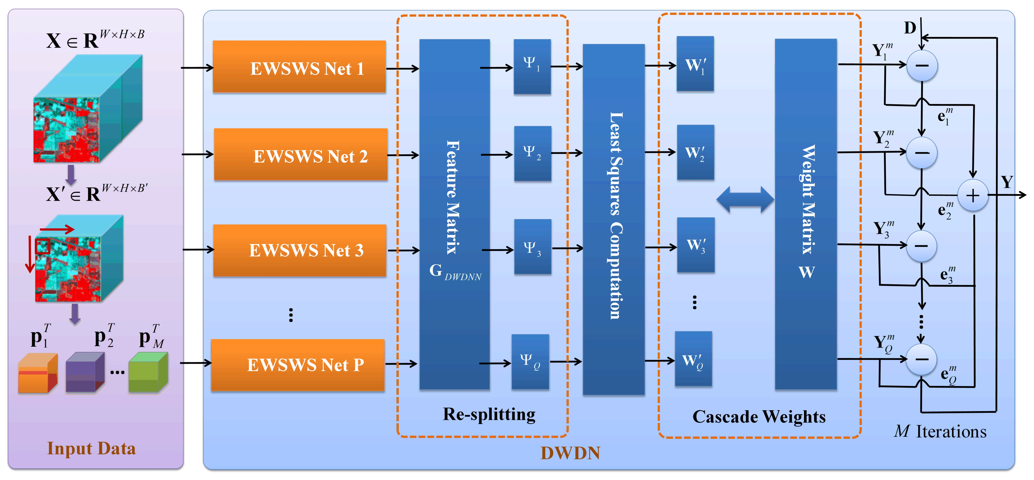
Considering the above issues, the iterative least squares [52] method was combined with EWSWS Nets, and the DWDNN was proposed. Multiple EWSWS networks can be added into the DWDNN one-by-one using iterative least squares to gain more learning ability dynamically. When the training data are learned sufficiently, the growing process is stopped automatically. During this process, the training data are split into both the feature and sample domain; therefore, it can be used for the HSI data with a high feature dimension and a large number of training samples. Another advantage of the DWDNN is that, while finding the proper architecture dynamically, the learning process is much more stable with well-trained weights in the fully connected layer. The dynamic learning process is shown in Figure 4.

Figure 4.
Dynamic iterative learning of the DWDNN. The weights are related to the combined outputs of the final EWSWS layers from the EWSWS networks. The weights’ resplitting block and iterative least squares are used to learn these weights in the fully connected layer.
2.3.1. Data Splitting in the Sample Space
In order to learn the information in the training set sufficiently, training samples are split into a number of batches as in the BP neural network or the CNN, with a proportion of overlap for each training batch, which can be determined by an overlapping factor . For HSI classification, the 3D training patches are split into training subsets with the overlapping factor , which can be described as:
The whole training set can be learned in epochs with the DWDNN using the iterative least squares method. After each training epoch, the training set is shuffled, and the new training batches are split by using the overlapping factor.
2.3.2. Generating the DWDNN Dynamically
In this section, we describe how to generate the DWDNN dynamically. The generating process starts with the first EWSWS network. Then, the succeeding EWSWS Nets are added one by one according to the trained errors of the previous EWSWS Nets. If the problem scale can be estimated, a certain number of EWSWS Nets can be given in advance. Then, the DWDNN can grow quickly to reach the proper number of EWSWS Nets. Suppose the first EWSWS network is and the first subset is used to train it. The outputs of the EWSWS layer for the first iteration are . The learning of the desired outputs, the computed weights, and the outputs are as follows:
The remaining error of is:
The second EWSWS network is added to reduce the learning error, and is the output of the EWSWS layers. The learning of the remaining error, the computed weights, and the outputs are given by:
The remaining error of is:
A desired error threshold and the maximum number of EWSWS networks for the DWDNN denoted as are given as required according to the learning tasks. The succeeding EWSWS networks can be generated one-by-one until the remaining error is less than or the number of EWSWS networks reaches the maximum number . Suppose EWSWS networks were generated in the first iteration. Then, the second training subset is used to train the current DWDNN. Using , the learning of the remaining error during the first iteration, the computed weights, and the outputs are given by:
The remaining error of for the second iteration is:
The weights are updated for the succeeding EWSWS Nets, and the remaining error of for the second iteration is:
Then, EWSWS networks are added until the remaining error is less than or the number of EWSWS Nets reaches the maximum number . The succeeding training subsets are used similarly, and EWSWS Nets are generated and combined as the final DWDNN. If the training set is not very big, a single dataset is enough to train a DWDNN iteratively. During the iterations, the validation set can also be used to stop the training to avoid overfitting.
2.3.3. Weights’ Resplitting Method
Suppose the outputs of the transform kernels of the DWDNN are denoted as , which are also the outputs of EWSWS networks. This can be expressed as:
When the feature dimension of the matrix extracted by EWSWS networks is larger than the number of training samples, the feature matrix is split along the feature dimension to learn more stably. The process can be rewritten as:
Then, is used to compute the weights in the DWDNN.
3. Datasets and Experimental Settings
The HSI datasets Botswana, Pavia University, and Salinas [53] used in the experiments and shown in Table 1 are as follows:

Table 1.
Description of the hyperspectral remote sensing datasets.
(1) Botswana:This was acquired by the NASA EO-1 satellite over the Okavango Delta, Botswana, in 2001–2004. The data have a 30 m pixel resolution over a 7.7 km strip in 242 bands. The spectrum is from 400–2500 nm. After removing the uncalibrated and noisy bands that cover water absorption, one-hundred forty-five bands are included as the candidate features. There are 14 classes of land cover;
(2) Pavia University: The data were acquired by the ROSIS sensor over Pavia. The images are (after discarding the pixels without information, the image is ). There are 9 classes in total in the images;
(3) Salinas: This was obtained in Salinas Valley, California, with 204 bands (abandoning bands of water absorption), and the size is . There are 16 classes in total in the images.
The experiments were performed with a desktop with Intel i7-8700K CPU, NVDIA RTX 2080TI GPU, and 32GB memory. The number of hyperspectral bands was reduced to 15 using principal component analysis. The different patch sizes of the HSIs have different effects on the classification results. The performance usually increases as the size of the patches increases. However the computational load can also increase [21]. Therefore, there is a balance between the patch size and the computational load. We chose as the patch size for all datasets to ensure that the DWDNN could achieve good performance and the computation process was efficient. For the hyperspectral data, there was one channel after the selected bands were concatenated as a vector. The proportions of the instances for training and validation were 0.2 for Pavia University and Salinas. For Botswana, the ratios were 0.14 and 0.01. The training instances were organized together as a single set to train the DWDNN. The patch size for the proposed method was . The remaining instances were used for testing. The overall accuracy (OA), average accuracy (AA), and Kappa coefficient [50] were used to evaluate the performance. The DWDNN was composed of 10 EWSWS networks, and the detailed parameters for each EWSWS network on different datasets are show in Table 2. There are two formats of the parameters for the size of the sliding window: the integers represent the absolute window sizes, and the decimals represent the ratio of the length of the input vectors as the window sizes.
Table 2.
Parameter settings for the DWDNN on different hyperspectral datasets.
4. Performance of Classification with Different Hyperspectral Datasets
For the Botswana dataset, the proposed DWDNN was compared with SVM [21,26], multilayer perceptron (MLP) [50], RBF [50], the CNN [50], the recently proposed 2D CNN [21,26], the 3D CNN [21,26], deep recurrent neural networks (DRNNs) [21,26], and the wide sliding window and subsampling (WSWS) network [50]. MLP was implemented with 1000 hidden units. The RBF network had 100 Gaussian kernels, and the centers of these kernels were chosen randomly from the training instances. The CNN was composed of a convolutional layer with 6 convolutional kernels, a pooling layer (scale 2), a convolutional layer with 12 convolutional kernels, and a pooling layer (scale 2). The patch size was for MLP and RBF and for the CNN.
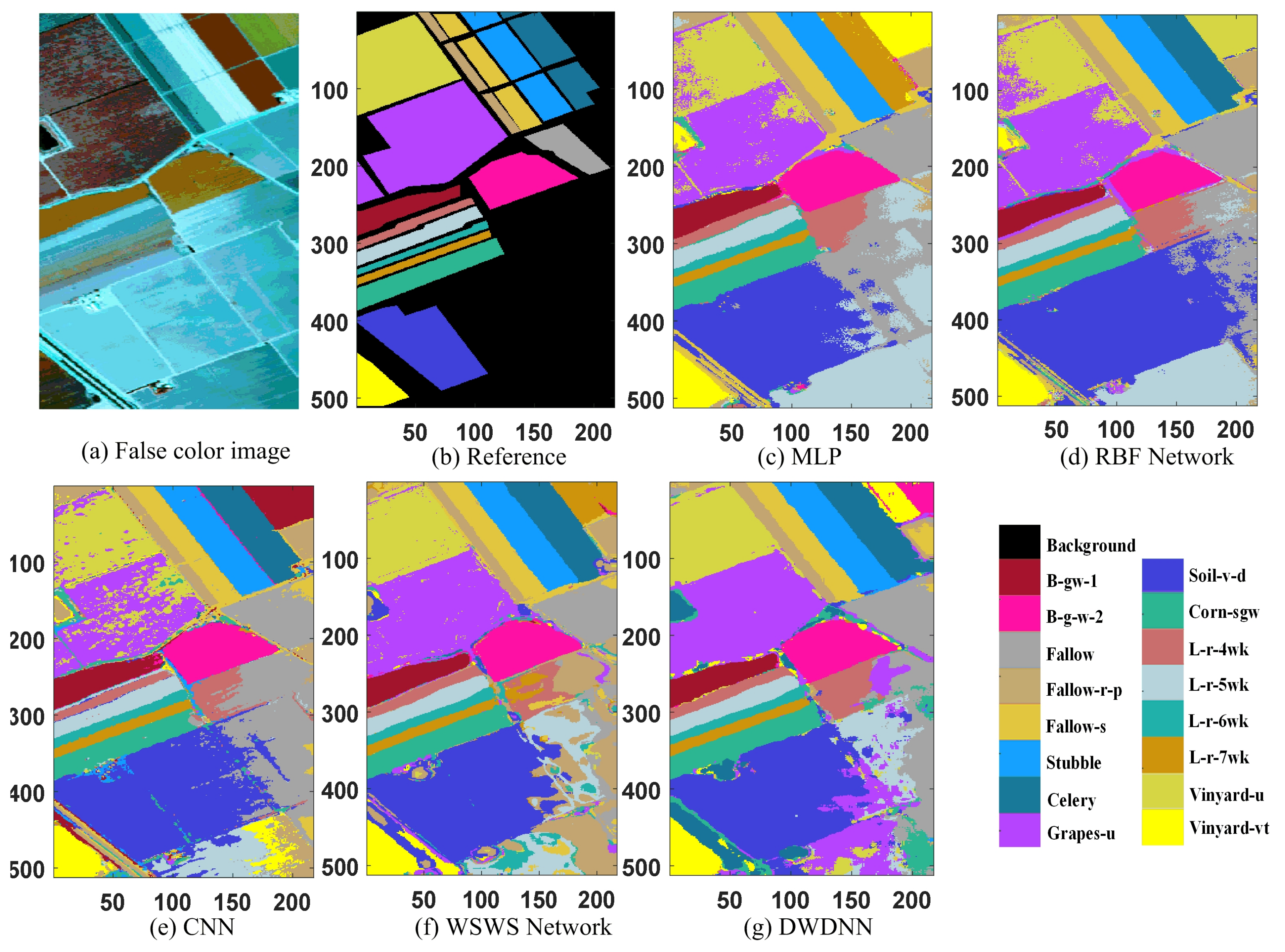
The classification results are shown in Table 3 and Figure 5. The proposed DWDNN had the best OA and Kappa coefficient among the compared methods. The OA, AA, and Kappa coefficient of the DWDNN could reach 99.64%, 99.60%, and 99.61%, respectively. The test accuracy for each class in the table represents how many samples could be classified correctly among the total number of samples in the corresponding class. The test accuracies of 12 of the 14 classes reached 100%. Figure 5 shows the predicted results of the whole hyperspectral image. The proposed DWDNN had much smoother classification results for almost all classes. For example, the class of exposed soils with yellow color in Figure 5g has much smoother connected regions.
Table 3.
Classification results of different methods on the Botswana dataset.
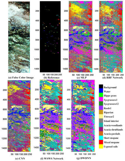
Figure 5.
Classification results of the Botswana dataset (the instances without class information were also predicted). (a) False color image, (b) reference image, (c) MLP, (d) RBF network, (e) CNN, (f) WSWS network, and (g) DWDNN.
For the Pavia University and Salinas datasets, the proposed DWDNN was compared with SVM [17,54], MLP [50], RBF [50], the CNN [50], the 2D CNN [17,55], the 3D CNN [16,17], sparse modeling of spectral blocks (SMSB) [56], and the WSWS Net [50]. MLP had 1000 hidden units. The RBF network had 2000 Gaussian kernels, and the centers of these kernels were chosen randomly from the training instances. The CNN was composed of a convolutional layer with 6 convolutional kernels, a pooling layer (scale 2), a convolutional layer with 12 convolutional kernels, and a pooling layer (scale 2). The patch sizes were for MLP, for RBF, and for the CNN, respectively.
The classification results for the Pavia University dataset are shown in Table 4 and Figure 6. The proposed DWDNN had the highest classification results compared with the other methods. The OA, AA, and Kappa coefficient of the DWDNN were 99.69%, 99.31%, and 99.59%, respectively. The test accuracy for each class in the table represents the percentage of samples that could be classified correctly among the total number of samples in the corresponding class. Figure 6 shows the predicted results of the whole hyperspectral image. The instances without class information were predicted. The proposed DWDNN and the compared WSWS Net had smoother classification results than other compared methods. For example, the predicted classes of bare soil with brown color and trees with green color in Figure 6g are much smoother than the predicted results of the compared methods.
Table 4.
Classification results of different methods on the Pavia University dataset.
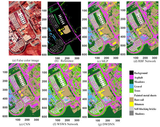
Figure 6.
Classification results of the Pavia University dataset (the instances without class information were also predicted). (a) False color image, (b) reference image, (c) MLP, (d) RBF Network, (e) CNN, (f) WSWS Network, and (g) DWDNN.
The classification results for the Salinas dataset are shown in Table 5 and Figure 7. The proposed DWDNN had the best classification results compared with the other methods, and the OA, AA, and Kappa coefficient were 99.76%, 99.73%, and 99.73%, respectively. The test accuracy for each class in the table represents how many samples can be classified correctly among the total number of samples in the corresponding class. The instances without class information were predicted as shown in Figure 7. The proposed DWDNN had smoother predicted results than the compared methods, which can be seen from the predicted classes of grapes-untrained with purple color and vineyard-untrained with dark yellow color in Figure 7g.
Table 5.
Classification results of different methods on the Salinas dataset.
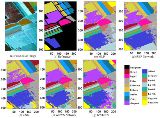
Figure 7.
Classification results of the Salinas dataset (the instances without class information were also predicted). (a) false color image, (b) Reference image, (c) MLP, (d) RBF Network, (e) CNN, (f) WSWS Network, and (g) DWDNN.
5. Discussion
5.1. Visualization of the Extracted Features from the DWDNN
In this discussion, the extracted high-level features are visualized to show that the proposed DWDNN can extract different features effectively. Therefore, it can have a good performance on the HSI classification task.
For the Botswana dataset, the proportion for training and validation was 0.2, and 0.2. The basic parameter group of each single EWSWS network had: 4 EWSWS layers and 12, 71, 80, and 40 for the stride number, window size, number of transform kernels, and subsampling number for the first EWSWS layer; 400, 0.1 of the length of the current input vector, 40, and 20 for the stride number, window size, number of transform kernels, and subsampling number for the second EWSWS layer; 60, 0.7 of the length of the current input vector, 40, and 20 for the stride number, window size, number of transform kernels, and subsampling number for the third EWSWS layer; and 2, 0.5 of the length of the current input vector, 20, and 10 for the stride number, window size, number of transform kernels, and subsampling number for the fourth EWSWS layer, respectively.
For the Pavia University dataset, the proportion of training and validation was 0.2 and 0.2. The basic parameter group of each single EWSWS network was: 4 EWSWS layers and 2, 5, 100, 50 for the stride number, window size, number of transform kernels, and subsampling number for the first EWSWS layer; 320, 0.1 of the length of the current input vector, 100, and 50 for the stride number, window size, number of transform kernels, and subsampling number for the second EWSWS layer; 40, 0.2 of the length of the current input vector, 32, and 16 for the stride number, window size, number of transform kernels, and subsampling number for the third EWSWS layer; and 12, 0.3 of the length of the current input vector, 12, and 6 for the stride number, window size, number of transform kernels, and subsampling number for the fourth EWSWS layer, respectively.For the Salinas datasets, the settings were the same as in Table 2.
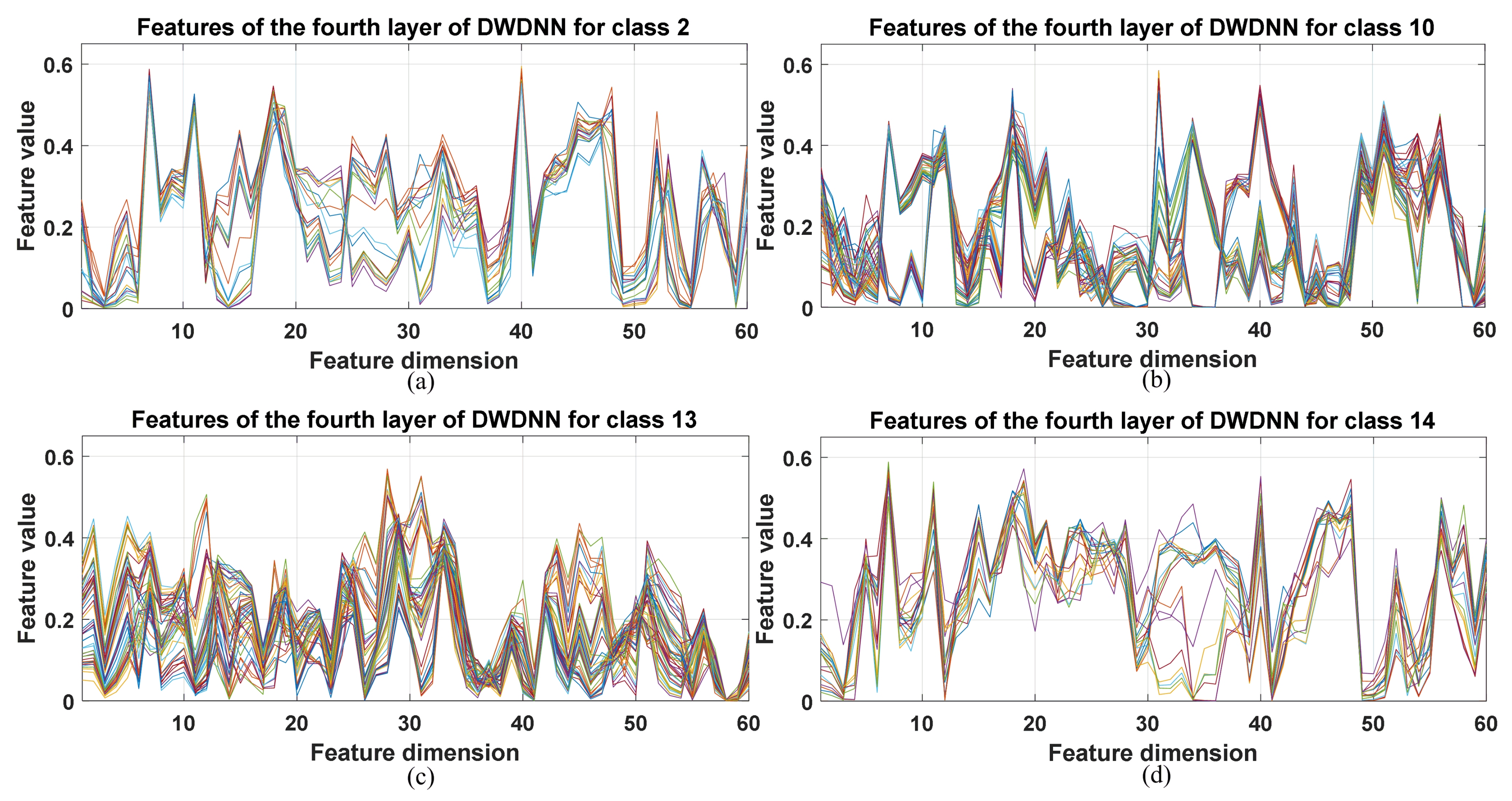
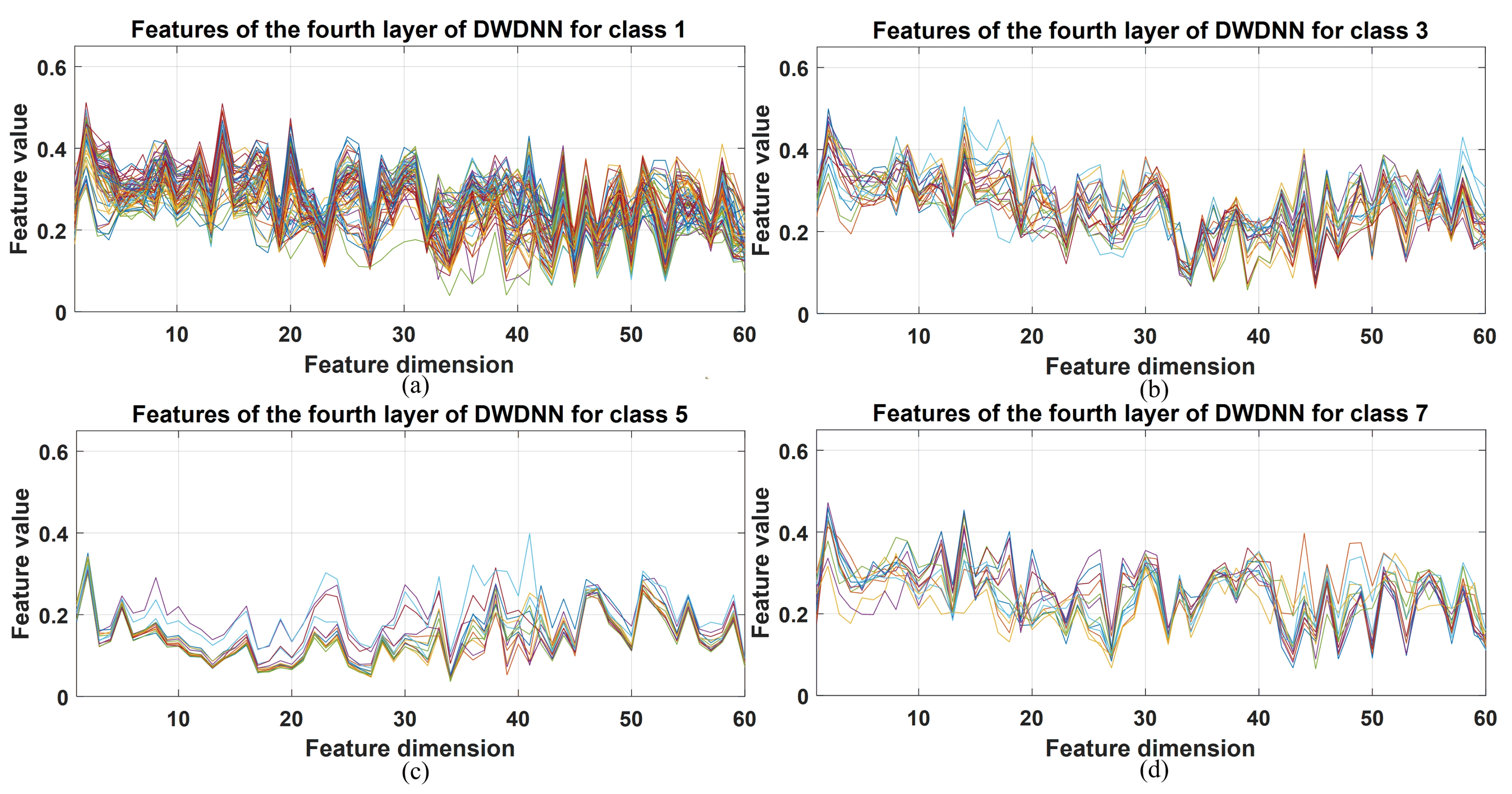
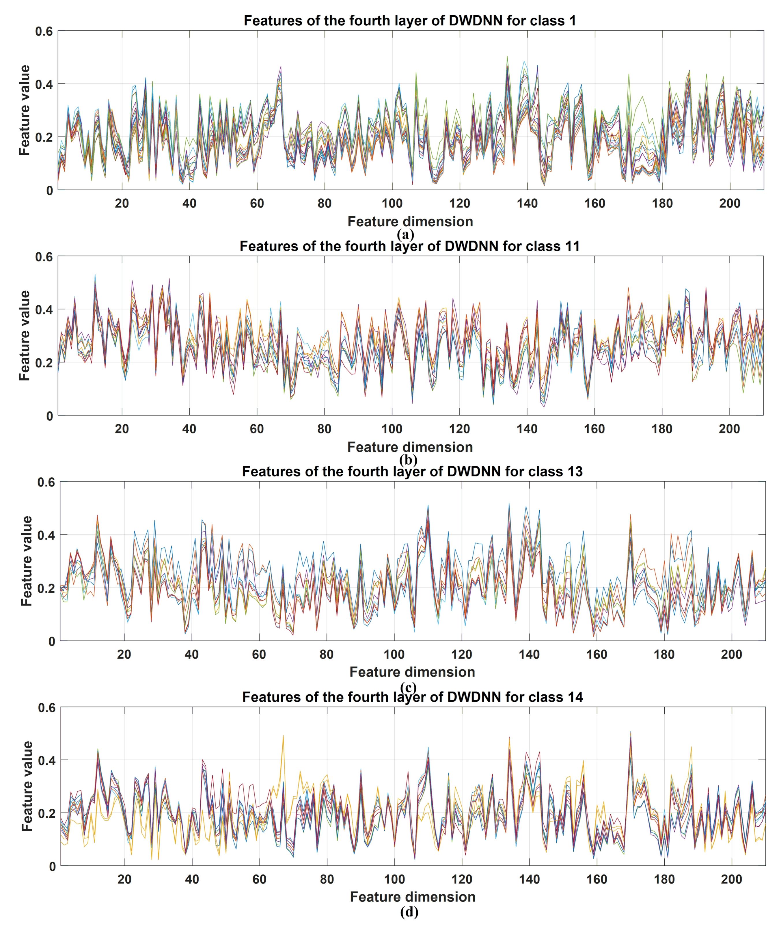
The DWDNN was composed of multiple EWSWS networks, and each EWSWS network had multiple layers to extract features from the low level to the high level. The extracted features of the DWDNN with the hyperspectral datasets are shown in Figure 8, Figure 9 and Figure 10. These extracted features were from the training samples and combined in a cascade from the fourth layer of the transform kernels in the DWDNN. Each curve in the figures represents an extracted feature vector from the training instances with the same classes. For the Botswana dataset, the extracted features from Classes 2, 10, 13, and 14 are shown. All the training instances of the same class were stacked together. It is observed in Figure 8 that the extracted features of the same class have very similar curves. Classes 10 and 13 have more training samples, but they still have very similar feature curves. For Pavia University, the extracted features from Classes 1, 3, 5, and 7 are shown. There were 0.1 of the total number of the training instances of the same class stacked together. It is observed in Figure 9 that all the classes have very similar feature curves. Class 1 has more training samples, but it still has similar feature curves for these samples. For Salinas, the extracted features from Classes 1, 11, 13, and 14 are shown. There were 0.1 of the total number of the training instances of the same class stacked together. It is observed in Figure 10 that all the classes have very similar feature curves. Because 210 features were extracted and shown, these feature curves are denser compared with the other two datasets.
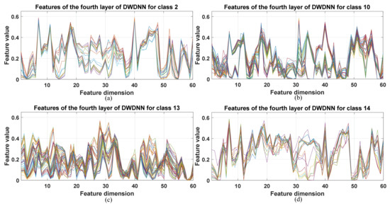
Figure 8.
Stacked extracted features of the training instances from the last transform kernel layers of the DWDNN (10 EWSWS networks) with the Botswana dataset. (a) Extracted features for class 2. (b) Extracted features for class 10. (c) Extracted features for class 13. (d) Extracted features for class 14.

Figure 9.
Stacked extracted features of the training instances from the last transform kernel layers of the DWDNN (10 EWSWS networks) with the Pavia University dataset. (a) Extracted features for class 1. (b) Extracted features for class 3. (c) Extracted features for class 5. (d) Extracted features for class 7.
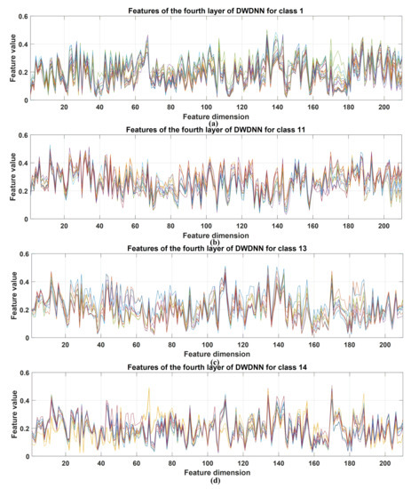
Figure 10.
Stacked extracted features of the training instances from the last transform kernel layers of the DWDNN (10 EWSWS networks) with the Salinas dataset. (a) Extracted features for class 1. (b) Extracted features for class 11. (c) Extracted features for class 13. (d) Extracted features for class 14.
It is observed from all the figures with the three datasets that different classes have different feature curves, and the instances in the same class have similar feature curves. This demonstrated that the proposed DWDNN can learn features effectively with the HSI data.
5.2. Smooth Fine-grained Learning with Different Numbers of EWSWS Networks
In this part, the experimental setting of the Botswana data was the same as in the previous discussion.
For the Pavia University and Salinas datasets, the settings were the same as in Table 2. The main advantage of the DWDNN is that it can learn smoothly with fine-grained hyperparameter settings. That is because the features can be learned in both the deep and wide directions iteratively. The DWDNN was composed of a number of EWSWS Nets, and the training can start from an EWSWS network with a basic group of parameters, then it can learn incrementally with the succeeding EWSWS networks one after the other. Therefore, the DWDNN with the proper architectural complexity can be obtained without overfitting.
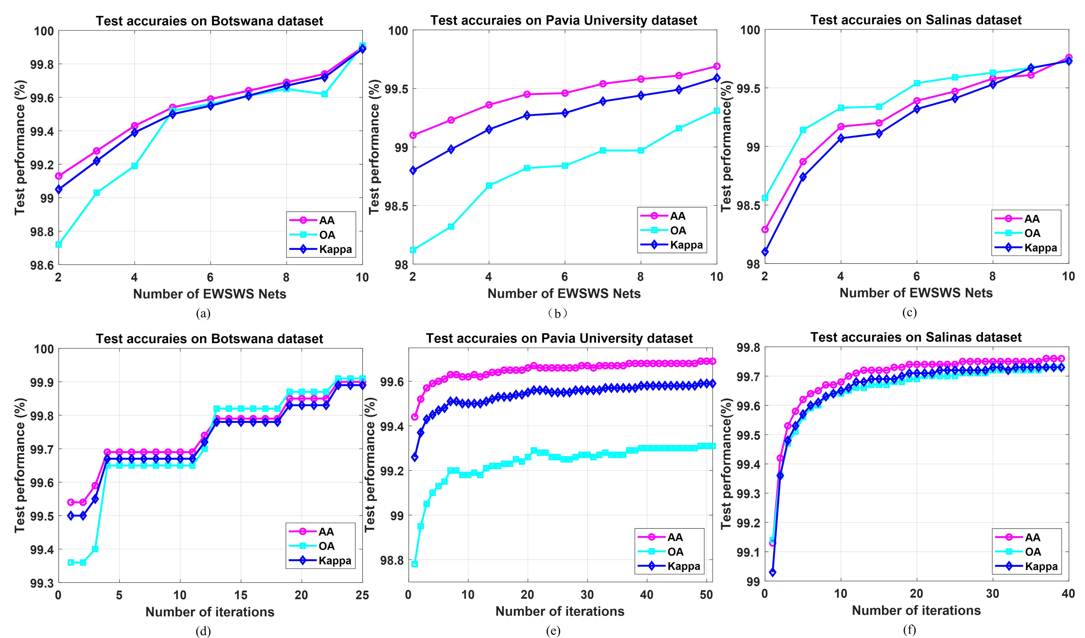
It is observed in Table 6, Table 7 and Table 8 that the performance can be improved smoothly as the number of EWSWS networks increases. The testing performance of the iteration process with the DWDNN including 10 EWSWS networks is shown in Figure 11. During the iterations, the testing performance improved steadily. The iterations were stopped by the validation process. In Table 6, Table 7 and Table 8, the testing accuracies started increasing above 98% as the number of EWSWS networks increased. The number of EWSWS networks can actually be reduced to reach the desired and sufficient testing performance. It is also observed in Figure 11 that the iteration can start from a point with good performance to reduce the number of iterations.
Table 6.
Classification results with different numbers of EWSWS networks with the Botswana dataset.
Table 7.
Classification results with different numbers of EWSWS networks with the Pavia University dataset.
Table 8.
Classification results with different numbers of EWSWS networks with the Salinas dataset.
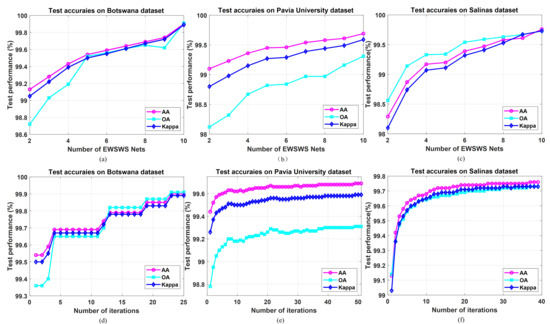
Figure 11.
Classification results of the DWDNN with different numbers of EWSWS networks and different iterations (10 EWSWS networks). (a–c) Classification results of the DWDNN with different numbers of EWSWS networks. (d–f) Classification results of the DWDNN with different iterations (10 EWSWS networks).
5.3. Running Time Analysis
The proposed method was extended in both the wide and deep direction. The number of EWSWS networks, the strides for the sliding windows, and the subsampling ratios at each EWSWS layer can be used to balance the performance and the computational load. The running time including the training and testing were compared with different methods on the Botswana dataset for further discussion. The parameter settings were the same as in Section 4. The results are shown in Table 9. Compared with the classical machine learning models MLP and RBF and the recently proposed WSWS network, the proposed DWDNN has longer training time, but it still has a good testing time. That is because the DWDNN was composed of 10 EWSWS networks, and it needed a bit more time to train the model iteratively. During the testing process, it can compute quickly because the parameters of the DWDNN were reduced greatly using the measures such as the strides for the sliding windows and subsampling for the transform kernels. The proposed DWDNN had both a shorter training and testing time compared to the CNN.
Table 9.
Running time analysis with the Botswana dataset.
6. Conclusions
Recently, deep learning has been used effectively in hyperspectral image classification. However, it is hard to take full advantage of deep learning networks because of the limited training instances with hyperspectral remote sensing scenes. That is because the acquisition of hyperspectral remote sensing images is usually expensive. How to overcome overfitting as a result becomes an important issue for hyperspectral image classification with deep learning. In this paper, we proposed a dynamic wide and deep neural network (DWDNN) for hyperspectral image classification. It was composed of multiple efficient wide sliding windows and subsampling (EWSWS) networks, which can be generated dynamically according to the complexity of the learning tasks. Therefore, a learning architecture with proper complexity can be generated to overcome overfitting. Each EWSWS network was extended both in the wide and deep directions with the transform kernels as the hidden units. The fine-grained features can be learned smoothly and effectively because the sliding windows with strides and subsampling were designed to both reduce the dimension of the features and retain the important features. In the DWDNN, only the weights of the fully connected layers are computed using iterative least squares, which makes it easy to train the DWDNN. The proposed method was evaluated with the Botswana, Pavia University, and Salinas HSI datasets. The experimental results of the proposed DWDNN had the best performance among the compared methods including the classical machine learning methods and some recently proposed deep learning models for hyperspectral image classification. The limitation of the proposed method is how to extract two-dimensional spatial features effectively in images as the CNN does. This is because the image patches were flattened into vectors, and one-dimensional features were extracted in the sliding windows through the EWSWS layers, which may weaken the spatial structure of the HSIs. This can be studied in the future by using two-dimensional transform kernels directly for HSIs.
Author Contributions
All the authors made significant contributions to this work. All authors contributed to the methodology validation and results analysis and reviewed the manuscript. Conceptualization, O.K.E. and J.X.; methodology, J.X. and M.C.; software and experiments, J.X. and M.C.; validation, W.Z., J.G. and T.W.; writing, original draft preparation, J.X.; funding acquisition, Z.L., C.Z. and W.Z. All authors read and agreed to the published version of the manuscript.
Funding
This work was supported in part by the National Key R&D Program of China under Grant 2018YFC1504805; in part by the National Natural Science Foundation of China under Grants 61806022, 41941019, and 41874005; in part by the Fundamental Research Funds for the Central Universities, 300102269103, 300102269304, 300102260301, 300102261404, and 300102120201; in part by Fund No.19-163-00-KX-002-030-01; in part by the Key Research and Development Program of Shaanxi (Grant No. 2021NY-170); in part by the Special Project of Forestry Science and Technology Innovation Plan in Shaanxi Province SXLK2021-0225; and in part by the China Scholarship Council (CSC) under Scholarship 201404910404.
Acknowledgments
The authors are grateful to the Editor and reviewers for their constructive comments, which significantly improved this work.
Conflicts of Interest
The authors declare no conflict of interest.
Abbreviations
The following abbreviations are used in this manuscript:
| HSI | Hyperspectral image |
| DWDNN | Dynamic wide and deep neural network |
| EWSWS | Wide sliding window and subsampling |
| MLR | Multinomial logistic regression |
| SVM | Support vector machine |
| MLP | Multilayer perceptron |
| RF | Random forest |
| CNN | Convolutional neural network |
| DSVM | Deep support vector machine |
| FCN | Fully convolutional network |
| EWC | Elastic weight consolidation |
| IMM | Incremental moment matching |
| PSHNN | Parallel, self-organizing, hierarchical neural network |
| PCNN | Parallel consensual neural network |
| CDL | Conditional deep learning |
| SCNs | Stochastic configuration network |
| PCA | Principal component analysis |
| OA | Overall accuracy |
| AA | Average accuracy |
| DRNN | Deep recurrent neural network |
| WSWS | Wide sliding window and subsampling |
| SMSB | Sparse modeling of spectral block |
References
- Li, W.; Wu, G.; Zhang, F.; Du, Q. Hyperspectral image classification using deep pixel-pair features. IEEE Trans. Geosci. Remote Sens. 2016, 55, 844–853. [Google Scholar] [CrossRef]
- Böhning, D. Multinomial logistic regression algorithm. Ann. Inst. Stat. Math. 1992, 44, 197–200. [Google Scholar] [CrossRef]
- Tarabalka, Y.; Fauvel, M.; Chanussot, J.; Benediktsson, J.A. SVM-and MRF-based method for accurate classification of hyperspectral images. IEEE Geosci. Remote Sens. Lett. 2010, 7, 736–740. [Google Scholar] [CrossRef] [Green Version]
- Safavian, S.R.; Landgrebe, D. A survey of decision tree classifier methodology. IEEE Trans. Syst. Man Cybern. 1991, 21, 660–674. [Google Scholar] [CrossRef] [Green Version]
- Xi, J.; Ersoy, O.K.; Fang, J.; Wu, T.; Wei, X.; Zhao, C. Parallel Multistage Wide Neural Network; Technical Reports, 757; Department of Electrical and Computer Engineering, Purdue University: West Lafayette, Indiana, 2020. [Google Scholar]
- Li, J.; Bioucas-Dias, J.M.; Plaza, A. Semisupervised hyperspectral image classification using soft sparse multinomial logistic regression. IEEE Geosci. Remote Sens. Lett. 2012, 10, 318–322. [Google Scholar]
- Wu, Z.; Wang, Q.; Plaza, A.; Li, J.; Liu, J.; Wei, Z. Parallel implementation of sparse representation classifiers for hyperspectral imagery on GPUs. IEEE J. Sel. Top. Appl. Earth Obs. Remote Sens. 2015, 8, 2912–2925. [Google Scholar] [CrossRef]
- Lee, H.; Kwon, H. Going deeper with contextual CNN for hyperspectral image classification. IEEE Trans. Image Process. 2017, 26, 4843–4855. [Google Scholar] [CrossRef] [PubMed] [Green Version]
- Mei, S.; Ji, J.; Hou, J.; Li, X.; Du, Q. Learning sensor-specific spatial-spectral features of hyperspectral images via convolutional neural networks. IEEE Trans. Geosci. Remote Sens. 2017, 55, 4520–4533. [Google Scholar] [CrossRef]
- Gao, Q.; Lim, S.; Jia, X. Hyperspectral image classification using convolutional neural networks and multiple feature learning. Remote Sens. 2018, 10, 299. [Google Scholar] [CrossRef] [Green Version]
- Wang, W.; Dou, S.; Jiang, Z.; Sun, L. A fast dense spectral–spatial convolution network framework for hyperspectral images classification. Remote Sens. 2018, 10, 1068. [Google Scholar] [CrossRef] [Green Version]
- Paoletti, M.; Haut, J.; Plaza, J.; Plaza, A. A new deep convolutional neural network for fast hyperspectral image classification. ISPRS J. Photogramm. Remote Sens. 2018, 145, 120–147. [Google Scholar] [CrossRef]
- Zhang, M.; Li, W.; Du, Q. Diverse region-based CNN for hyperspectral image classification. IEEE Trans. Image Process. 2018, 27, 2623–2634. [Google Scholar] [CrossRef]
- Cheng, G.; Li, Z.; Han, J.; Yao, X.; Guo, L. Exploring hierarchical convolutional features for hyperspectral image classification. IEEE Trans. Geosci. Remote Sens. 2018, 56, 6712–6722. [Google Scholar] [CrossRef]
- Gong, Z.; Zhong, P.; Yu, Y.; Hu, W.; Li, S. A CNN With Multiscale Convolution and Diversified Metric for Hyperspectral Image Classification. IEEE Trans. Geosci. Remote Sens. 2019, 57, 3599–3618. [Google Scholar] [CrossRef]
- Hamida, A.B.; Benoit, A.; Lambert, P.; Amar, C.B. 3D deep learning approach for remote sensing image classification. IEEE Trans. Geosci. Remote Sens. 2018, 56, 4420–4434. [Google Scholar] [CrossRef] [Green Version]
- Zheng, J.; Feng, Y.; Bai, C.; Zhang, J. Hyperspectral Image Classification Using Mixed Convolutions and Covariance Pooling. IEEE Trans. Geosci. Remote Sens. 2020, 59, 522–534. [Google Scholar] [CrossRef]
- Roy, S.K.; Krishna, G.; Dubey, S.R.; Chaudhuri, B.B. HybridSN: Exploring 3D–2D CNN feature hierarchy for hyperspectral image classification. IEEE Geosci. Remote Sens. Lett. 2019, 17, 277–281. [Google Scholar] [CrossRef] [Green Version]
- Haut, J.M.; Paoletti, M.E.; Plaza, J.; Li, J.; Plaza, A. Active Learning With Convolutional Neural Networks for Hyperspectral Image Classification Using a New Bayesian Approach. IEEE Trans. Geosci. Remote Sens. 2018, 56, 6440–6461. [Google Scholar] [CrossRef]
- Cao, X.; Yao, J.; Xu, Z.; Meng, D. Hyperspectral image classification with convolutional neural network and active learning. IEEE Trans. Geosci. Remote Sens. 2020, 58, 4604–4616. [Google Scholar] [CrossRef]
- Tang, X.; Meng, F.; Zhang, X.; Cheung, Y.; Ma, J.; Liu, F.; Jiao, L. Hyperspectral Image Classification Based on 3D Octave Convolution With Spatial-Spectral Attention Network. IEEE Trans. Geosci. Remote Sens. 2020, 59, 1–18. [Google Scholar] [CrossRef]
- Masarczyk, W.; Głomb, P.; Grabowski, B.; Ostaszewski, M. Effective Training of Deep Convolutional Neural Networks for Hyperspectral Image Classification through Artificial Labeling. Remote Sens. 2020, 12, 2653. [Google Scholar] [CrossRef]
- Xie, F.; Gao, Q.; Jin, C.; Zhao, F. Hyperspectral image classification based on superpixel pooling convolutional neural network with transfer learning. Remote Sens. 2021, 13, 930. [Google Scholar] [CrossRef]
- Cui, Y.; Xia, J.; Wang, Z.; Gao, S.; Wang, L. Lightweight Spectral-Spatial Attention Network for Hyperspectral Image Classification. IEEE Trans. Geosci. Remote Sens. 2021, 1–14. [Google Scholar] [CrossRef]
- Yuan, Y.; Wang, C.; Jiang, Z. Proxy-Based Deep Learning Framework for Spectral-Spatial Hyperspectral Image Classification: Efficient and Robust. IEEE Trans. Geosci. Remote Sens. 2021, 1–15. [Google Scholar] [CrossRef]
- Mou, L.; Ghamisi, P.; Zhu, X.X. Deep recurrent neural networks for hyperspectral image classification. IEEE Trans. Geosci. Remote Sens. 2017, 55, 3639–3655. [Google Scholar] [CrossRef] [Green Version]
- Okwuashi, O.; Ndehedehe, C.E. Deep support vector machine for hyperspectral image classification. Pattern Recognit. 2020, 103, 107298. [Google Scholar] [CrossRef]
- Worrall, D.E.; Garbin, S.J.; Turmukhambetov, D.; Brostow, G.J. Harmonic networks: Deep translation and rotation equivariance. In Proceedings of the IEEE Conference on Computer Vision and Pattern Recognition, Honolulu, HI, USA, 21–26 July 2017; pp. 5028–5037. [Google Scholar]
- Liu, C.; Li, J.; He, L.; Plaza, A.; Li, S.; Li, B. Naive Gabor Networks for Hyperspectral Image Classification. IEEE Trans. Neural Netw. Learn. Syst. 2020, 103, 376–390. [Google Scholar] [CrossRef]
- Cao, F.; Guo, W. Cascaded dual-scale crossover network for hyperspectral image classification. Knowl. Based Syst. 2020, 189, 105122. [Google Scholar] [CrossRef]
- Li, H.C.; Li, S.S.; Hu, W.S.; Feng, J.H.; Sun, W.W.; Du, Q. Recurrent Feedback Convolutional Neural Network for Hyperspectral Image Classification. IEEE Geosci. Remote Sens. Lett. 2021, 1–5. [Google Scholar] [CrossRef]
- Roy, S.K.; Haut, J.M.; Paoletti, M.E.; Dubey, S.R.; Plaza, A. Generative Adversarial Minority Oversampling for Spectral-Spatial Hyperspectral Image Classification. IEEE Trans. Geosci. Remote Sens. 2021, 1–15. [Google Scholar] [CrossRef]
- Parisi, G.I.; Kemker, R.; Part, J.L.; Kanan, C.; Wermter, S. Continual lifelong learning with neural networks: A review. Neural Netw. 2019, 113, 54–71. [Google Scholar] [CrossRef]
- Kirkpatrick, J.; Pascanu, R.; Rabinowitz, N.; Veness, J.; Desjardins, G.; Rusu, A.A.; Milan, K.; Quan, J.; Ramalho, T.; Grabska-Barwinska, A.; et al. Overcoming catastrophic forgetting in neural networks. Proc. Natl. Acad. Sci. USA 2017, 114, 3521–3526. [Google Scholar] [CrossRef] [Green Version]
- Lee, S.W.; Kim, J.H.; Jun, J.; Ha, J.W.; Zhang, B.T. Overcoming catastrophic forgetting by incremental moment matching. In Advances in Neural Information Processing Systems; MIT Press: Cambridge, MA, USA, 2017; pp. 4652–4662. [Google Scholar]
- Ersoy, O.K.; Hong, D. Parallel, self-organizing, hierarchical neural networks. IEEE Trans. Neural Netw. 1990, 1, 167–178. [Google Scholar] [CrossRef] [Green Version]
- Benediktsson, J.A.; Sveinsson, J.R.; Ersoy, O.K.; Swain, P.H. Parallel consensual neural networks. IEEE Trans. Neural Netw. 1997, 8, 54–64. [Google Scholar] [CrossRef] [Green Version]
- Venkataramani, S.; Raghunathan, A.; Liu, J.; Shoaib, M. Scalable-effort classifiers for energy-efficient machine learning. In Proceedings of the 52nd Annual Design Automation Conference, San Francisco, CA, USA, 8–12 June 2015; ACM: New York, NY, USA, 2015; p. 67. [Google Scholar]
- Panda, P.; Venkataramani, S.; Sengupta, A.; Raghunathan, A.; Roy, K. Energy-Efficient Object Detection Using Semantic Decomposition. IEEE Trans. Very Large Scale Integr. (VLSI) Syst. 2017, 25, 2673–2677. [Google Scholar] [CrossRef]
- Roy, D.; Panda, P.; Roy, K. Tree-CNN: A Deep Convolutional Neural Network for Lifelong Learning. arXiv 2018, arXiv:1802.05800. [Google Scholar]
- Panda, P.; Sengupta, A.; Roy, K. Conditional Deep Learning for energy-efficient and enhanced pattern recognition. In Proceedings of the 2016 Design, Automation Test in Europe Conference Exhibition (DATE), Dresden, Germany, 14–18 March 2016; pp. 475–480. [Google Scholar]
- Wang, D.; Li, M. Stochastic Configuration Networks: Fundamentals and Algorithms. IEEE Trans. Cybern. 2017, 47, 3466–3479. [Google Scholar] [CrossRef] [Green Version]
- Kwon, H.; Lee, J. AdvGuard: Fortifying Deep Neural Networks against Optimized Adversarial Example Attack. IEEE Access 2020. [Google Scholar] [CrossRef]
- Kwon, H.; Yoon, H.; Park, K.W. Multi-targeted backdoor: Indentifying backdoor attack for multiple deep neural networks. IEICE Trans. Inf. Syst. 2020, 103, 883–887. [Google Scholar] [CrossRef]
- Neyshabur, B.; Li, Z.; Bhojanapalli, S.; LeCun, Y.; Srebro, N. The role of over-parametrization in generalization of neural networks. In Proceedings of the International Conference on Learning Representations, New Orleans, LA, USA, 6–9 May 2019. [Google Scholar]
- Lee, J.; Xiao, L.; Schoenholz, S.S.; Bahri, Y.; Sohl-Dickstein, J.; Pennington, J. Wide neural networks of any depth evolve as linear models under gradient descent. arXiv 2019, arXiv:1902.06720. [Google Scholar]
- Cheng, H.T.; Koc, L.; Harmsen, J.; Shaked, T.; Chandra, T.; Aradhye, H.; Anderson, G.; Corrado, G.; Chai, W.; Ispir, M.; et al. Wide & deep learning for recommender systems. In Proceedings of the 1st Workshop on Deep Learning for Recommender Systems, Boston, MA, USA, 15 September 2016; ACM: New York, NY, USA, 2016; pp. 7–10. [Google Scholar]
- Jahan, F.; Zhou, J.; Awrangjeb, M.; Gao, Y. Fusion of hyperspectral and LiDAR data using discriminant correlation analysis for land cover classification. IEEE J. Sel. Top. Appl. Earth Obs. Remote Sens. 2018, 11, 3905–3917. [Google Scholar] [CrossRef] [Green Version]
- Jahan, F.; Zhou, J.; Awrangjeb, M.; Gao, Y. Inverse Coefficient of Variation Feature and Multilevel Fusion Technique for Hyperspectral and LiDAR Data Classification. IEEE J. Sel. Top. Appl. Earth Obs. Remote Sens. 2020, 13, 367–381. [Google Scholar] [CrossRef] [Green Version]
- Xi, J.; Ersoy, O.K.; Fang, J.; Cong, M.; Wu, T.; Zhao, C.; Li, Z. Wide Sliding Window and Subsampling Network for Hyperspectral Image Classification. Remote Sens. 2021, 13, 1290. [Google Scholar] [CrossRef]
- Aghagolzadeh, S.; Ersoy, O.K. Optimal adaptive multistage image transform coding. IEEE Trans. Circuits Syst. Video Technol. 1991, 1, 308–317. [Google Scholar] [CrossRef] [Green Version]
- Xi, J.; Ersoy, O.K.; Fang, J.; Cong, M.; Wei, X.; Wu, T. Scalable Wide Neural Network: A Parallel, Incremental Learning Model Using Splitting Iterative Least Squares. IEEE Access 2021, 9, 50767–50781. [Google Scholar] [CrossRef]
- Hyperspectral Remote Sensing Scenes. Available online: http://www.ehu.eus/ccwintco/index.php?title=Hyperspectral_Remote_Sensing_Scenes#Indian_Pines (accessed on 25 March 2021).
- Melgani, F.; Bruzzone, L. Classification of hyperspectral remote sensing images with support vector machines. IEEE Trans. Geosci. Remote Sens. 2004, 42, 1778–1790. [Google Scholar] [CrossRef] [Green Version]
- Chen, Y.; Jiang, H.; Li, C.; Jia, X.; Ghamisi, P. Deep feature extraction and classification of hyperspectral images based on convolutional neural networks. IEEE Trans. Geosci. Remote Sens. 2016, 54, 6232–6251. [Google Scholar] [CrossRef] [Green Version]
- Azar, S.G.; Meshgini, S.; Rezaii, T.Y.; Beheshti, S. Hyperspectral image classification based on sparse modeling of spectral blocks. Neurocomputing 2020, 407, 12–23. [Google Scholar] [CrossRef]


Publisher’s Note: MDPI stays neutral with regard to jurisdictional claims in published maps and institutional affiliations. |
© 2021 by the authors. Licensee MDPI, Basel, Switzerland. This article is an open access article distributed under the terms and conditions of the Creative Commons Attribution (CC BY) license (https://creativecommons.org/licenses/by/4.0/).