Article

MAMOTH: An Earth Observational Data-Driven Model for Mosquitoes Abundance Prediction

by
Argyro Tsantalidou
1,*,†,
Elisavet Parselia
2,†,
George Arvanitakis
1,2,
Katerina Kyratzi
2,
Sandra Gewehr
3,
Athena Vakali
1 and
Charalampos Kontoes
2
1
Informatics School, Aristotle University of Thessaloniki, 54121 Thessaloniki, Greece
2
National Observatory of Athens, IAASARS, BEYOND Center for EO Research and Satellite Remote Sensing, 11523 Athens, Greece
3
Ecodevelopment S.A., 57010 Thessaloniki, Greece
*
Author to whom correspondence should be addressed.
These authors contributed equally to this work.
Remote Sens. 2021, 13(13), 2557; https://doi.org/10.3390/rs13132557
Submission received: 31 March 2021 / Revised: 8 June 2021 / Accepted: 25 June 2021 / Published: 30 June 2021

Abstract

:
Mosquito-Borne Diseases (MBDs) are known to be more prevalent in the tropics, and yet, in the last two decades, they are spreading to many other countries, especially in Europe. The set (volume) of environmental, meteorological and other spatio-temporally variable parameters affecting mosquito abundance makes the modeling and prediction tasks quite challenging. Up to now, mosquito abundance prediction problems were addressed with ad-hoc area-specific and genus-tailored approaches. We propose and develop MAMOTH, a generic and accurate Machine Learning model that predicts mosquito abundances for the upcoming period (the Mean Absolute Error of the predictions do not deviate more than 14 % ). The designed model relies on satellite Earth Observation and other in-situ geo-spatial data to tackle the problem. MAMOTH is not site- nor mosquito genus-dependent; thus, it can be easily replicated and applied to multiple cases without any special parametrization. The model was applied to different mosquito genus and species Culex spp. as potential vectors for West Nile Virus, Anopheles spp. for Malaria and Aedes albopictus for Zika/Chikungunya/Dengue) and in different areas of interest (Italy, Serbia, France, Germany). The results show that the model performs accurately and consistently for all case studies. Additionally, the evaluation of different cases, with the model using the same principles, provides an opportunity for multi-case and multi-scope comparative studies.

1. Introduction

Mosquito-Borne Diseases (MBDs) are infectious diseases transmitted by mosquitoes and are responsible for morbidity and mortality in humans. They are part of the Vector-Borne Diseases (VBDs), which account for more than 17% of all infectious diseases and cause more than 700,000 deaths annually [1]. Climate change, travel, and trade can influence the seasonal and geographical spread of mosquitoes and, thus, the transmission of pathogens. Although MDBs can be found in many areas around the world, tropical and subtropical are the ones suffering the most, while different mosquito species carry different pathogens causing various types of MBDs [2]. MBDs, such as West Nile Virus (WNV) transmitted by mosquitoes of the Culex genus, Malaria transmitted by mosquitoes of the Anopheles genus, and Chikungunya, Dengue, and Zika transmitted by Aedes albopictus in Europe have posed challenges to national public health authorities in the European region [3].
It is a widely mistaken belief that the MBDs are only affecting the developing countries; Europe has experienced many cases of MBDs outbreaks in the last two decades. The year 2010 was one with large outbreaks of West Nile Virus in Greece and Russia, having 262 and 419 human cases, respectively, and a total of 1016 cases across all Europe [4]. WNV human infections have sharply increased in 2018 compared to the previous years. According to ECDC, in 2019, 615 cases were reported in Italy, 315 cases in Greece, and 277 cases in Romania. In total, 1548 cases were locally acquired, and 166 deaths were reported. Additionally, 415 WNV cases were recorded in Serbia with 35 deaths [5]. Furthermore, according to ECDC, the number of confirmed Malaria cases reported in the EU from 2008 to 2012 ranged between approximately 5000 and 7000 [6], whereas, in 2018, it reached almost 8500 [7]. All the evidence show that there is a need for preventive actions to mitigate the problem.
A lot of earlier research focuses on predicting the upcoming MBDs risk in order to support decision-making by successfully designing preventive and mosquito control measures in time and space. The state of the art can be divided into two main directions, one that aims at predicting the upcoming human cases risk (epidemiological approach) and the other that aims at predicting the mosquito populations (entomological approach). As expected, the probability of human infection and the mosquito population in a given area are strongly dependent variables [8].
A number of issues have posed difficulties in mosquito population monitoring and forecasting up to date. The lack of well structured, consistent and reliable environmental, landscape, and ecosystem data, and their change over time that makes them hard to collect, are some of the most important barriers. The necessary placement of in-situ equipment for environmental data collection is limiting the study area either because of the high cost of operation and maintenance or the inaccessibility of an area. Different spatio-temporal resolutions, re-sampling, and filtering techniques in limited areas increase significantly the complexity of comparative studies. However, the advent and plethora of satellite Earth Observation (EO) Big Data from multiple sensors (e.g., Sentinel, Landsat, TERRA/AQUA (MODIS), etc.), which allow frequent revisit times and larger coverage, enable enhanced earth monitoring at global level and provide vast amounts of data that are consistent and accessible via open data platforms [9]. In addition, the revolution in data science and machine learning (ML) algorithms provides many opportunities for accurate and reliable data-driven solutions to the problem [10].

1.1. Related Work

There are approaches that evaluate analytical dynamic models to predict the upcoming human infections or the mosquito populations. In Reference [11], researchers attempted to identify conditions conducive to a WNV outbreak in Greece using an epidemiological model of differential equations. Other approaches use environmental/meteorological data and simple statistical approaches that attempt to identify the conditions favoring the spread of MBDs and can be used for mitigation measures. Authors in Reference [12] concluded through observational analysis that a rapid increase in temperature is associated with an increase in human WNV cases in the West Virginia area of the United States. Authors in Reference [13] perform a two step cluster analysis to classify areas in Greece into low, medium, and high risk for the spread of WNV virus. In Reference [14], a statistical analysis was performed for Morocco, and it was found that extreme rainfall and high Normalized Difference Vegetation Index (NDVI) values are the factors that contribute to WNV amplification.
In recent years, due to the progress in the field of ML, a lot of valuable studies that combine remote sensing data with ML techniques have been proposed. The authors in Reference [15] proposed a novel machine learning method for classification of high-spectral images based on the estimated spectral profiles per pixel, providing a promising segmentation of materials lying over or beneath the Earth’s surface, while the authors in Reference [16] proposed the use of deep learning classifiers which combine different sources of information and extract high level features, able to achieve better classification results with remote sensing images. More detailed information can be found in Reference [17]. This overall progress in the field of remote sensing offered more sophisticated data-driven models to help control MBDs. A lot of algorithms have been used in different areas with various features and techniques. Ref. [18,19] used Support Vector Machine (SVM) to predict Malaria and Dengue cases in India and China, respectively. Both were based on epidemiological and environmental data. General additive models are also a popular method for predicting WNV in the Great Plains of the United States [20] and Malaria in Kenya [21]. The K-Nearest Neighbors (KNN) algorithm was utilized to estimate the weekly mosquito population in northwestern Argentina [22]. Authors in Reference [23], after training many decision trees to predict WNV incidence across different areas of the United States over the years, concluded that there is not a single model fitting one area over the years, but rather a model fitting many areas in a specific year is more feasible.
However, in all cases studied, limited selected environmental data were included, such as temperature and precipitation, which were used as predictors, along with other kinds of features depending on each case study. Each work presents a model or an architecture that focuses on a specific mosquito genus/disease and area of interest, so all of these approaches are not directly comparable and are site-specific and genus-specific. These limitations hinder the scalability and generic applicability of the developed approaches. In this view arises the need for a generic integrated, scalable, and reliable Early Warning System (EWS). The idea of the prototype EYWA system, developed under the flag of the EuroGEO Action Group for Epidemics, came to overcome several of the aforementioned limitations, thus delivering a scalable and robust solution, as shown in the following sections.

1.2. Our Approach

This work is motivated by the lack of a widely accepted, standardized, and generic solution for the problem of mosquito abundance predictions. Taking advantage of the recent progress in the ML domain, and integrating multi-source EO data to extract environmental, landscape, and ecosystem related information in a consistent, uniform, and reliable way, we focus on designing an early warning predictor of the upcoming mosquito population. Our goal is to design a location and genus agnostic model out of a generic and adaptive framework. This gave birth to MAMOTH (Mosquitoes Abundance Prediction Model autO-calibrated from features pleTHora), presented hereinafter, a generic framework that requires no human intervention in selection of the features or model’s hyper-parameters tuning. In this paper we present the application of MAMOTH in 5 different use cases, comprising of different combinations of mosquito species and Areas of Interest (AOI). Our cases include three different mosquito species and four different areas. From our study cases, a comparison of the same mosquito (Culex pipiens) in three different areas can be performed, as well as a comparison between two different mosquito species in the same AOI. Initially, the framework was applied for mosquitoes of the Culex genus in the Region of Veneto in Italy. The performance analysis showed that the accuracy results are promising, consistent with respect to the month of the prediction and robust against sensitive features. All the aforementioned predictions took place on the trap site, but this is not mandatory. As we saw on the results, the performance is promising even without using past entomological features for the prediction.
After the exploration of the initial case (Culex genus mosquitoes in Veneto region of Italy), the framework has been applied to extra four use cases, such as Anopheles spp., also in the Veneto Region of Italy; Culex pipiens in the Vojvodina region of Serbia; Culex pipiens in the Baden Wuerttemberg region of Germany; and Aedes Albopictus in Grand-Est and Corsica regions of France; and the results verified that the performance is consistent among different cases. In a nutshell, our work contributions are summarized in its capacity to offer:
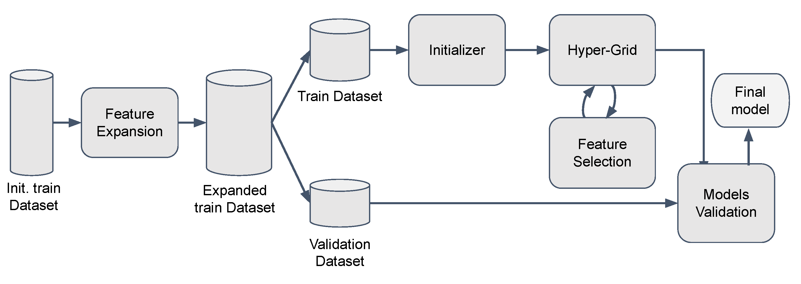
  • Design an auto-calibrated mosquito forecasting model:This combines Earth Observational and entomological information. Our approach allows for a generic framework that wraps itself around each case through automated feature selection and hyper parameters tuning process. This approach of feature selection prevents the injection of human bias into the model, while allowing for further analysis on the selected feature set. Framework’s description is presented in Section 3.
  • Accurate robust forecasting model, tested in actual measurements: This is for mosquito populations, independently of location and genus contextual constraints. The ML approach followed in combination with the automated selection of features enabled for an auto adjusted and accurate framework validated upon five different cases (consisting of 4 different areas of interest and 3 different mosquito species), with different contextual constraints delivering high performance presented in Section 4.
  • Comparative study: This is due to the replicability of our framework that uses the same architecture and the same mathematical principles offers the extensive capability of comparative studies among different cases, responding to: “which characteristics seem important in one case and which in another?” We can see in the comparative study of Section 4.
To the author’s knowledge, this is the first time that a single data-driven architecture has predicted mosquito populations of different species in a way that tackles several MBDs simultaneously and is independent to the site of application, thus presenting a high rate of transferability in different landscapes and climatic zones.
In the remaining parts, the paper is organized as follows: Section 2 presents the collection, augmentation and prepossessing of the entomological and EO data. In Section 3, a detailed description of the entire architecture with all the corresponding self-learning modules is given. Section 4 presents the case studies in which the system was applied, and the corresponding performance is reported and analyzed. Section 5 is a discussion of the results and the next research steps.

2. Datasets

This section presents the components of the preparation of the dataset and includes the collection of the Earth Observation and the entomological data, as well as their preparation to be used from the ML algorithms.

2.1. Open EO Data

The predictive model uses environmental variables (geographical, climatic, and hydrological) that influence the transmission cycle between pathogens, vectors, and hosts.
This study used remote sensing indices that have shown strong correlation with mosquito behavior and biological cycle. To compute the satellite derived Normalized Indices, a number of the satellite’s band were used, namely the Near Infrared (NIR), the Red (RED), the Short Wave Infrared (SWIR), and the Green (GREEN) band, as shown in formulas (1)–(4). The Normalized Difference Vegetation Index (1) (NDVI), the Normalized Difference Water Index (2) (NDWI), the Normalized Difference Moisture index (3) (NDMI), and the Normalized Difference Build-up Index (4) (NDBI) are used as proxies for vegetation density, changes in vegetation water content, determination of vegetation water content, and mapping of built-up areas, respectively. To quantify these environmental indicators for the period from 2010 to 2020, the satellite images Sentinel 2 (10 m GSD, 6-days revisit time) and Landsat TM 7 & 8 (30 m GSD 16-day repeat cycle) were accessed and pre-processed. The images were resampled to a uniform grid of 500 m × 500 m to obtain a spatially harmonized dataset.
N D V I = ( N I R R E D ) ( N I R + R E D ) ,
N D W I = ( G R E E N N I R ) ( G R E E N + N I R ) ,
N D M I = ( N I R S W I R ) ( N I R + S W I R ) ,
N D B I = ( S W I R N I R ) ( S W I R + N I R ) .
Temperature affects several processes associated with the mosquito, as well as the rate of virus development within the vector is associated with warmer temperatures [24]. The MODIS sensor from TERRA & AQUA was used to estimate Land Surface Temperature (LST), which is estimated from top-of-atmosphere brightness temperatures from the infrared bands of the satellite’s sensors. The product incorporated into the model is the V6.0, which provides daily LST daytime and nighttime values and emissivity with a spatial resolution of 1 kilometer (km).
Precipitation can have both a positive effect on the larval carrying capacity of breeding sites and a negative effect on the mosquito reproductive cycle interrupting it by flushing away aquatic stages from container breeding sites [25]. The Integrated Multi-satellitE Retrievals for GPM (IMERG) precipitation grid with a resolution of 0.1 × 0.1 was used to extract the daily precipitation on the day each trap was placed. The accumulated rainfall values for one week, and two weeks before each trap’s date of placement, as well as accumulated rainfall from the 1st of January of each year, were also calculated.

2.2. Meteorological Data

High wind speed is correlated with lower abundances of infected mosquitoes in traps. It seems that, in high wind speed situations, the reduced flying and biting activity of mosquitoes lead to lower transmission rates of WNV [26]. The ERA-5 Land Search Results Numerical Weather Prediction product was used with a native spatial resolution of 0.1 × 0.1 (hourly u and v components at 10 m). Further processing resulted in retrieving the hourly wind components from the relevant GRIB ERA5-Land file at the point-date level and calculating the daily min, max, and mean values including the dominant wind direction.

2.3. Auxiliary Data

Topography has been indicated as a significant factor in the transmission of MBDs, while it also influences the biotic conditions of different mosquito species and indicates the most suitable breeding sites. The Digital Elevation Model (DEM) product used to generate parameters, such as elevation, slope, and aspect, was acquired from Copernicus LMS with a spatial resolution of 25 m. For each point (trap station, WNV reported human case, village), the mean elevation, slope, and aspect were calculated within a buffer zone of 1 km around the point. The buffer radius was determined based on the flight range of the Culex spp. [27].
The challenge of processing big time series satellite data from different sensors at EU level and generating the relevant indices for the last 10 years was addressed by using the cloud-based geospatial processing platforms CREODIAS and Google Earth Engine (GEE). CREODIAS has been adapted to process big EO data, including a EO data storage cluster that allows live access to the entire Sentinel data collection at any time, without the need to submit a job to Cloud Archive and wait for it to become available. In turn, GEE is another big EO data analysis platform that has been used complementarily for the collection and processing of Landsat TM 7 & 8 and MOD11A1 V6 imagery by taking full advantage of the open source API Earth Engine Python and Earth Engine Catalog, enabling for fast computations.

2.4. Remote Sensing Data Preparation

The multi-spectral satellite data obtained from various sensors with different spatial and temporal resolutions had to undergo spatial and temporal integration. The higher resolution satellite sensors have been pre-processed and spatially resampled to 500 m by aggregating the information of the native pixel resolution of 30 m GSD in case of Landsat TM 7 & 8 and 10 m GSD in case of Sentinel 2. The MODIS the native spatial resolution of 1 km was resampled to 500 m by splitting the pixel into 4 equal value pixels. To deal with the diverse revisit time of the satellites, the data have been temporally resampled following the every other week circle of the entomological collection, by choosing the last available record. Since the EO data used were optical, we had to set a time threshold for the last available record for missing values due to cloud coverage. Therefore, the time window to search for the last available value has been set to one week for the LST and to one month for the indices. If no data were found during this time window, the value was assigned as missing value. For each of the in total 19,000 in-situ observations that were distributed in 4 countries, 21 EO variables were computed (see Table A1 in Appendix A for a detailed description of features). The term observation refers to one in-situ trap observation within a single time stamp. The EO variables were retrieved by processing big data with the volume of the satellite imagery approaching 200 Tb.

2.5. Entomological Network

A systematic approach for entomological monitoring has been effective since 2010 for Europe, collecting data from stable station networks. The entomological surveillance of the AOI in this work has made use of CDC-CO2 light traps and gravid traps, collecting mosquitoes each year on roughly every other week basis, identifying the total number of mosquitoes and the number of mosquitoes tested positive to the pathogen. As an example, Figure 1 depicts the entomological network in the Veneto region of Italy.

2.6. Data Pre-Processing

Final datasets, formed after the integration of multi source data, suffered from inconsistencies/erroneous insertions that had to be tackled. Duplicates of records were removed, while missing values in the dataset were filled using the method of iterative imputation, by modeling each feature with missing values as a function of other features in a round-robin fashion [28].
The range of several features varies a lot, which may be a problem when used with ML algorithms. The variance of the features with greater magnitude might contribute that much on the cost function and vanish the features with smaller magnitude. So, a normalization from −1 to 1 was applied to the indexers, to ensure that all indexers will be treated equally from the learner.

3. MAMOTH Principles and Methodology

In the usual supervised ML setting, we assume an initial dataset X consisting of a number of observations (rows) and a number of features (columns) called the feature-space. Additionally, each observation corresponds to a label/target variable y that should be estimated y ^ from the ML model f ( · ) by observing the input information X and a set of learnable parameters ϑ ,
f ( X | ϑ ) = y ^ .
In our case, X is the set of EO and entomological features that we know, θ are the internal parameters of the model, and y ^ is the prediction about the mosquito abundance for the upcoming period. The goal of the ML algorithm is to find, through the training process, the optimal learnable parameters ϑ of the model that minimize the cost between the real target of each observation and the corresponding estimated one. The aforementioned approach raises three fundamental modeling questions that should be specified: (i) Cost function—What do we aim to solve? (ii) Feature space selection—Which representation of the input is suitable for the optimization process? (iii) Solver—How are we going to solve the optimization problem?
In this section, we present MAMOTH, a framework for Mosquitoes Abundance Prediction Model, by answering the above modeling questions. As mentioned (see introduction section), MAMOTH main characteristic is that the user does not have to specify the feature space of the observations or models hyper-parameters. Instead, an auto-calibrated model is created based on the proposed architecture described in Figure 2 that receives the initial dataset and self-tunes its hyper-parameters. It decides which features to use build a custom prediction model that is meaningful for the AOI each time.

3.1. MAMOTH’s Cost Function

We transform mosquitoes’ populations from a regression to an ordinal classification problem, that offers multiple advantages both in the technical domain and in disseminating the results to a non-technical audience. Technically, this transformation makes our model more robust to outliers since the contribution of a single observation’s error is limited. In terms of dissemination, it helps a non-technical audience to understand the results e.g., “In the next two weeks, the model expects a mosquito abundance class 8 out of 10 for this region”, is more informative compared to “In the next two weeks, the model predicts an average of 183 Culex mosquitoes for this region”.
Accordingly, the cost function aims to minimize the Mean Absolute Error (MAE) between the real and predicted mosquito abundance classes.
M A E = 1 n i = 1 n y i y ^ i .
It is worth mentioning that the results obtained with MAE criterion (and being presented in Section 4) are similar to the results obtained with the mean square error criterion for the cases studied so far. Due to the analytical properties of the mean square error criterion, the training of the model is computationally much lighter than with mean absolute error criterion, so it can be used when we need a fast re-training of the models.

3.2. MAMOTH’s Feature Space and Solver

From the initial feature space, as described in Section 2, MAMOTH automatically decides on the proper number of features and the features themselves for every specific case (different mosquito species or different area). The solver of the model is relying on Gradient Boosting ML technique for regression. Gradient Boosting machines belong to a very powerful and popular family of ensemble techniques that combine numerous weak learners in order to produce a powerful learner [29]. The parameters that have to be tuned are the max depth of the trees constructed and the number of estimators (number of trees) since our gradient boosting model relies on decision trees. In regard to the purpose of the parameters, the tree depth indicates the complexity capabilities of the algorithm, and the number of estimators refers to the quantity of estimators that will be used with the sequent estimator correcting the previous one. The hyper-parameters of the solver, as well as the selection of the feature space, are automatically specified by MAMOTH, as illustrated in the pipeline of Figure 2.
Description of MAMOTH’s pipeline: As depicted in Figure 2, the model’s architecture consisted of 5 main modules: (i) Feature Expansion/Engineering, (ii) Pre-process, (iii) Parameters Grid, (iv) Feature Selection, and (v) Model Selection. The main advantage of this architecture is that, even if the final model is complex, each module, separately, is simple, and its functionality is quite intuitive. This advantage is crucial for the implementation and the further evolution of the model.

3.3. Feature Extraction/Engineering Module

The information that is already included in the dataset can be used/restructured to generate new features that are informative regarding the target variable in a more algorithm-friendly way. This process requires a strong understanding of the physical problem and a good knowledge of the related work to guide the selection of valuable features for the ML algorithms. This process involves various operations on the feature space, such as (i) non-linear transformations, (ii) linear and non-linear combinations, (iii) temporal and spatial shifts, (iv) moving averages, (v) variables related to spatial clustering of the data, (vi) strong components of PCA, and (vii) thresholds for variables. The goal is to provide a more extended pool of features to the next modules. Respecting the trade-off between information and complexity leads us to the most limited number of features that capture spatial and temporal information that could be useful for prediction. At this point, it should be stated that removing this module out of the framework’s pipeline is possible, but, based on our experiments, this led to an average 20% decrease in the performance. The features used in this paper can be found in the Appendix A in Table A1.

3.4. Initialization Module

This module obtains as input the training set and starts the initialization of the training process (i) Determine the mosquito abundance classes: Calculate the range of each abundance class and perform balance handling if needed. The range of each class is selected so that all classes have equal probability of selection. In this paper, the number of mosquito abundance classes is set to 10 (ii) Target set: the optimal time distance for prediction according to the training set is selected or proposed to the user, e.g., predict the mosquito abundance for the next 15 days or 30 days. To determine the optimal time distance for the target set, a CDF (Cumulative Distribution Function) of the time distance of days between two consecutive observations was created, and the minimum time distance that covers as much of the dataset as possible is selected. (iii) Initial tuning: uses the most correlated features (according to Pearson correlation score) to make an initial rough estimate on the hyper-parameters of the model in a gradient-based manner (max_depth, number of estimators).

3.5. Hyper-Parameters Grid Module

It takes as input the initial estimate of the model’s hyper-parameters and generates parameters’ grid points around these values. For each of these points, the Feature Selection module outputs a single model. This stage is useful for further fine-tuning the model’s hyper-parameters. This module improves the overall performance of the model, but we should mention that, in most of our experiments, this improvement was less than 7%. So, in case of limited computational resources, we can skip this module and build a mode directly in the initial estimation of the hyper-parameters of Initialization Module.

3.6. Features Selection

For each point in the parameters’ grid, the system starts with the entire set of features, as specified in the feature extraction/engineering module, and uses recursive feature elimination and cross-validated selection to select both the optimal number of features in the feature space and the features themselves. In the feature elimination, the ranking of each feature is done according to the usual relative importance score [30]. Finally, we use the coefficient of determination, known as R2 score, in a 10-fold cross-validation set to select the model with the optimal number of features. This process slightly increases the complexity of the model (k-fold cross-validation is a linear operation in terms of resources) but makes the model more robust to randomness and bias.

3.7. Model Selection

Finally, each model of the grid point is evaluated with unseen validation data, and the final model is selected according to the mean absolute error criterion (optionally, this criterion can be changed to the mean squared error).
The model’s predictions are assessed using the same metric as the cost function used during the training phase, the MAE. This metric indicates the distance between the actual class and the predicted class, which gives a simple intuition of the quality of the prediction. Another metric that can characterize the quality of the system is the percentage of predictions with an error equal to or less than 3 classes. This metric quantifies the percentage of the time that the predictions do not deviate too much.

3.8. Computational Cost

A fundamental aspect of a machine learning model is the computational cost (complexity). Our framework uses a Gradient Boosting model as learner, so, it is directly affected by decision tree cost, which is equal to O ( m n d ) [31], where n is the number of observations in the training set, m is the number of features, and d is the depth of the tree. Since Gradient Boosting Models construct M different decision trees, the model’s computational cost is O ( M ( m n d ) ) . The framework applies a greedy search for optimal features by training multiple gradient boosting models and recursively eliminating the least significant feature; this increases linearly the overall complexity with respect to the number of features to O ( M ( m 2 n d ) ) . So, the more the features available, the more gradient boosting models will be constructed, and, thus, the higher the overall computational cost will be. Hyper-parameters grid module can also add in computational cost due to the repetition of the aforementioned process, as it executes exhaustive search in a window (e.g., of 5 × 5 ) around the initial hyper-parameters estimation (max_depth, number of estimators); this module multiplies the overall computational cost by a factor equal with the number of grid points (e.g., 25). It can be concluded that MAMOTH’s computational cost is affected quadratic by the number of features m used and linearly by the hyper-parameters tuning grid.

4. Experimentation

In the Experimentation section, we present the application of our framework to a total 5 different cases (three different mosquito species and four different areas). The cases cover scenarios that allow us to perform comparative analysis, such as the same mosquito species (Culex pipiens) in three different areas or two different mosquitoes species in the same area of interest.
We applied MAMOTH to the Veneto region in Italy to predict the population of Culex pipiens. These predictions took place on the trap site, since the model uses the historical entomological data as input features in the training process. The models’ performance was also tested for off-trap-site predictions with promising results; in this experiment, the training of the model did not use past entomological information as input features.
The validation of the framework was conducted in 2 different ways, operationally on last year’s data and pre-operationally. Operational validation is designed to imitate the real life conditions and pre-operationally validation operates on multiple random realizations (via k-fold validation) to verify that the received performance is not an outlier. More specifically, on the Operational validation, we test separately each month of 2020. When testing on a specific month’s data, the rest of the data past this month will be completely ignored by the training process as they belong to the future, and we know nothing about them. This process goes on iteratively to cover all available months of last year’s data. For example, if we want to predict the abundance of mosquitoes in July of 2020, observations until July of 2020 will be used as training set, while observations past July will be completely ignored. This method was applied iteratively in a cross-validation fashion to assess the model’s performance. Pre-operational validation is a classical 10-Fold cross-validation method where all observations are taken into account without any time constraints. This process rules out any performance inconsistency due to a specific time series behavior and verifies that the results of the operational validation is not an outlier. Results showed that the two kinds of validations perform similarly, with pre-operational validation achieving slightly better results as expected. In addition, we conducted experiments for a comparative study, and we applied the framework in Vojvodina (Serbia) and Baden Wuerttemberg (Germany) to further test its performance for the abundance of Culex mosquitoes. We also extended the model to two other species, Anopheles spp. in Veneto (Italy) and Aedes albopictus in Grand-Est and Corsica (France). In all these cases, the results were promising and consistent.

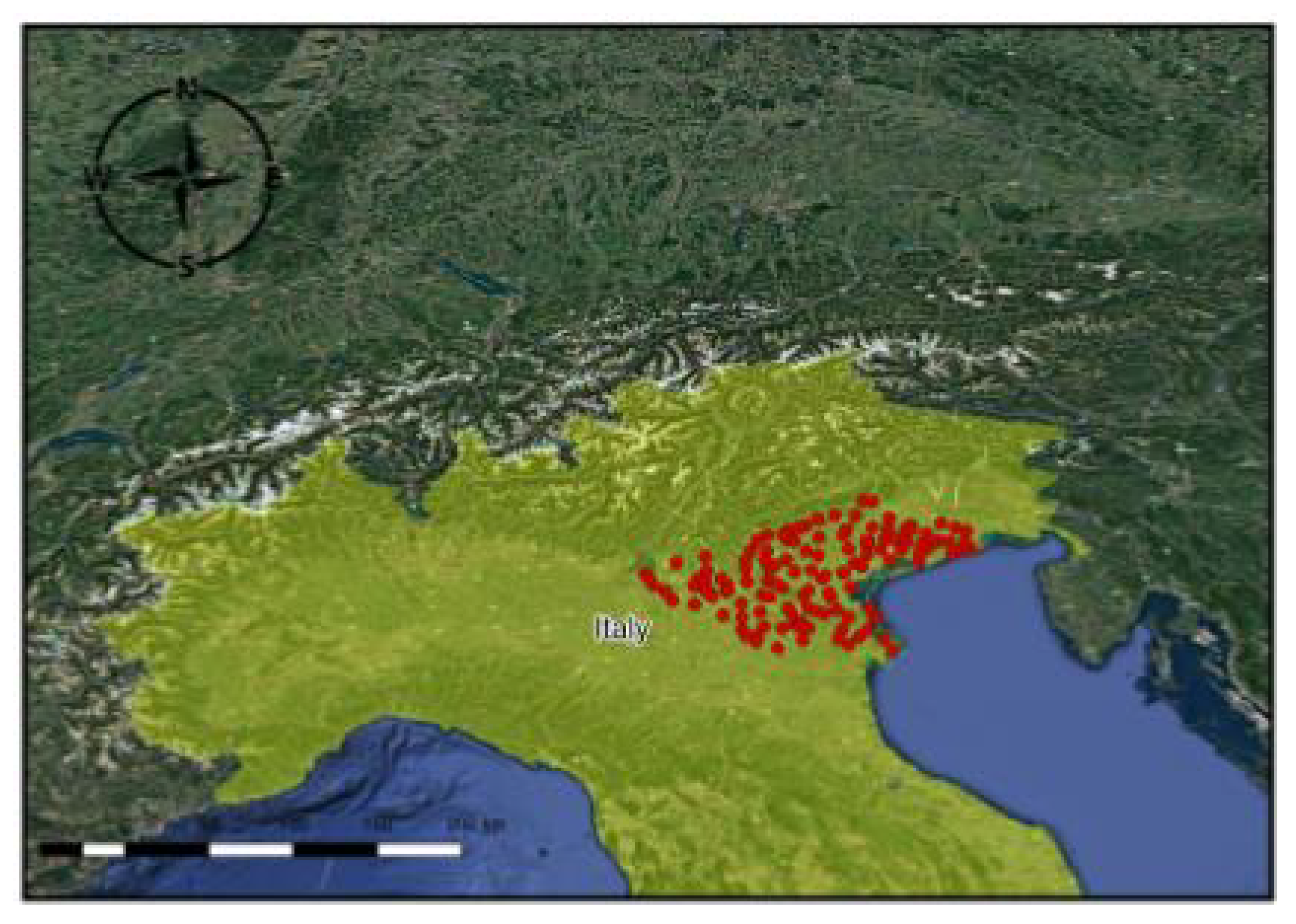
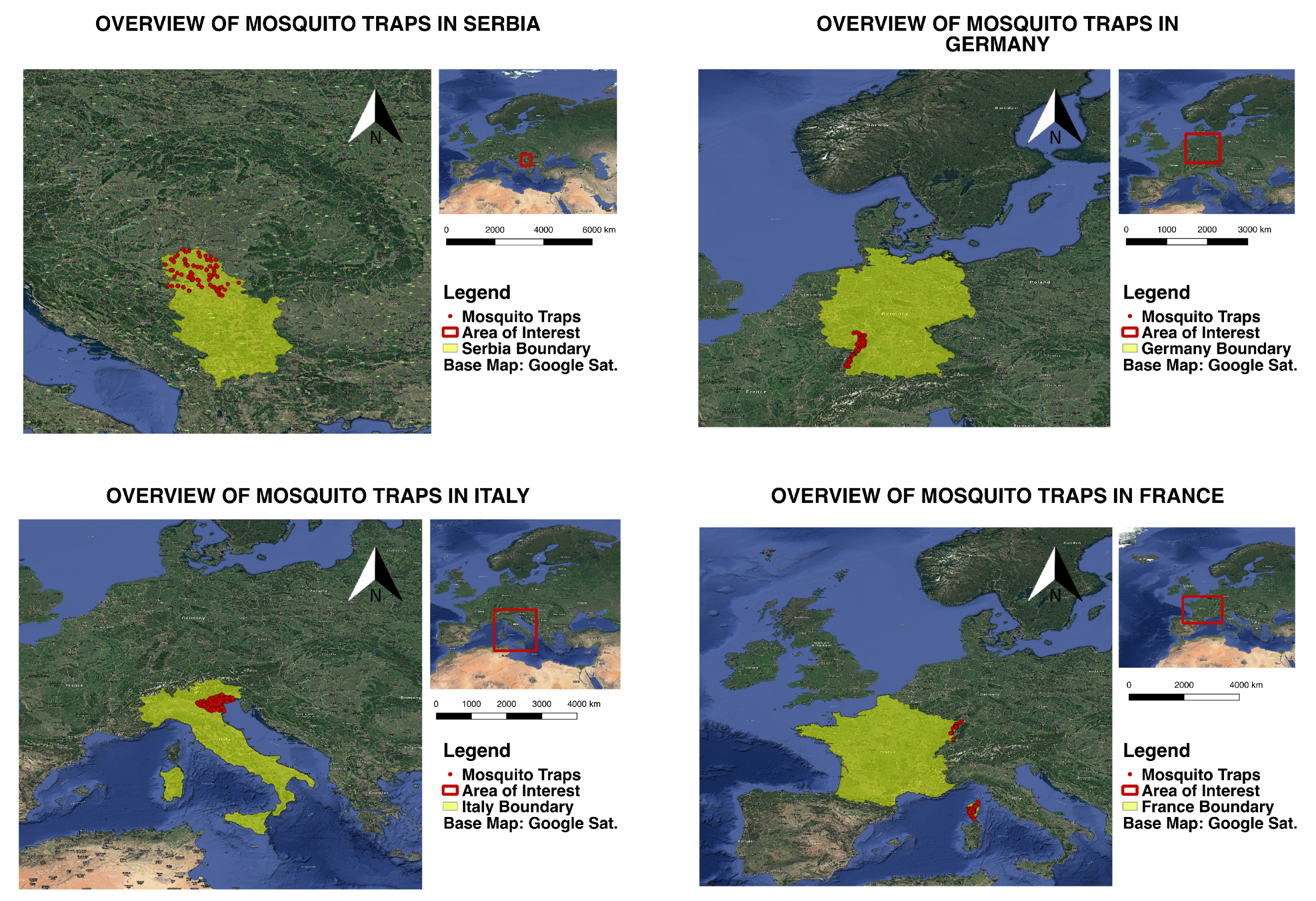
4.1. Area of Interest and Entomological Network

The study area is located in Northeast Italy, at the Veneto region, as depicted in Figure 1. The area includes the eastern part of the Alps and the northeastern part of the Po Valley. The average temperature during the period of interest had a mean value of 25.4 degrees Celsius, and the cumulative precipitation was 30 mm.
The entomological monitoring of Culex pipiens in the Veneto region has been effective from 2010 to 2020, gathering data from a network of 140 stations and resulting in a dataset of more than 4800 observations.
Table 1 presents class separation of the initialization module, and the corresponding number of mosquitoes for each class, as well as the probability of having at least one mosquito positive to WNV. It can be observed by Table 1 that the probability is monotonically increasing as the number of mosquitoes increases, which supports the claim that the higher the mosquito population the higher the WNV circulation and, thus, its dissemination in the community.
In case of Culex mosquitoes in Italy, nearly 80% of the observations had at most a 15 days time distance between two consecutive observations of the same stations, as shown in Figure 3. So, the target of prediction was set to 15 days to keep as many observations as possible while keeping a reasonable prediction time in order to grant authorities time to take preventive actions against mosquitoes if needed.
Furthermore, the auto-calibration process was tuned to max_depth = 5, number of estimators = 23, and and it was decided that the optimal number of features is 16. The selected features with their corresponding importance are presented in Figure 4.
It is clear that the most important feature which affects mainly the prediction of mosquito abundance class is the current mosquito population. Additionally, the accumulated mosquito populations of the running month seems to play an important role in the formation of the final prediction. Those two features are capturing the temporality in an indirect way, the current state is very important for the upcoming state, and seems to be important in all Culex mosquito cases independent of the area of interest. Temporality is directly captured by the days distance from a certain date regardless of the year, indicating that the mosquito population is partly following a pattern. Besides the temporality and mosquito population, though, presence of water is also a considerable factor as measurements on its different states are selected by the system by 3 different features (NDWI, two past weeks cumulative rainfall and cumulative from January rainfall). Temperature is also selected and represented by 2 features, however affecting much lower in the final prediction than expected based on relevant literature which claims that temperature is one of the main contributor for the mosquito population. Spatiality expressed by the latitude and elevation of the trap site are also features that the system chose to make more accurate predictions.

4.2. Culex Veneto Results

The MAE for all the predictions is 1.27. The error distribution in Figure 5 shows that most of the errors are spread across a small range, meaning that 97% of the predictions are less or equal to 3 classes away from the actual class. Those promising results show that the system’s predictions are, most of the time, very close to the actual mosquito population that we aim to predict.

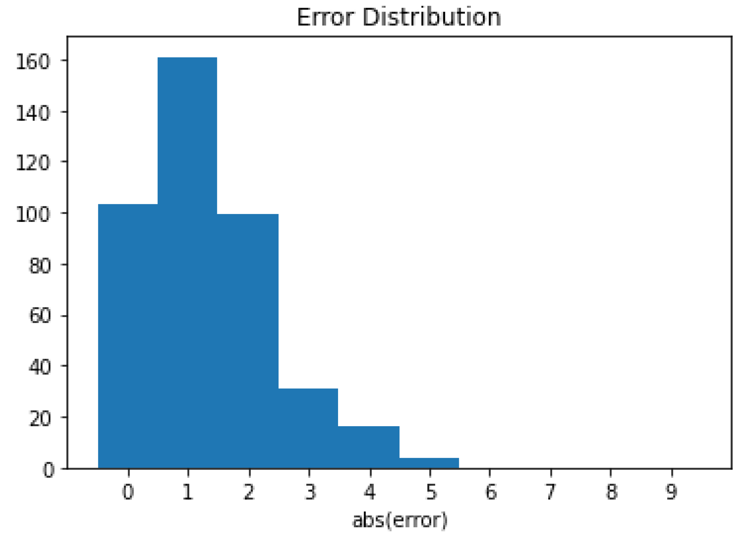
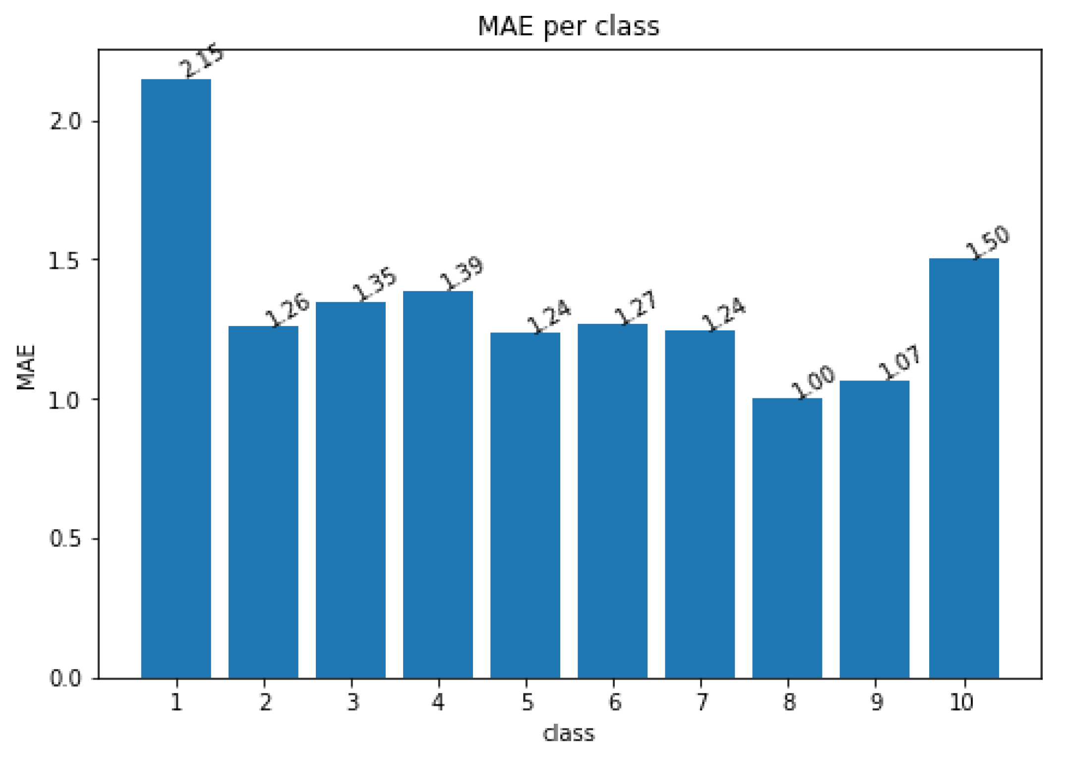
4.2.1. Error Distribution among Risk Classes

In the plot of error of each class in Figure 6, we can see that the model is performing similarly in all mosquito abundance classes, without any strong bias to low or to high abundance classes.

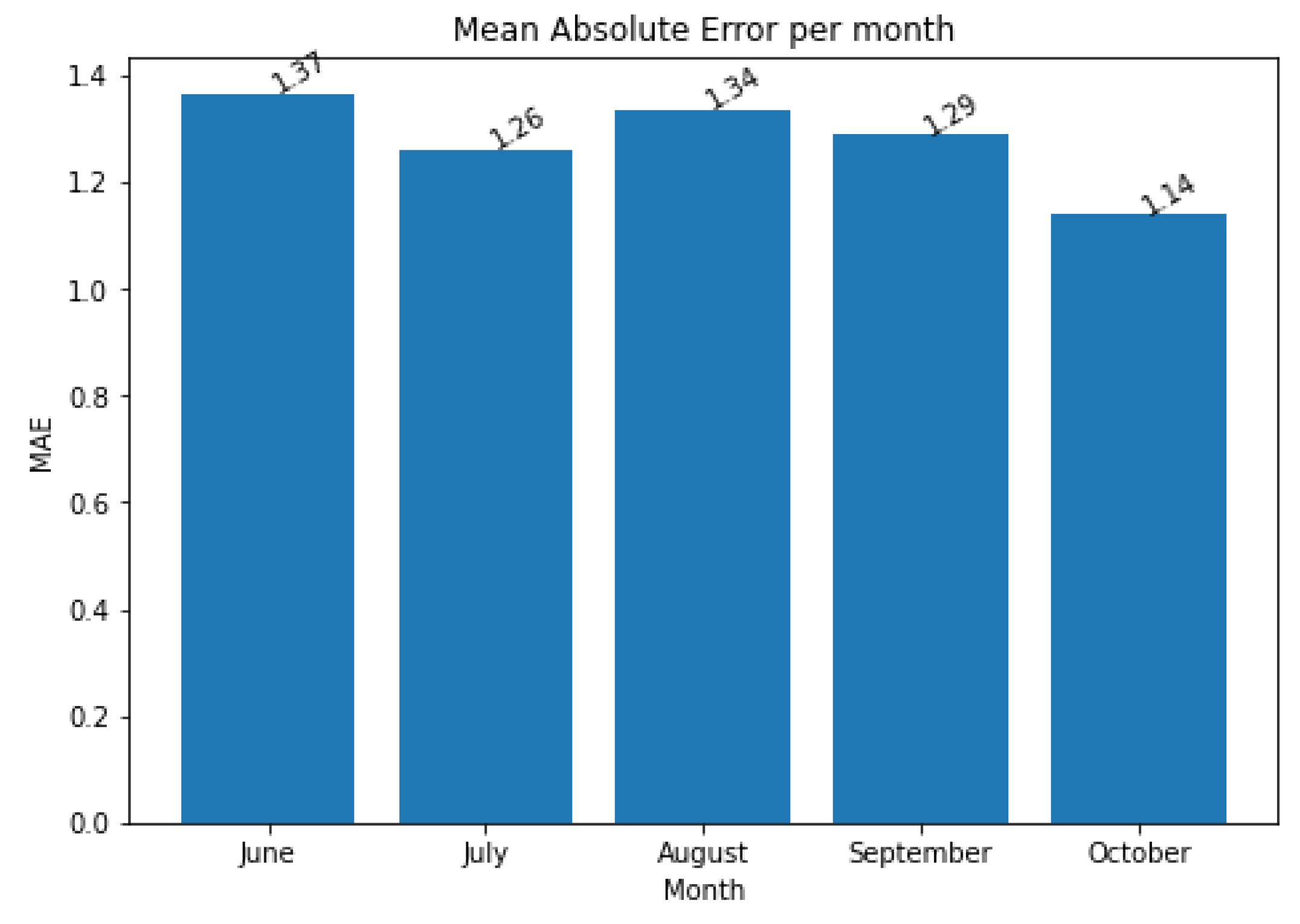
4.2.2. Results per Month

The prediction error of each month is relatively equal, the MAE in June is higher due to smaller size of dataset and the lack of data, before May of 2020, thus training the model only upon data of previous years and not in recent observations. Respectively, the MAE of October is lower than the others, due to the training of the model in many more recent observations, as shown in Figure 7.
To validate the performance of the model except the operational application, the system was tested on random 10-fold validation using all the available data. The results showed slightly better behavior, in terms of MAE: 1.14, and similar performance in terms of percentage of error below 3 classes: 97%. This slight improvement can be explained by the fact that, in the k-fold validation, the samples for train and test process are selected uniformly from the entire dataset compared to the operational case where train and the test sets are totally separated in time. Those results are leading us to the conclusion that the performance of the model is stable according to train-test separation of the dataset.

4.2.3. Performance without the Entomological Features

As depicted in Figure 4, the model relies a lot on the entomological features in order to predict the mosquito population for the upcoming period. The current number of Culex mosquitoes is the most important feature by far, while the feature with the third highest relative importance score also being the sum of Culex mosquitoes of the past 30 days, and the fifth highest feature on the list is the mosquito population of the same month the previous year. The need of those entomological features could limit the wide use of the model, once this information is known only on the trap-site. Away from the trap-sites, this information will not been known. Thus, the question that we like to answer is, could the model perform reliably if those important entomological features are missing from the feature space?
To test this hypothesis, we removed all features relevant to entomological data, and we re-trained a new MAMOTH model using only EO data and features derived from them. The results showed that the model was still able to accurately predict the upcoming mosquito population with a small accuracy reduction compared to the model that used entomological features. The new MAMOTH model performed with 1.65 MAE, and the percentage of errors below 3 classes was reduced to 92%. The wide applicability of a model that relies only on EO data marks those results as promising for further research in that direction.
As seen in Figure 8, the new model in order to fill the gap that was created by the absence of the entomological features, increased the total amount of selected features to 34 (compared to 16 of the model with the entomological features), along with the significantly increased importance of EO-related features, such as rainfall, LST, NDWI, NDVI, and NDBI.

4.2.4. Performance without the EO Features

As mentioned above, even in lack of entomological data, MAMOTH was still able to predict the upcoming mosquito abundance using only EO data and features derived by them. However, for the sake of completeness, it is of great importance to investigate the performance of the framework without using any EO data. To test the performance of the framework without the presence of EO data, we removed all the related EO features. The results showed that the performance of the model was a slightly decreased compared to the previous case where EO and entomological data were available. More specifically, the error climbed up to 1.34, and the percentage of errors below 3 classes was reduced to 94%, using 15 features.
As we can see in Figure 9, the model basically relies on the current mosquito population and the seasonality of the observation in order to deliver accurate predictions. This version of the model points out the significance of the entomological data, as without any EO information available the performance of the model was not deviating much from the initial model with EO and entomological information available. However, even in lack of them, a similar result can be achieved using only EO data.

4.3. Other Cases

MAMOTH was trained and validated with respect to its generic character and robustness in different cases of mosquito species and engaged regions (landscapes). Specifically, the model was implemented and returned high performance in (a) Serbia for the Culex pipiens (WNV), (b) Germany for the Culex pipiens (WNV), (c) Italy for the Anopheles spp. (Malaria), and (d) France for the Aedes albopictus (Zika, Chikungunya, Dengue).
Figure 10 depicts the areas of interest, and Table 2 presents the main characteristics of each data collection.
Table 3 presents cumulatively the performance of MAMOTH to the aforementioned cases. The results clearly reveal that, indeed, the MAMOTH framework is generic and easily replicable to other cases. It is also shown that, although the auto-tuned parameters are varying in the different use cases, the performance of the models remains stable and high, with the maximum accuracy being returned in the case of Aedes Albopictus in France, where the MAE is surprisingly low.
Table A2 also presents the performance of MAMOTH to the aforementioned cases, but this time using only environmental data, proving the claims that the proposed framework is also applicable to regions without any previous knowledge of the current entomological situation, while Table A3 presents the performance of MAMOTH without any EO data available. Both of these tables can be found in the appendix Section.
The 13 most important features, selected by MAMOTH, and their corresponding importance for each case of interest are presented in the Table 4. In addition, Table 5 presents the 5 five most significant features per PCA component, so as to provide all the information needed for drawing accurate conclusions. By comparison between the different cases, we can draw some insights:
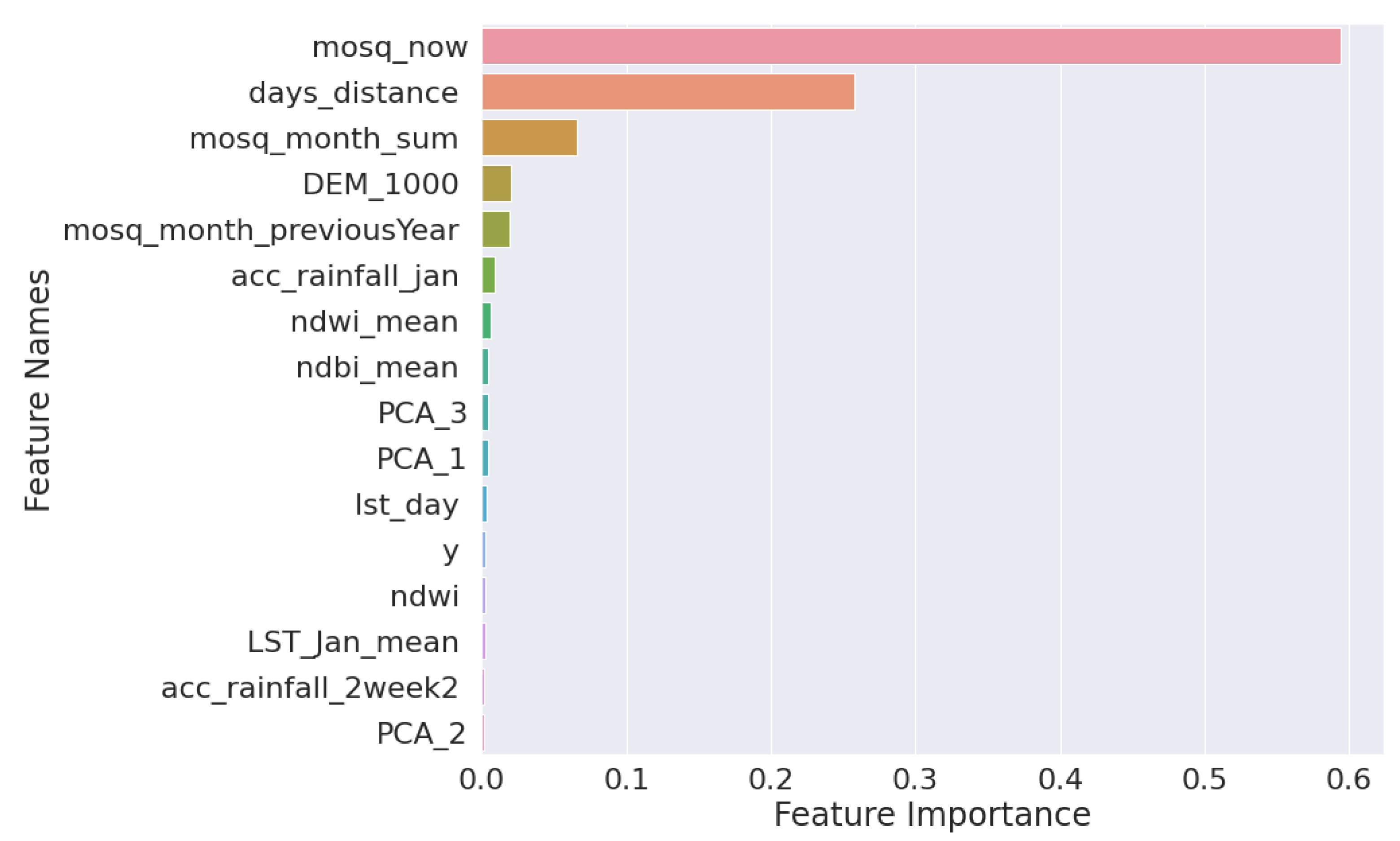
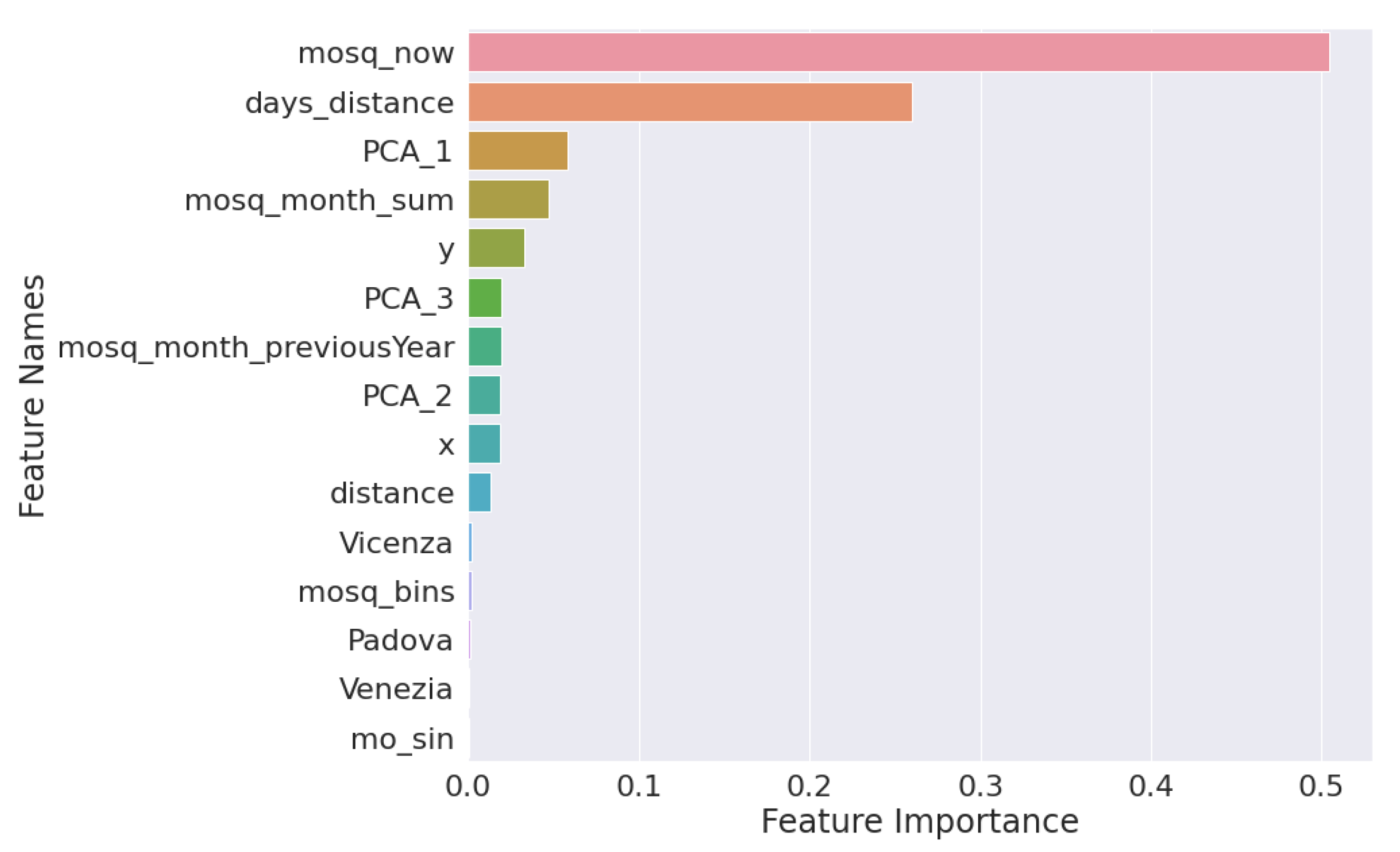
  • For all cases, previous mosquito populations seem to play a preponderant role, as is expected for the seasonal development of mosquito populations during summer months, depending on the intensity of mosquito control applications in the AOI.
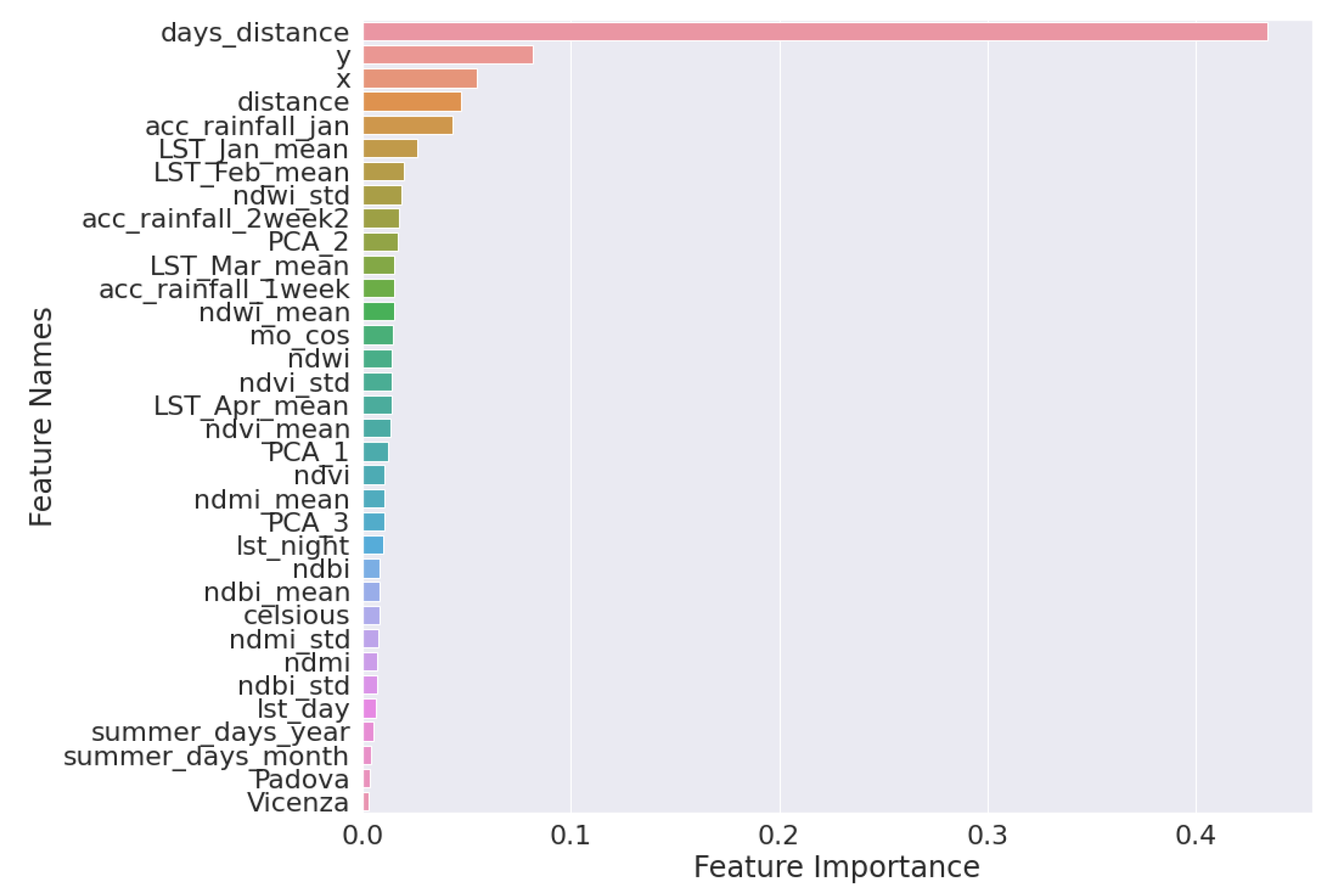
  • The accumulated rainfall from the beginning of the year is important for all the cases, and, for the cases of Culex spp., the accumulated rainfall of the last two weeks seems important, as well.
  • In all Culex spp. cases, the rainfall and the water indices, NDWI, are more important than the temperature, LST.
  • Anopheles is the only mosquito genus in which the most important feature is not the previous state of the mosquito population but the direct time distance, as well as several geomorphological features, which could indicate the preference of mosquitoes of this genus of stagnant water surfaces in specific altitudes.
  • Aedes albopictus prediction is the only case where the direct time distance is not important for the model. Furthermore, the Aedes albopictus populations seem to be very sensible to temperature, more than to precipitation, while both are important factors for the creation and durability of breeding sites for this container breeding species.
  • NDWI metrics are very important for the prediction of Aedes albopictus populations compared with the other mosquito species.
Table A4 and Table A5 that present the most significant feature per case using only EO data and without using any EO data, respectively, can be found in the appendix Section.

5. Discussion/Conclusions

In this paper, we saw that it is feasible to develop a generic machine learning model that predicts mosquito populations without any special design regarding the area of interest or the mosquito species. We prove that this approach achieves accurate and reliable performance, by relying on common satellite and entomological data. Additionally, this direction gives us the opportunity of comparative study between different areas or mosquitoes.
The results show that, indeed, the model manages to be auto-calibrated for the different cases by selecting different features and parameters. Additionally, our approach offered the capability of comparative studies and the extraction of valuable information, without which a generic and unified approach could not have been possible.
Furthermore, the results of MAMOTH for predictions away of the trap-site, if the model is trained only upon environmental and not past entomological data, were promising, as the performance did not deviate much from the initial model. Thus, even in lack of entomological data, the system remains robust and able to predict mosquito populations. This variation of the system offers a more flexible model, applicable even to communities that do not have dense entomological networks, once the model can extrapolate the mosquitoes abundance between the traps. However, the use of entomological data offers valuable information to the model, allowing for more accurate predictions. An important difference between the two models, however, is the number of features selected by the model. In the second case, where only EO data are used, the number of features is significantly larger. This direction of research is quite promising once the off-trap site prediction massively increases the applications of the model.

Author Contributions

Conceptualization, E.P., G.A., and C.K.; methodology, A.T., E.P., G.A., A.V. and C.K.; software, A.T. and E.P.; validation, A.T. and G.A.; formal analysis, A.T. and G.A.; investigation, A.T.; resources, A.V.and C.K.; data curation, A.T., K.K. and S.G.; writing—original draft preparation, A.T., E.P. and G.A.; writing—review and editing, A.T., E.P., G.A., K.K., S.G., A.V. and C.K.; visualization, A.T. and E.P.; supervision, G.A., A.V. and C.K.; project administration, K.K. and C.K.; funding acquisition, C.K. All authors have read and agreed to the published version of the manuscript.

Funding

This research was partially funded by framework service contract for Copernicus emergency management service risk and recovery mapping.

Acknowledgments

MAMOTH was developed in the framework of the EYWA project, an EarlY WArning System for Mosquito-Borne Diseases, an initiative under the flag of the EuroGEO Action Group “EO4EViDence—Earth Observation for Epidemics of Vector-Borne Diseases”. We would like to specially thank our partners for their entomological data contribution, namely the Istituto Zooprofilattico Sperimentale delle Venezie, and the Veneto and Friuli-Venezia Giulia Regions for Italy’s data; the Faculty of Agriculture in the University of Novi Sad for Serbia’s data; the Kommunale Aktionsgemeinschaft zur Bekämpfung der Schnakenplage e.V. for Germany’s data; and the Entente Interdépartementale pour la démoustication du littoral Méditerranéen for France’s data.

Conflicts of Interest

The authors declare no conflict of interest.

Appendix A

Table A1. Feature list.
FeatureExplanation
dt_placemeDate of the observation
stationidStation ID
xLongitude
yLatitude
mosq_nowMosquito population in trapping sites at the date of observation
NDVIProxy for the vegetation density and distribution
Extracted pixel value of overlapping station ID coordinates
NDVI_meanProxy for the vegetation density and distribution
Mean value of neighboring pixels (window of 3 × 3)
NDVI_stdProxy for the vegetation density and distribution
Standard deviation of neighboring pixels (window of 3 × 3)
NDWIProxy for changes in water content
Extracted pixel value of overlapping station ID coordinates
NDWI_meanProxy for changes in water content
Mean value of neighboring pixels (window of 3 × 3)
NDWI_stdProxy for changes in water content
Standard deviation of neighboring pixels (window of 3 × 3)
NDMIProxy for determination of vegetation water content
Extracted pixel value of overlapping station ID coordinates
NDMI_meanProxy for determination of vegetation water content
Mean value of neighboring pixels (window of 3 × 3)
NDMI_stdProxy for determination of vegetation water content
Standard deviation of neighboring pixels (window of 3 × 3)
NDBIProxy for mapping urban built-up areas
Extracted pixel value of overlapping station ID coordinates
NDBI_meanProxy for mapping urban built-up areas
Mean value of neighboring pixels (window of 3 × 3)
NDBI_stdProxy for mapping urban built-up areas
Standard deviation of neighboring pixels (window of 3 × 3)
LST_dayLand surface temperature at day
LST_nightLand surface temperature at night
LST_Jan_meanMean temperature in January
LST_Feb_meanMean temperature in February
LST_Mar_meanMean temperature in March
LST_Apr_meanMean temperature in April
wind_maxMax magnitude of wind
wind_meanMean magnitude of wind hourly
wind_minMin magnitude of wind
acc_rainfall_1weekAccumulated precipitation counting towards
one week before the date of placement
acc_rainfall_2week2Accumulated precipitation counting towards
two weeks before the date of placement
acc_rainfall_janAccumulated precipitation counting
from the 1st of January of each year
WC_L_1 kmCombination of breeding site length and water course of national
hydrological data within a buffer zone of 1000 m around each
sampling/trapping site
PG_area_1 kmTotal area of temporarily inundated areas (polygons)
within a buffer zone of 1 km from each sampling/trapping site
DEM_1000Mean elevation (resolution = 12.5 m),
within a buffer of 1000 m around trapping sites
Aspect_1000Mean aspect (12.5 m),
within a buffer of 1000 m around trapping sites
Slope_1000Mean slope (12.5 m),
within a buffer of 1000 m around trapping sites
Coast_dist_1000Mean Distance of sampling/trapping site
within a buffer of 1000 m from coastline
WC_dist_1000Distance of combination of breeding site length and length of
watercourses of national hydrological data within a buffer zone
of 1000 m around each sampling/trapping site
Flow_acc_1000Mean flow accumulation within a buffer of
1000 around trapping sites
mosq_month_sumCumulative mosquito population of the past 30 days
mosq_month_previousYearCumulative mosquito population of the month on previous year
mosq_binsMosquito bin based on the population on the date of observation
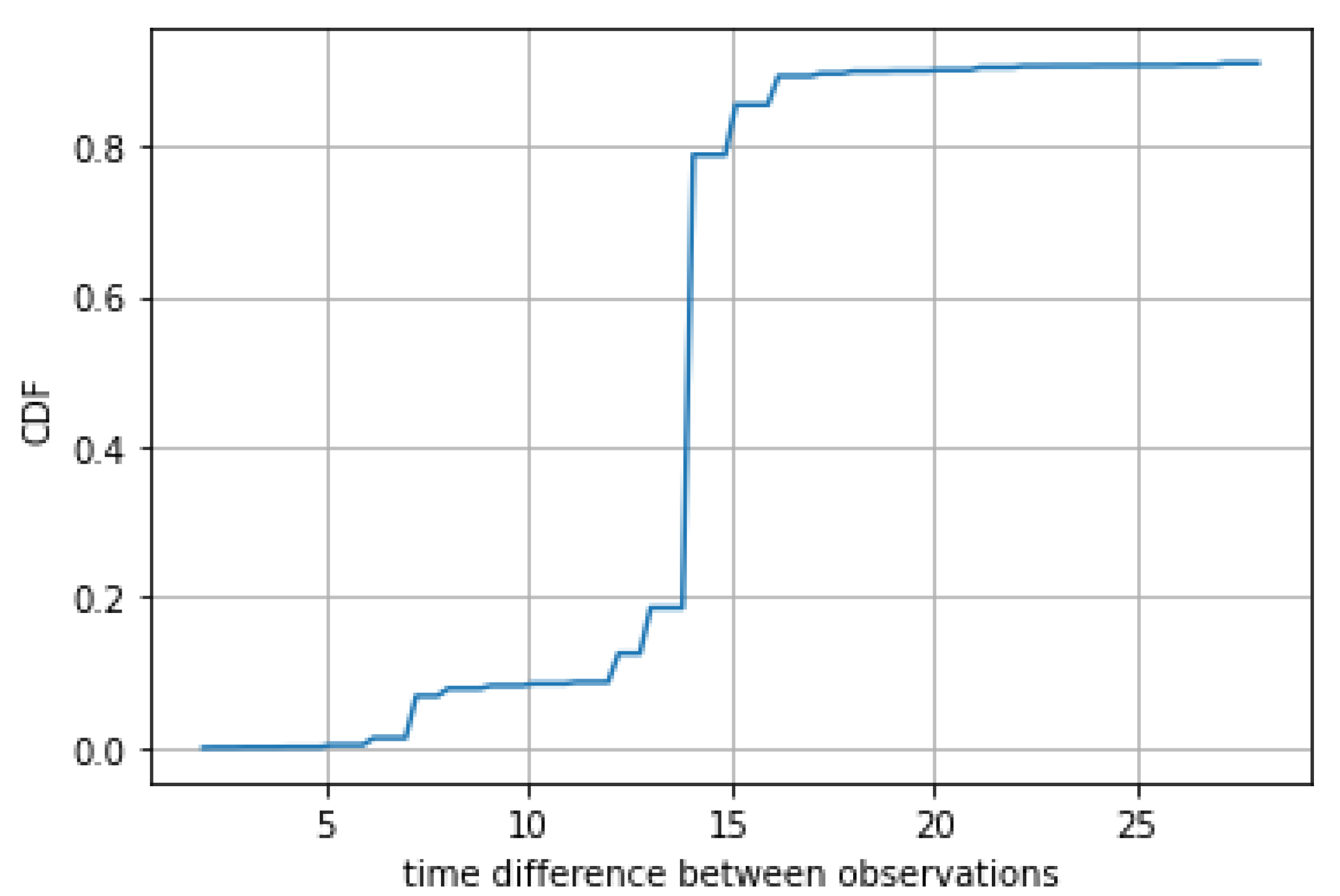
days_distanceTime difference in days between the date of
placement and a specific date regardless the year
province (multiple features)Province in which trap is located (transformed in one hot encoded
features out of the names of the provinces of each region)
mo_cosCosine transformation of the month of date of placement
mo_sinSine transformation of the month of date of placement
celsiusLST_day to celsius conversion
summer_days_yearDays with over 30o celsius within the year
summer_days_monthDays with over 30o celsius within the month
PCA components3 PCA components extracted from the whole dataset
distanceEuclidean distance of coordinates between
a specific point and the trap site
Table A2. MAMOTH’s pre-operational applications and performance per country using only EO data.
Area of Interest
Mosquito
Auto-Tuned
Model Parameters
MAE in
Nb Classes
Prediction < 3
Classes Error
Serbia Culex spp.Nb of features = 37
Nb_estimators = 11
Max_depth = 14
test = 1.88, train = 0.8187%
Germany Culex spp.Nb of features = 22
Nb_estimators = 31
Max_depth = 4
test = 1.18, train =1.0789%
Italy Anopheles spp.Nb of features = 51
Nb_estimators = 33
Max_depth = 6
test = 1.48, train = 0.5494%
France Aedes albopictusNb of features = 42
Nb_estimators = 20
Max_depth = 14
test = 0.72, train = 0.9687%
Italy Culex spp.Nb of features = 34
Nb_estimators = 27
Max_depth = 9
test = 1.20, train = 0.6096%
Table A3. MAMOTH’s pre-operational applications and performance per country without using any EO features.
Area of Interest
Mosquito
Auto-Tuned
Model Parameters
MAE in
Nb Classes
Prediction < 3
Classes Error
Serbia Culex spp.Nb of features = 3
Nb_estimators = 20
Max_depth = 7
test = 1.73, train = 1.1886%
Germany Culex spp.Nb of features = 4
Nb_estimators = 28
Max_depth = 4
test = 1.04, train = 0.9990%
Italy Anopheles spp.Nb of features = 20
Nb_estimators = 26
Max_depth = 9
test = 1.54 train = 0.2792%
France Aedes albopictusNb of features = 13
Nb_estimators = 26
Max_depth = 3
test = 0.74, train = 0.6391%
Italy Culex spp.Nb of features = 15
Nb_estimators = 24
Max_depth = 8
test = 1.16, train = 0.7695%
Table A4. Most important features per case without using EO data.
Aedes-FranceAnopheles-Italy
feature namesimportancefeature namesimportance
mosq_now0.561days_distance0.303
days_disance0.200mosq_now0.209
PCA_30.049distance0.077
mosq_monh_sum0.040mosq_monh_sum0.077
PCA_10.035mosq_monh_previousYear0.072
PCA_20.031PCA_30.071
x0.026PCA_10.067
y0.022PCA_20.063
mo_sin0.017Treviso0.012
mosq_month_previousYear0.015Padova0.010
distance0.004Rovigo0.009
HAUE-CORSE0.000mosq_bins0.009
mosq_bins0.000Venezia0.008
Vicenza0.004
mo_sin0.002
Verona0.002
Gorizia0.002
mo_cos0.002
Pordenone0.001
Udine0.000
Culex-SerbiaCulex-Germany
feature namesimportancefeature namesimportance
PCA_10.397mosq_now0.592
days_distance0.388mosq_bins0.223
mosq_monh_previousYear0.215mo_cos0.105
PCA_30.079
Table A5. Most important features per case using only EO data.
Aedes-FranceAnopheles-Italy
feature_namesimportancefeature_namesimportance
x0.150days_distance0.274
lst_night0.137DEM_10000.082
PCA_20.059PCA_30.049
ndwi0.055ndwi0.041
ndvi0.039Slope_10000.039
acc_rainfall_2week20.038LST_Jan_mean0.038
ndvi_std0.038PCA_20.038
days_distance0.035ndwi_std0.033
ndwi_mean0.034ndvi_std0.032
PCA_10.033ndvi_mean0.026
ndmi0.031lst_night0.023
ndbi_mean0.030acc_rainfall_jan0.023
PCA_30.028ndwi_mean0.023
acc_rainfall_jan0.026celsius0.021
ndvi_mean0.024lst_day0.021
summer_days_month0.024acc_rainfall_2week20.019
ndwi_std0.022acc_rainfall_1week0.016
acc_rainfall_1week0.021y0.015
ndmi_mean0.021ndmi0.014
distance0.020ndvi0.014
Culex-SerbiaCulex-Germany
feature_namesimportancefeature_namesimportance
days_distance0.118acc_rainfall_jan0.343
acc_rainfall_1week0.076days_distance0.158
mean_wind0.071y0.155
acc_rainfall_jan0.063distance0.058
PCA_30.037acc_rainfall_2week20.054
y0.035mo_cos0.025
PCA_20.034x0.023
DEM_10000.034ndmi_mean0.023
lst_night0.029WAW0.020
PCA_10.027lst_night0.017
Aspect_10000.027acc_rainfall_1week0.015
ndwi_std0.027ndvi_std0.014
max_wind0.025ndmi0.013
ndvi_mean0.024DEM_10000.011
LST_Jan_mean0.023LST_Apr_mean0.011
acc_rainfall_2week20.022LST_Jan_mean0.011
Slope_10000.020PCA_30.011
ndwi0.020ndwi0.009
Sremski0.018ndwi_mean0.009
LST_Feb_mean0.018celsius0.007

References

  1. World Health Organization. Vector-Borne Diseases. 2020. Available online: https://www.who.int/en/news-room/fact-sheets/detail/vector-borne-diseases (accessed on 30 December 2020).
  2. Parselia, E.; Kontoes, C.; Tsouni, A.; Hadjichristodoulou, C.; Kioutsioukis, I.; Magiorkinis, G.; Stilianakis, N.I. Satellite Earth Observation Data in Epidemiological Modeling of Malaria, Dengue and West Nile Virus: A Scoping Review. Remote Sens. 2019, 11, 1862. [Google Scholar] [CrossRef] [Green Version]
  3. Zeller, H.; Marrama, L.; Sudre, B.; Van Bortel, W.; Warns-Petita, E. Mosquito-borne disease surveillance by the European Centre for Disease Prevention and Control. Eur. Soc. Clin. Microbiol. Infect. Dis. 2013, 19, 693–698. [Google Scholar] [CrossRef] [Green Version]
  4. Paz, S.; Semenza, J.C. Environmental Drivers of West Nile Fever Epidemiology in Europe and Western Asia—A Review. Int. J. Environ. Res. Public Health 2013, 10, 3543–3562. [Google Scholar] [CrossRef] [Green Version]
  5. ECDC. West Nile Virus Infection-Annual Epidemiological Report for 2018. Available online: https://www.ecdc.europa.eu/en/publications-data/west-nile-virus-infection-annual-epidemiological-report-2018 (accessed on 25 November 2020).
  6. ECDC. Malaria-Number and Rates of Confirmed Malaria Reported Cases, EU/EEA 2008–2012. Available online: https://www.ecdc.europa.eu/en/publications-data/number-and-rates-confirmed-malaria-reported-cases-eueea-2008-2012 (accessed on 25 November 2020).
  7. ECDC. Malaria-Annual Epidemiological Report for 2018. Available online: https://www.ecdc.europa.eu/en/publications-data/malaria-annual-epidemiological-report-2018 (accessed on 25 November 2020).
  8. Guo, S.; Ling, F.; Hou, J.; Wang, J.; Fu, G.; Gong, Z. Mosquito Surveillance Revealed Lagged Effects of Mosquito Abundance on Mosquito-Borne Disease Transmission: A Retrospective Study in Zhejiang, China. PLoS ONE 2014, 9, e112975. [Google Scholar] [CrossRef] [Green Version]
  9. Kotchi, S.O.; Bouchard, C.; Ludwig, A.; Rees, E.E.; Brazeau, S. Using Earth observation images to inform risk assessment and mapping of climate change-related infectious diseases. Can. Commun. Dis. Rep. 2019, 45, 133–142. [Google Scholar] [CrossRef]
  10. Guo, H.; Nativi, S.; Liang, D.; Craglia, M.; Wang, L.; Schade, S.; Corban, C.; He, G.; Pesaresi, M.; Li, J.; et al. Big Earth Data science: An information framework for a sustainable planet. Int. J. Digit. Earth 2020, 13, 743–767. [Google Scholar] [CrossRef] [Green Version]
  11. Kioutsioukis, I.; Stilianakis, N.I. Assessment of West Nile virus transmission risk from a weather-dependent epidemiological model and a global sensitivity analysis framework. Acta Trop. 2019, 193, 129–141. [Google Scholar] [CrossRef] [PubMed]
  12. Jutla, A.; Huq, A.; Colwell, R.R. A Diagnostic approach for monitoring hydroclimatic conditions related to emergence of west nile virus in west virginia. Front. Public Health 2015, 3, 10. [Google Scholar] [CrossRef] [PubMed] [Green Version]
  13. Valiakos, G.; Papaspyropoulos, K.; Giannakopoulos, A.; Birtsas, P.; Tsiodras, S.; Hutchings, M.R.; Spyrou, V.; Pervanidou, D.; Athanasiou, L.V.; Papadopoulos, N.; et al. Use of wild bird surveillance, human case data and GIS spatial analysis for predicting spatial distributions of West Nile virus in Greece. PLoS ONE 2014, 9, 1–8. [Google Scholar] [CrossRef] [PubMed]
  14. Calistri, P.; Ippoliti, C.; Candeloro, L.; Benjelloun, A.; El Harrak, M.; Bouchra, B.; Danzetta, M.L.; Di Sabatino, D.; Conte, A. Analysis of climatic and environmental variables associated with the occurrence of West Nile virus in Morocco. Rev. Vet. Med. 2013, 110, 549–553. [Google Scholar] [CrossRef]
  15. Yao, J.; Meng, D.; Zhao, Q.; Cao, W.; Xu, Z. Nonconvex-Sparsity and Nonlocal-Smoothness-Based Blind Hyperspectral Unmixing. IEEE Trans. Image Process. 2019, 28, 2991–3006. [Google Scholar] [CrossRef]
  16. Gao, L.; Yokoya, N.; Yao, J.; Chanussot, J.; Du, Q. More Diverse Means Better: Multimodal Deep Learning Meets Remote-Sensing Imagery Classification. IEEE Trans. Geosci. Remote Sens. 2020, 59, 4340–4354. [Google Scholar]
  17. Lary, D.; Alavi, A.; Gandomi, A.; Walker, A. Machine learning in geosciences and remote sensing. Geosci. Front. 2016, 7, 3–10. [Google Scholar] [CrossRef] [Green Version]
  18. Sudheer, C.; Sohani, S.K.; Kumar, D.; Malik, A.; Chahar, B.R.; Nema, A.K.; Panigrahi, B.K.; Dhiman, R.C. A Support Vector Machine-Firefly Algorithm based forecasting model to determine malaria transmission. Neurocomputing 2014, 129, 279–288. [Google Scholar]
  19. Guo, P.; Liu, T.; Zhang, Q.; Wang, L.; Xiao, J.; Zhang, Q.; Luo, G.; Li, Z.; He, J.; Zhang, Y.; et al. Developing a dengue forecast model using machine learning: A case study in China. PLoS Negl. Trop. Dis. 2017, 11. [Google Scholar] [CrossRef]
  20. Chuang, T.W.; Wimberly, M.C. Remote sensing of climatic anomalies and West Nile virus incidence in the northern Great Plains of the United States. PLoS ONE 2012, 7, e46882. [Google Scholar] [CrossRef] [PubMed]
  21. Sewe, M.O.; Tozan, Y.; Ahlm, C.; Rocklöv, J. Using remote sensing environmental data to forecast malaria incidence at a rural district hospital in Western Kenya. Sci. Rep. 2017, 7, 2589. [Google Scholar] [CrossRef]
  22. Scavuzzo, J.M.; Trucco, F.; Espinosa, M.; Tauro, C.B.; Abril, M.; Scavuzzo, C.M.; Frery, A.C. Modeling Dengue vector population using remotely sensed data and machine learning. Acta Trop. 2018, 185, 167–175. [Google Scholar] [CrossRef] [Green Version]
  23. Young, S.G.; Tullis, J.A.; Cothren, J. A remote sensing and GIS-assisted landscape epidemiology approach to West Nile virus. Appl. Geogr. 2013, 45, 241–249. [Google Scholar] [CrossRef]
  24. Dohm, D.J.; O’Guinn, M.L.; Turell, M.J. Effect of environmental temperature on the ability of Culex pipiens (Diptera: Culicidae) to transmit West Nile virus. J. Med. Entomol. 2002, 39, 221–225. [Google Scholar] [CrossRef]
  25. Myer, M.H.; Johnston, J.M. Spatiotemporal Bayesian modeling of West Nile virus: Identifying risk of infection in mosquitoes with local-scale predictors. Sci. Total Environ. 2019, 650, 2818–2829. [Google Scholar] [CrossRef] [PubMed]
  26. Stilianakis, N.I.; Syrris, V.; Petroliagkis, T.; Pärt, P.; Gewehr, S.; Kalaitzopoulou, S.; Mourelatos, S.; Baka, A.; Pervanidou, D.; Vontas, J.; et al. Identification of Climatic Factors Affecting the Epidemiology of Human West Nile Virus Infections in Northern Greece. PLoS ONE 2016, 11, e0161510. [Google Scholar] [CrossRef]
  27. Chuang, T.-W.; Hildreth, B.M.; Vanroekel, L.D.; Wimberly, C.M. Weather and Land Cover Influences on Mosquito Populations in Sioux Falls, South Dakota. J. Med. Entomol. 2011, 48, 669–679. [Google Scholar] [CrossRef] [PubMed] [Green Version]
  28. Richman, M.; Trafalis, T.; Adrianto, I. Missing Data Imputation Through Machine Learning Algorithms. Artif. Intell. Methods Environ. Sci. 2009, 153–169. [Google Scholar] [CrossRef]
  29. Friedman, J. Greedy function approximation: A gradient boosting machine. Ann. Stat. 2001, 29, 1189–1232. [Google Scholar] [CrossRef]
  30. Hastie, T.; Tibshirani, R.; Friedman, J. The Elements of Statistical Learning; Springer New York Inc.: New York, NY, USA, 2001; p. 367. [Google Scholar]
  31. Witten, I.; Frank, E.; Hall, M.; Pal, C. Chapter 6—Trees and rules. In Data Mining, 4th ed.; Morgan Kaufmann Publishers Inc.: San Francisco, CA, USA, 2017; pp. 209–242. [Google Scholar]
Figure 1. Veneto region in Northeast Italy (Top left: 10.62, 45.81 Bottom right: 13.08, 44.94, Datum WGS84). The entomological monitoring network of 140 traps of the Culex pipiens in the Veneto region.
Remotesensing 13 02557 g001
Figure 2. MAMOTH Pipeline Outline.
Remotesensing 13 02557 g002
Figure 3. CDF of time difference in days between 2 consecutive observations for the case of Culex Italy.
Remotesensing 13 02557 g003
Figure 4. Feature importance of Culex Italy case using both EO and entomological data.
Remotesensing 13 02557 g004
Figure 5. Error distribution of Culex Italy case using both EO and entomological data.
Remotesensing 13 02557 g005
Figure 6. MAE per class of Culex Italy case using both EO and entomological data.
Remotesensing 13 02557 g006
Figure 7. MAE per month of Culex Italy case using both EO and entomological data.
Remotesensing 13 02557 g007
Figure 8. Feature importance of Culex Italy case using only EO data.
Remotesensing 13 02557 g008
Figure 9. Feature importance of Culex Italy case without using any EO data.
Remotesensing 13 02557 g009
Figure 10. The entomological networks of all cases. (Top left): Vojvodina province, Northern Serbia (Top left: 18.84, 41.85; Bottom right: 23.00, 46.81 Datum WGS84). (Top right): Baden Wuerttemberg, Germany (Top left: 7.58, 48.06; Bottom right: 8.67, 50.03 Datum WGS84). (Bottom left): Veneto region, Northeast Italy (Top left: 18.52, 46.09; Bottom right: 21.47, 44.89 Datum WGS84). (Bottom right): Grand-Est and Corsica regions, France (Top left: 10.64, 44.90; Bottom right: 13.02, 45.99 Datum WGS84).
Remotesensing 13 02557 g010
Table 1. Culex mosquito risk classes.
ClassNumber of MosquitoesProbability of at Least One Mosquito Positive to WNVRisk Class
10–3 0.23 % low
24–9
310–18 1.07 % medium
419–34
535–58 2.82 %
659–100
7101–167 6.35 % high
8168–293
9294–568 8.01 %
10>568
Table 2. Final dataset of each case.
Area of Interest-MosquitoYear# of Traps# of Observations
Italy-Culex pipiens 2010–20201404840
Serbia-Culex pipiens 2010–2019124926
Germany-Culex pipiens 2010–2019863763
France-Aedes Albopictus 2017–2019811729
Italy-Anopheles spp. 2010–2020130629
Table 3. MAMOTH’s performance per country.
Area of Interest MosquitoAuto-Tuned Model ParametersPerformance in Pre-Operational ValidationPerformance in Operational Validation
Serbia Culex spp.Nb of features = 12
Nb_estimators = 23
Max_depth = 4
MAE_test = 1.54
MAE_train = 1.27
% error < 3 = 90%
-
Germany Culex spp.Nb of features = 33
Nb_estimators = 23
Max_depth = 4
MAE_test = 0.97
MAE_train = 0.87
% error < 3 = 92%
MAE_test = 1.19
% error < 3 = 90%
Italy Anopheles spp.Nb of features = 47
Nb_estimators = 20
Max_depth = 8
MAE_test = 1.47
train = 1.04
% error < 3 = 95%
MAE_test = 1.60
% error < 3 = 95%
France Aedes albopictusNb of features = 11
Nb_estimators = 15
Max_depth = 6
MAE_test = 0.71,
MAE_train = 0.63
% error < 3 = 92%
MAE_test = 1.08
% error < 3 = 95%
Italy Culex spp.Nb of features = 16
Nb_estimators = 23
Max_depth = 5
MAE_test = 1.14,
MAE_train = 1.01
% error < 3 = 97%
MAE_test = 1.27
% error < 3 = 97%
Table 4. Most important features per case.
Aedes—FranceAnopheles—Italy
feature namesimportancefeature namesimportance
mosq_now0.501days_distance0.314
lst_night0.089mosq_now0.188
lst_day0.079DEM_10000.054
ndwi_mean0.073PCA_30.041
mosq_month_previousYear0.053Slope_10000.038
ndwi_std0.043ndwi0.027
acc_rainfall_jan0.042lst_day0.025
ndwi0.041ndvi_mean0.024
PCA_20.029celsius0.024
PCA_30.027ndvi_std0.021
mo_cos0.023y0.020
LST_jan_mean0.017
mosq_month_sum0.014
Culex—SerbiaCulex—Germany
feature namesimportancefeature namesimportance
mosq_month_sum0.265mosq_now0.675
days_distance0.257days_distance0.095
mosq_now0.187mosq_bins0.049
acc_rainfall_jan0.083acc_rainfall_2week20.039
LST_Mar_mean0.039acc_rainfall_jan0.027
DEM_10000.036acc_rainfall_1week0.022
acc_rainfall_2week20.036mo_cos0.014
Slope_10000.027LST_Apr_mean0.014
max_wind0.022ndwi_mean0.011
mosq_month_previousYear0.021LST_Jan_mean0.005
PCA_20.016x0.005
celsious0.011Aspect_10000.004
mosq_month_sum0.004
Table 5. PCA features most significant components per case using both EO and entomological data.
Area of Interest MosquitoPCA_1PCA_2PCA_3
Italy Culex sppW_area_1 kmFlow_acc_1000Coast_dist_1000
Coast_dist_1000W_area_1 kmW_area_1 km
Flow_acc_1000Coast_dist_1000lst_night
WC_L_1 kmlst_nightFlow_acc_1000
WC_dist_1000WC_L_1 kmWC_L_1 km
Serbua Culex sppPG_area_1 kmCoast_dist_1000Flow_acc_1000
Flow_acc_1000lst_nightWC_dist_1000
Coast_dist_1000mosq_month_previousYearWC_L_1 km
WC_L_1 kmWC_dist_1000mosq_month_sum
lst_nightPG_area_1 kmmosq_now
Germany Culex sppFlow_acc_1000mosq_month_sumlst_day
LST_Mar_meanmosq_nowlst_night
lst_daylst_nightLST_Apr_mean
LST_Feb_meanacc_rainfall_janmosq_month_sum
LST_Apr_meanlst_dayLST_Mar_mean
Italy Anopheles spp.W_area_1 kmFlow_acc_1000Coast_dist_1000
Coast_dist_1000Coast_dist_1000W_area_1 km
Flow_acc_1000W_area_1 kmFlow_acc_1000
WC_L_1 kmWC_L_1 kmWC_L_1 km
mosq_month_sumWC_dist_1000WC_dist_1000
France
Aedes Albopictus
Coast_dist_1000PG_area_1 kmFlow_acc_1000
PG_area_1 kmFlow_acc_1000PG_area_1 km
WC_L_1000Coast_dist_1000WC_L_1 km
Flow_acc_1000WC_L_1 kmLST_Jan_mean
lst_dayDEM_1000Coast_dist_1000
Publisher’s Note: MDPI stays neutral with regard to jurisdictional claims in published maps and institutional affiliations.

