Mapping Winter Crops Using a Phenology Algorithm, Time-Series Sentinel-2 and Landsat-7/8 Images, and Google Earth Engine

Abstract

With the increasing population and continuation of climate change, an adequate food supply is vital to economic development and social stability. Winter crops are important crop types in China. Changes in winter crops planting areas not only have a direct impact on China’s production and economy, but also potentially affects China’s food security. Therefore, it is necessary to obtain information on the planting of winter crops. In this study, we use the time series data of individual pixels, calculate the temporal statistics of spectral bands and the vegetation indices of optical data based on the phenological characteristics of specific vegetation or crops and record them in the time series data, and apply decision trees and rule-based algorithms to generate annual maps of winter crops. First, we constructed a dataset combining all the available images from Landsat 7/8 and Sentinel-2A/B. Second, we generated an annual map of land cover types to obtain the cropland mask in 2019. Third, we generated a time series of a single cropland pixel, and calculated the phenological indicators for classification by extracting the differences in phenological characteristics of different crops: these phenological indicators include SOS (start of season), SDP (start date of peak), EOS (end of season), GUS (green-up speed) and GSL (growing-season length). Finally, we identified winter crops in 2019 based on their phenological characteristics. The main advantages of the phenology-based algorithm proposed in this study include: (1) Combining multiple sensor data to construct a high spatiotemporal resolution image collection. (2) By analyzing the whole growth season of winter crops, the planting area of winter crops can be extracted more accurately, and (3) the phenological indicators of different periods are extracted, which is conducive to monitoring winter crop planting information and seasonal dynamics. The results show that the algorithm constructed in this study can accurately extract the planting area of winter crops, with user, producer, overall accuracies and Kappa coefficients of 96.61%, 94.13%, 94.56% and 0.89, respectively, indicating that the phenology-based algorithm is reliable for large area crop classification. This research will provide a point of reference for crop area extraction and monitoring.

1. Introduction

Winter crops (such as winter wheat, garlic, and rapeseed) are important food supplies in northern China. Planting winter crops can reduce idle land in winter and increase total grain yield. Therefore, the timely and accurate acquisition of winter crop planting areas is crucial for predicting national food production, prices and security [1,2,3]. Accurate regional crop planting distribution maps provide basic data for crop growth monitoring and yield prediction, helping decision makers and producers formulate reasonable policies and risk management strategies [4,5].

Methods of crop planting area acquisition usually include agricultural surveys and remote sensing classification. The traditional agricultural survey method includes field surveys, level by level statistical reporting, questionnaire surveys, interviews, etc. [6]. This method is time-consuming and laborious, lacks accurate crop spatial distribution information, and has poor timeliness [7,8,9,10]. Remote sensing classification can accurately and rapidly classify crops, estimate crop yield and optimize crop management decisions based on remote sensing images [11]. It is a very effective vegetation monitoring method and has been widely used in regional, national or global crop mapping [2,12,13,14,15,16,17,18]. With the rapid increase in remote sensing data, free sharing and the development of remote sensing big data processing methods, remote sensing technology has gradually become the main method for obtaining crop planting information statistics [12].

The commonly used method for generating crop planting area maps by remote sensing is to establish the relationship between surface reflection and crop characteristics using remotely sensed data and a classification algorithm [19]. In recent decades, a variety of algorithms based on the Moderate Resolution Imaging Spectroradiometer (MODIS) have been developed to map planting areas of crops [1,20,21,22,23]. The MODIS satellite has been well applied to crop yield estimation and dynamic monitoring due to its high time resolution characteristics [24]. However, it is limited by spatial resolution: its mapping accuracy cannot meet the needs of Chinese household responsibility system cropland (small, scattered farmland) [25]. With the rapid development of medium and high spatial resolution satellites, Landsat (30 m) and Sentinel (10 m, 20 m and 60 m) images have been increasingly used more than MODIS images to monitor vegetation [26,27]. These solve the problem of the insufficient spatial resolution of MODIS images. However, due to the low temporal resolution of single satellites and the frequent clouds and cloud shadows, it is difficult to construct a complete and smooth time-series curve. In order to overcome the difficulty of the insufficient number of available images, many studies have begun to combine multiple sensors for research [8,28,29,30,31]. The integration of multiple sensor data sources can improve the temporal resolution of images and reduce the interference of other factors such as clouds.

Generally, mapping methods of winter crops based on remote sensing can be divided into the following categories. First, a classification method based on multitemporal satellite images. For example, analysis of the low value period and high value period of the time series [19], the peak period before winter [32], etc. This method can be summarized as follows: select satellite images of a specific period and construct a classification model by extracting the difference in surface reflectance. The disadvantage of this method is that it requires a high quality and quantity of images in the specific period, and has poor classification accuracy for large areas or areas with high cloud coverage. Second, extraction of the similarity of the vegetation index (VI) time curve. The time-series-curve shape is widely used in the classification of winter wheat. It describes the similarity of the crop curve by setting the similarity measurement index [33], calculating the discrete distance [34], extracting the angle parameter and the distance parameter in the standard vector [35], or the DTW algorithm [36]. This method can be summarized as follows: obtain a reference time series based on a large number of training samples, set indicators to reflect the similarity of the curve, and use the threshold method to achieve the purpose of extracting crops. The disadvantage of this method is that it is extremely dependent on the time series. The characteristics of crops with different spatial distributions are quite different, so it is difficult to extract accurate time series. In addition, too much data and indicator confusion may cause more errors in the model, reducing the accuracy of crop area statistics. Third, a phenology based algorithm. Different crops have different phenological characteristics during specific periods [31,37]; extracting phenological characteristics can be used as a method to distinguish winter crops from other crops. At present, some phenological based algorithms have been developed, such as establishing a linear regression model of the Crop Proportion Phenology Index (CPPI) [21], calculating the growth rate and decline rate of VI values [16,38], extracting the VI time series curve slopes [39], identifying the peak growth (PG) and peak drought (PD) periods [40], a maximum curvature method which extracts phenology [41], etc. This method can be summarized as follows: according to the complete growth cycle of the crop, analyze the planting structure, phenological period, biological characteristics or the vegetation-index time-series characteristics, identify the differences with other vegetation growth rules, and establish a recognition algorithm based on the differences.

With the advent of Earth big data, how to couple multisource and multiscale remote sensing data and propose robust, efficient and accurate remote sensing data processing and comprehensive simulation algorithm has become the focus and challenge of remote sensing related application fields [42]. The Google Earth Engine (GEE) provides multiscale, multisource satellite image data, such as Tarra/Aqua, Landsat and Sentinel, which are free, preprocessed and easily obtained [43]. With powerful parallel computing capability, Google Earth Engine (GEE) can effectively solve the complex problem of remote sensing big data processing [44], which is a tool with great potential for use in the future [45].

Based on GEE, we acquired Landsat 7/8 and Sentinel-2A/B satellite images and developed a new phenology based algorithm to extract winter crops. The study area is Henan province, which is an important winter crop planting area in China. Due to the limitations of previous studies of the mapping of winter crops and the actual needs of farmers, contractors and local governments for timely and accurate phenological information, the main problems we solve in this study are as follows: (1) the combination of Landsat-7/8 and Sentinel-2A/B satellite images to construct a high spatiotemporal resolution data collection; (2) the detection of the phenological characteristics of winter crops in different phenological periods, attainment of phenological indicators for classification, and setting of thresholds to generate an annual map of winter crops in Henan Province in 2019 on a pixel scale; (3) meanwhile, the generation of phenological indicator maps, including the start of season (SOS), the start date of peak (SDP), the end of season (EOS), the green-up speed (GUS), and the growing season length (GSL) of winter crops. Timely and accurate phenological indicators maps are very important for making relevant planting plans and decisions, and helping local decision makers manage and monitor the production of winter crops. This study provides a reference for large scale, high precision crop monitoring based on remote sensing, and provides a new study idea for crop classification based on phenology algorithms.

2. Materials and Methods

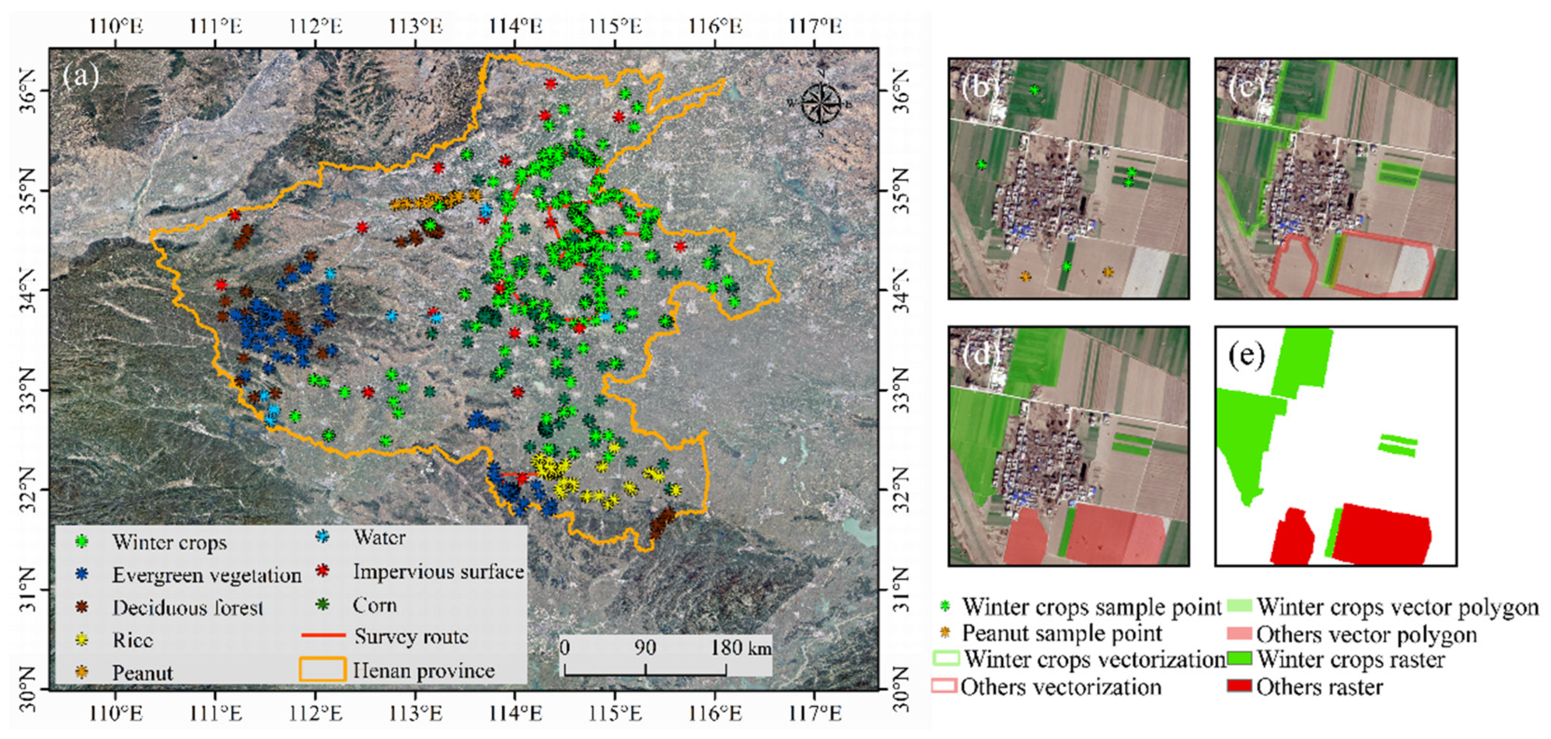
The main research ideas of this study are shown in Figure 1, mainly including 5 aspects: (1) Combine Landsat 7/8 and Sentinel 2A/B surface reflectance (SR) data to construct a high spatiotemporal resolution data set. (2) Calculate the index, including the normalized vegetation difference index (NDVI), land surface water index (LSWI), modified normalized difference water index (mNDWI) and enhanced vegetation index (EVI). Time series reconstruction, including the 10 day composite, linear interpolation and Savitzky–Golay filter smoothing. (3) Generate annual map of land type in 2019. (4) Generate annual map of winter crops in 2019. (5) Accuracy assessment and comparison.

2.1. Study Area

Henan province is located in the central region of China and consists of 17 cities, covering an area of 167,000 km² (110°E~116°E, 31°N~36°N; Figure 2a). The south and west are mountains, and the rest are plains. Suitable temperatures and wide plains provide an excellent growth environment for crops (Figure 2b). Among them, arable land accounts for 68.2% of the province’s land area. The main crops are wheat, corn, garlic, rape and cotton, etc. According to the China Statistical Yearbook issued by the National Bureau of Statistics of China, Henan province has had the largest area of sown winter crops in the past five years in the country. In 2018, the planting area of winter crops in Henan province reached 57,399 km² (Figure 2a). Study of China’s largest province for growing winter crops will help to obtain better planting information and seasonal dynamics of winter crops.

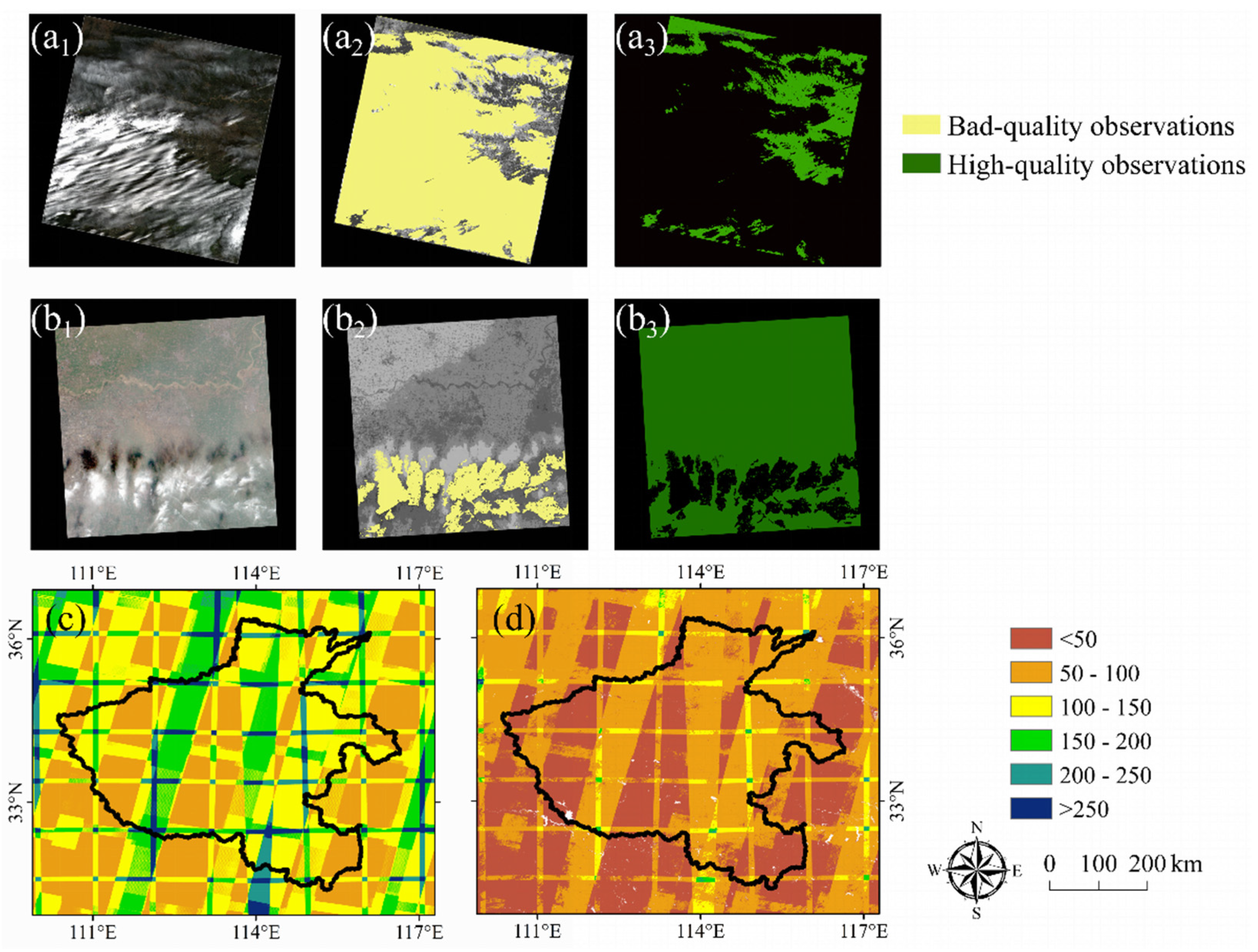
2.2. Datasets and Preprocessing

2.2.1. Landsat and Sentinel-2 Data

Landsat 7/8 were launched in April 1999 and February 2013 respectively, carrying the Enhanced Thematic Mapper (ETM+) and Operational Land Imager (OLI), with a 30 m spatial resolution and a single satellite revisit cycle of 15 days [46]. Sentinel-2 consists of two satellites, launched in June 2015 (Sentinel-2A) and March 2017 (Sentinel-2B), carrying the Multispectral Instrument (MSI) with a spatial resolution of 10 m, 20 m and 60 m, and the revisit cycle of the two satellites is 5 days [47]. The Google Earth Engine provides free top of atmosphere (TOA) reflectance data and atmospherically corrected SR data. Due to land surface changes, TOA data is not as sensitive as SR data [48]. We used all the available Landsat 7/8 and Sentinel-2A/B SR data for Henan Province during the research period as the initial image set. The data used is from the GEE cloud platform “Landsat/LE07/C01/T1_SR”, “Landsat/LC08/C01/T1_SR”, and “COPERNICUS/S2_SR”.

The detection of clouds and cloud shadows is essential for optical remote sensing data processing. First, we used the Fmask algorithm to detect poor quality observations in Landsat 7/8 images in GEE [49,50]. This method recognizes potential cloud pixels based on the physical properties of the cloud, detects cloud shadows through the darkening effect of the NIR band, and generates bad-quality observation masks by matching clouds and cloud shadows (Figure 3a). Second, we used the quality bands in the metadata to identify bad-quality observations in Sentinel-2A/B in GEE [8]. The metadata identifies those observations containing cirrus clouds and opaque clouds as bad-quality observations, and stores them as NODATA in the image, to generate a bad-quality observation mask (Figure 3b).

Due to the differences in the sensors in orbit, space and spectral configuration, the physical measurement value and radiation properties of the images will be affected [51], and the wavelength of each sensor can be slightly different; hence, it is necessary to normalize the remote sensing reflectance data to obtain comparable results. We used an ordinary least square regression coefficient to convert the ETM+ and MSI bands to the OLI bands standard. The five bands that needed to be processed are ${\rho }_{BLUE}$, ${\rho }_{GREEN}$, ${\rho }_{RED}$, ${\rho }_{NIR}$ and ${\rho }_{SWIR}$. The regression coefficients of the five bands we calculated are 0.8707, 0.8707, 0.9175, 0.9281, 0.9414 for ETM+ and 0.8729, 0.9621, 0.9103, 0.9701, 0.9668 for MSI [52,53].

In this study, a complete phenological period of winter crops was taken, and the date range was from 9/1/2018 to 9/1/2019. We collected a total of 3770 images from multiple sensors in Henan province during the study period. After removing the bad-quality observations following the process above, the total image numbers and high-quality image numbers of the Landsat and Sentinel per pixel are displayed in Figure 3c,d, respectively. Due to the long growing season length for winter crops, we counted available images for the study and high-quality observations per pixel in different periods. The specific details are shown in

Table 1. Number of images available and the number of observations per pixel at different periods.

Period	Image Number	Average Total Number of Observations Per Pixel	Average High-Quality Number of Observations Per Pixel
Before winter (September to December)	142	10	7
Overwintering period (December to February)	693	23	10
Greening period and harvest period (February to June)	1675	47	21
After harvest (June to September)	1260	35	21
Whole period (September to September)	3770	115	59

.

2.2.2. Ground Reference Data

We obtained ground reference data as training samples and verification samples by distributing questionnaires, agrometeorological station data, Google Earth images, and field survey data. First, we sent a questionnaire to students living in rural areas of Henan University. The information collected included the sowing date, harvest date and planting area of winter crops. Secondly, we collected data on crop phenology from the Henan agrometeorological station. The agrometeorological station recorded the dates of all the phenological events of winter crops from the sowing period to the harvest period. We used these data to compare with the phenological indicators map generated in this study to check consistency. Third, a satellite image from Google Earth images (including CNES/Airbus, Maxar Technologies, etc. satellite images) with a 1 m spatial resolution clearly shows the surface characteristics of cultivated land, rivers, roads and village buildings. We visually interpreted Google images to obtain the growing information of winter crops on cropland. Fourth, we conducted three field investigations in Henan province. During the investigation, we collected georeferenced photos containing different crop types. These field photos include common crop types such as winter crops, deciduous forests, evergreen forests, rice, corn, and peanuts. We collected a total of 329 winter crops fields and 288 non-winter-crops fields (60 in evergreen forest, 48 in deciduous forest, 82 in corn, 44 in rice, 27 in peanuts, 18 in impervious surface and 9 in water), and built time series of these fields.

2.2.3. Winter Crops Area from Statistical Yearbook

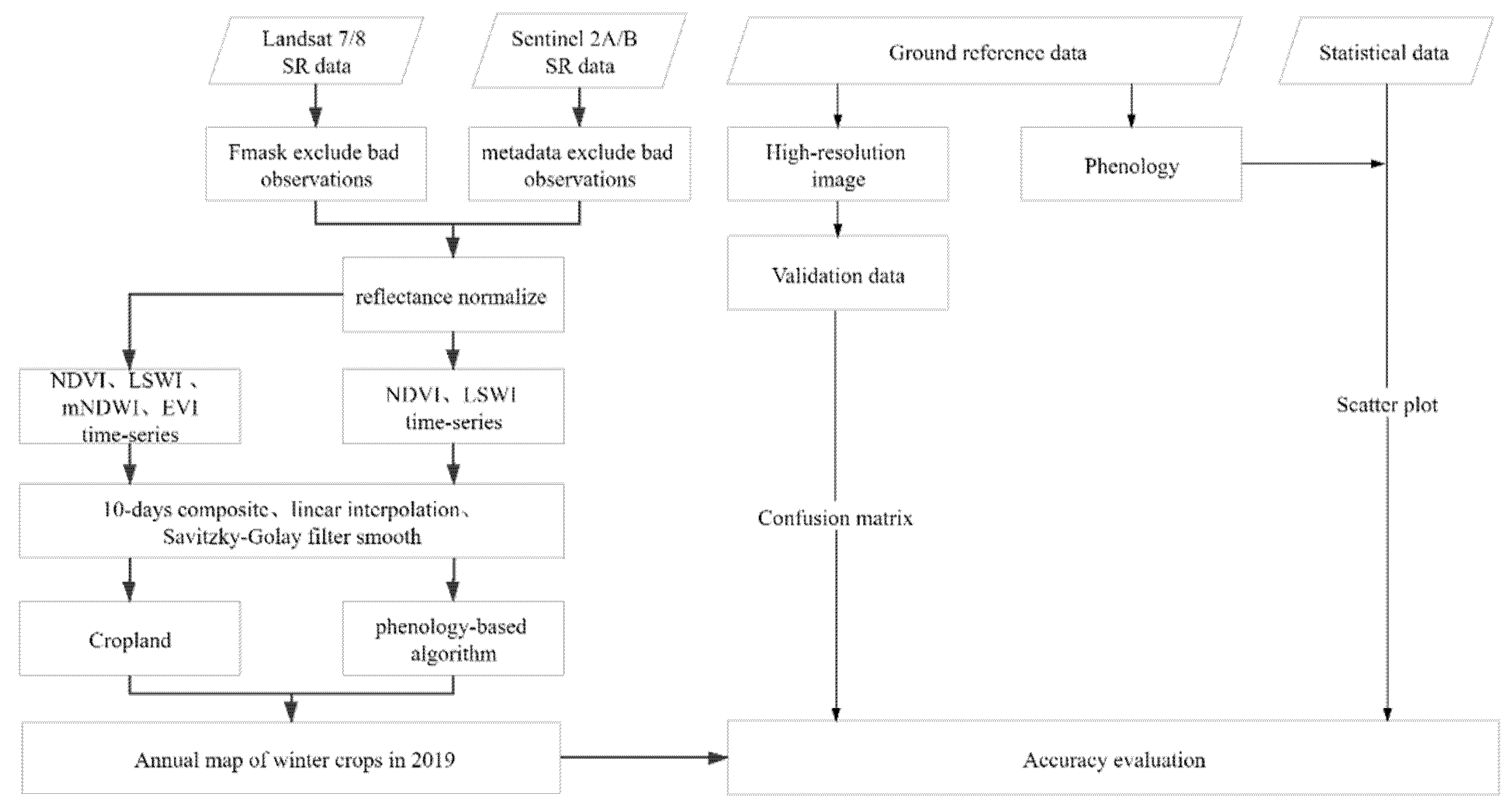
We collected the city-level and county-level statistical data in the Henan Provincial Statistical Yearbook in 2019 to compare with the results obtained by remote sensing methods. Although there are some problems with these data (statistical data may be overestimated due to false reports by farmers), national statistics are already the most trusted source of data on crop planting areas [30]. We selected a total of 17 prefecture-level cities, including 102 counties. The data can be obtained at https://data.cnki.net/yearbook/Single/N2020020050, 18 October 2020.

2.3. Methods

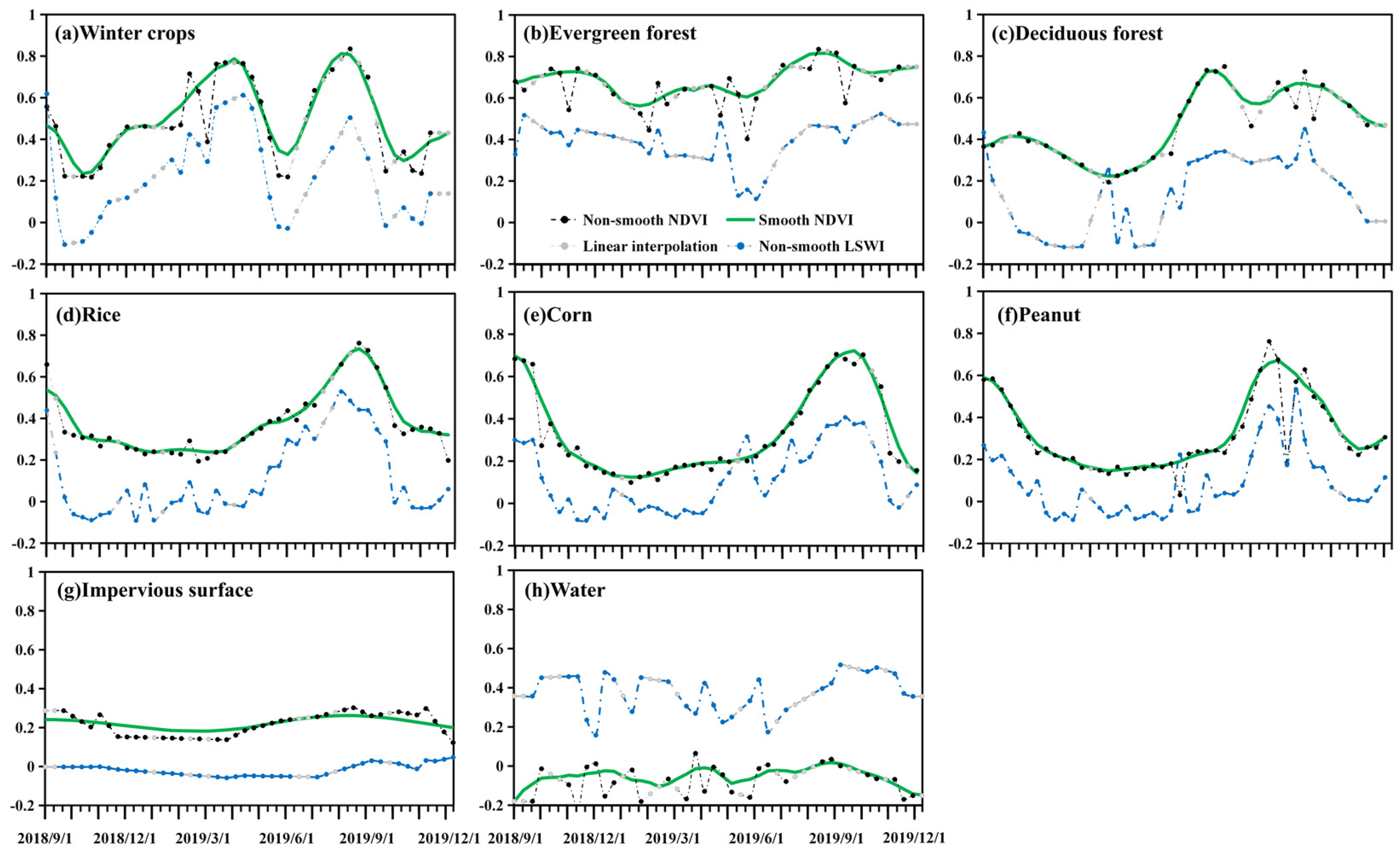
2.3.1. Index Calculation and Time-Series Processing

A normalized difference vegetation index (NDVI) time-series curve is a common and effective method to identify crops [54,55]. A land surface water index (LSWI) is used to assist identification of the start and end growth stages of winter crops [8,30]. In this study, a modified normalized difference water index (mNDWI) and enhanced vegetation index (EVI) were also calculated to extract different land cover types [56,57,58,59]. The calculation formulas are as follows:

$$NDVI=\frac{{\rho }_{NIR}-{\rho }_{RED}}{{\rho }_{NIR}+{\rho }_{RED}}$$

(1)

$$LSWI=\frac{{\rho }_{NIR}-{\rho }_{SWIR}}{{\rho }_{NIR}+{\rho }_{SWIR}}$$

(2)

$$mNDWI=\frac{{\rho }_{GREEN}-{\rho }_{SWIR}}{{\rho }_{GREEN}+{\rho }_{SWIR}}$$

(3)

$$EVI=2.5\times \frac{{\rho }_{NIR}-{\rho }_{RED}}{{\rho }_{NIR}+6\times {\rho }_{RED}-7.5\times {\rho }_{BLUE}+1}$$

(4)

where ${\rho }_{NIR}$ and ${\rho }_{RED}$ represent the near infrared band reflectance values and the red band reflectance values, respectively; ${\rho }_{SWIR}$ represents the shortwave infrared band reflectance values;${\rho }_{GREEN}$ represents the green band reflectance values; and ${\rho }_{BLUE}$ represents the blue band reflectance values.

The temporal resolutions, land surface coverages, and overlaps of the images obtained from the different sensors are different. In order to obtain an imagery set of the time series with equal intervals, we calculated the maximum value of NDVI and the average value of LSWI obtained every 10 days to develop a 10-day composite image [29,60]. If an image was affected by clouds, snow or other factors in some areas and good-quality observations within 10 days could not be obtained [30], we filled the time-series data set through linear interpolation based on good-quality observations before and after 10 days [61,62]. Even if the above data set is strictly preprocessed, there are still noises caused by cloud residues, data transmission errors, biological directional effects, or ice/snow cover [63]. We used a Savitzky–Golay filter (S–G filter) to smooth the time-series curves, reducing noise and constructing a good-quality NDVI time-series data set [64].

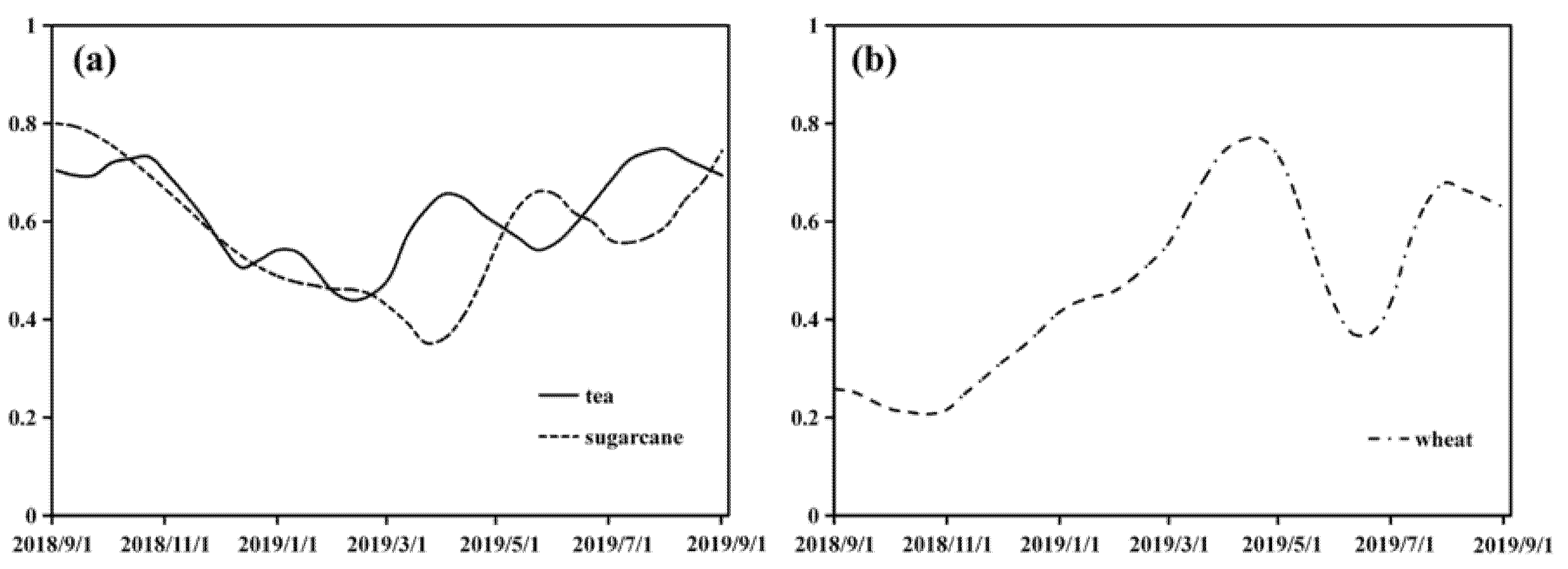
2.3.2. NDVI and LSWI Time Series Construction

We selected six types of vegetation sample points from winter crops, evergreen forests, deciduous forests, rice, corn, and peanuts from the surface reference data and created NDVI and LSWI time series at these points. The time series obtained by 10-day composite, linear interpolation and S–G filter reconstruction can truly reflect the vegetation growth status (Figure 4a–f). In addition, in order to obtain a mask containing only croplands, we also selected sample points of impervious surfaces and water (Figure 4g–h). Since the growth period of most crops is greater than 90 days, we used a moving window of 9 observations and a second-order filter to smooth the NDVI time series (LSWI is sensitive to water and soil moisture, so the LSWI time series data is not smoothed) [30].

2.3.3. Annual Maps of Croplands and Other Land Cover Types in 2019

To reduce the influence of other land cover types on our result, this study classified the land cover of the study area to obtain the cropland mask. We classified the land into four types: forest, impervious surface, water and cropland. Samples of different land cover types were obtained from ground reference data, among which 60 were evergreen forests, 48 were deciduous forests, 18 were impervious surface and 9 were water. Time-series curves were generated using these sample points and standard deviations were calculated (Figure 5). First, we identified the forest. In the study area, forests usually include evergreen forests and deciduous forests. A variety of forest identification methods have been developed [65,66,67]. As shown in Figure 5a,b, we developed a new model based on LSWI and EVI to identify forests. The number of pixel observations with LSWI > 0 and EVI > 0.2 exceeds 50% in a year were identified as forest pixels, and the forest pixels with a median NDVI (from November 1 to December 31) greater than 0.7 were identified as evergreen forest (Figure 5(a₁,a₂,a₄)), the forest pixels with a maximum NDVI (April 10 to May 20) greater than 0.5 were identified as deciduous forest (Figure 5(b₁,b₂,b₄)). Second, we identified impervious surfaces. The SWIR band of impervious pixels is usually larger than the NIR band, which makes LSWI a negative value [8]. We extracted impervious surfaces based on this feature, and the number of observations with a pixel’s LSWI less than 0 in a year exceeded 90% of the total number of observations in that year (Figure 5(c₂)). Third, we extracted water. If there were more than 80% of observations in which mNDWI was greater than NDVI, or mNDWI was greater than EVI, and EVI was less than 0.1 (Figure 5(d₁,d₃,d₄)), then this pixel was determined as water [68]. Finally, we used the pixels outside these three types of land as croplands pixels for the next step of analysis. The specific operations are summarized in

Table 2. Summary of the phenology based algorithms to generate the main noncropland land cover types in the study area.

Land Cover Types	Subset	Methods	References
Forest	Evergreen	LSWI>0 and EVI > 0.2, Freq > 50%, and NDVI_median > 0.7(November 1 to December 31)	[65,66,67]
	Deciduous	LSWI > 0 and EVI > 0.2, Freq > 50%, and NDVI_max > 0.5(April 10 to May 20)
Impervious surface	/	LSWI < 0, Freq > 90%	[8]
Water	/	mNDWI > NDVI or mNDWI > EVI, and EVI < 0.1, Freq > 80%	[68]

.

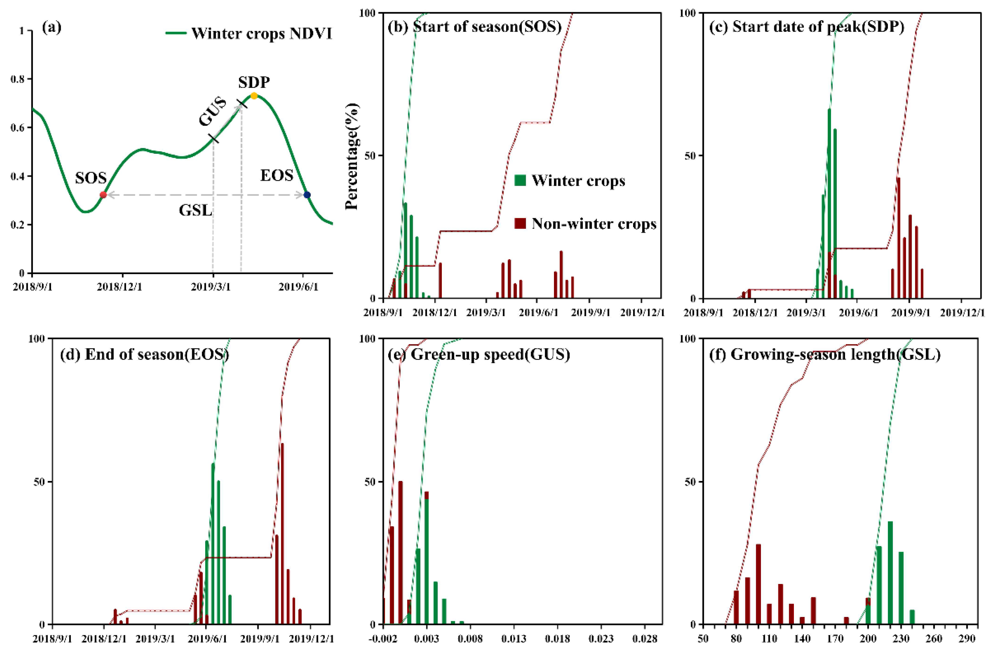
2.3.4. Annual Map of Winter Crops in 2019

Figure 4 shows the time-series curves of NDVI after the reconstruction and the LSWI time series of the different types of vegetation in the Henan province. The figure shows a significant difference between the curve shapes of winter crops and other vegetation. Winter crops are sown in mid-to-late October. At this time, NDVI gradually increases and stops growing in winter. After returning to green from February to March, it enters a rapid greening period, and NDVI increases rapidly, reaching its peak growth period from April to May, when NDVI reaches its peak. After that, the NDVI gradually declines, as it matures and harvests from June to July. The NDVI falls to a valley again, when the growth cycle of winter crops ends. Based on the information obtained above, the phenological indicators we extracted for classification are the start of season (SOS), the start date of peak (SDP), the end of season (EOS), the green-up speed (GUS) and the growing season length (GSL) (Figure 6a). In this study, we combined the peak and valley of the NDVI time series, the local minimum of the LSWI time series and the NDVI threshold method to calculate SOS, SDP and EOS. The GUS was calculated by the ratio of the NDVI change to the date span between the rapid greening period and the peak period, and the difference between EOS and SOS was used to calculate GSL. The specific steps were as follows:

Step 1: Identification of the peaks and valleys in the NDVI time series. Based on the NDVI time series, the algorithm was iterated on the pixels. When the value at a certain moment in the time series was greater (less) than its previous value and the next value, it was defined as the peak (valley), and the peak and valley troughs on each pixel were stored in the form of DOY (day of year).

Step 2: Filtering all the peaks and valleys obtained. For peaks, set the threshold to 0.6 to remove extra peaks caused by weeds or incomplete harvesting [69]. For valleys, the valleys with an LSWI greater than 0 were removed [67].

Step 3: Determining the date when SOS, SDP and EOS occurred [70]. In this study, we used a method of continuously detecting the emergence and growth of crops throughout the winter crops growth cycle, and determined the SOS and EOS of winter crops by calculating the maximum rate of NDVI changes [71]. The formula is as follows:

$$NDV{I}_{ratio}=\frac{NDVI-NDV{I}_{min}}{NDV{I}_{max}-NDV{I}_{min}}$$

(5)

where the $NDV{I}_{max}$ and $NDV{I}_{min}$ represent the maximum value and minimum value of NDVI from September 1, 2018 to June 30, 2019. From the emergence of crops, $NDV{I}_{ratio}$ increases with the increase of the crop $NDVI$ value. The moments when $NDV{I}_{ratio}$ is 0 and 1, respectively, represent the bare soil period and the SDP in the time series. In this study, SOS was defined as the DOY when $NDV{I}_{ratio}$ increased to 0.1 for the first time, EOS was defined as the DOY when $NDV{I}_{ratio}$ decreased to 0.18 for the first time [72], and SDP was defined as the DOY when the peak occured. Through the above steps, we have obtained SOS, SDP and EOS on pixel.

Step 4: The calculation formulas of green-up speed (GUS) and growing-season length (GSL) are as follows:

$$GUS=\frac{NDV{I}_{peak}-NDV{I}_{revive}}{DO{Y}_{peak}-DO{Y}_{revive}}$$

(6)

$$GSL=\mathrm{EOS}+365-\mathrm{SOS}$$

(7)

where $NDV{I}_{peak}$ and $NDV{I}_{revive}$ represent the NDVI peak value during the whole growth cycle and the first NDVI value when the revive period began, respectively; $DO{Y}_{peak}$ and $DO{Y}_{revive}$ represent the date when these two values occurred; in this study, the revive period was defined as 3/1/2019. GUS was defined as the average daily increase speed of NDVI during the revive period. GSL was defined as the time span from SOS to EOS.

Step 5: We calculated phenological indicators at these sample points using winter crop samples and nonwinter crop samples in the ground reference data, as shown in Figure 6b–f.

Step 6: Based on the phenological information provided by these sample points, we found that SOS for winter crops usually occurs from early October to early November, SDP occurs between late March and early May, and EOS occurs between late May and early July. In the rapid greening period, the daily growth rate of NDVI exceeds 0.001, and the date span of the complete growth cycle is more than 200 days. Based on the information of these phenological indicators, we developed a decision classification approach of 260 < SOS < 330, 80 < SDP < 140, 130 < EOS < 190, GUS > 0.001, 200 < GSL < 250.

Step 7: Algorithms were performed on the scale of the pixels, and the annual map of winter crops in the Henan province in 2019 was generated.

2.3.5. Accuracy Evaluation

We used a confusion matrix for accuracy evaluation. Section 2.2.2 introduced the process of obtaining ground reference data. The spatial distribution of samples is shown in Figure 7a. We used the coordinate information and area information of these sample to locate them in the Google Earth high-resolution image, combined with field photos and survey data to generate verification data for the calculation of the confusion matrix, and finally obtained the number of winter crop polygons used for verification as 329 (17,475 pixels), and the number of other polygons was 288 (12,739 pixels). The specific process was as follows:

(1) The coordinates of the sample we collected were located in the Google Earth image. Due to the high resolution of the Google Earth image, the boundary of the field was clearly identified (Figure 7b).

(2) Vectorization. The size of each vector boundary depends on the size of the field where the sample is located. Through visual interpretation, we determined the shape of the field, drew the vector boundary of the field (Figure 7c), and then converted the vector boundary into a vector polygon (Figure 7d).

(3) Converted the vector polygon to raster data (Figure 7e) and used bicubic resampling to resample the raster data to 30 m.

(4) Generated the confusion matrix, compared the manually, visually interpreted raster data with the classification results in this study, and calculated the user’s accuracy, producer’s accuracy, overall accuracy and Kappa coefficient.

We also used winter crop phenology observations from the 51 agrometeorological stations and the statistical data of cities and counties in the Henan Provincial Statistical Yearbook 2019 to compare with the results of this study, and calculated R² and Root Mean Square Error (RMSE) to assess its relevance.

3. Results

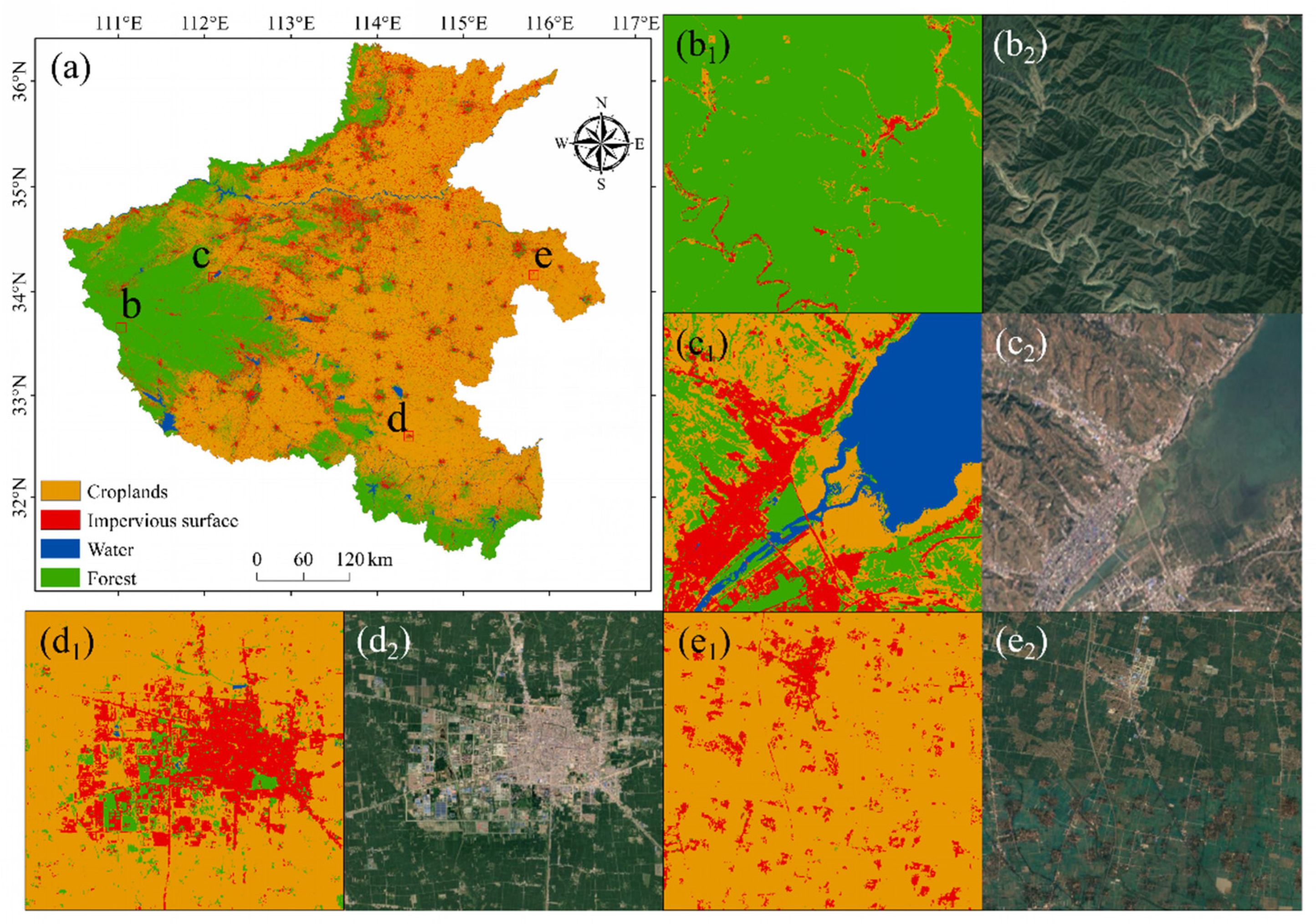
3.1. Annual Maps of Croplands and Other Land Cover Types in 2019

We used the algorithm introduced in Section 2.3.3 to generate a 30 m land cover types map of Henan province in 2019, including forests, impervious surfaces, water, and croplands (Figure 8). The croplands cover an area of 107,573.02km², accounting for 64.41% of the total area. We removed the three types of pixels of forests, impervious surface and water to obtain the croplands mask. The next step of the algorithm was performed on the cropland pixels.

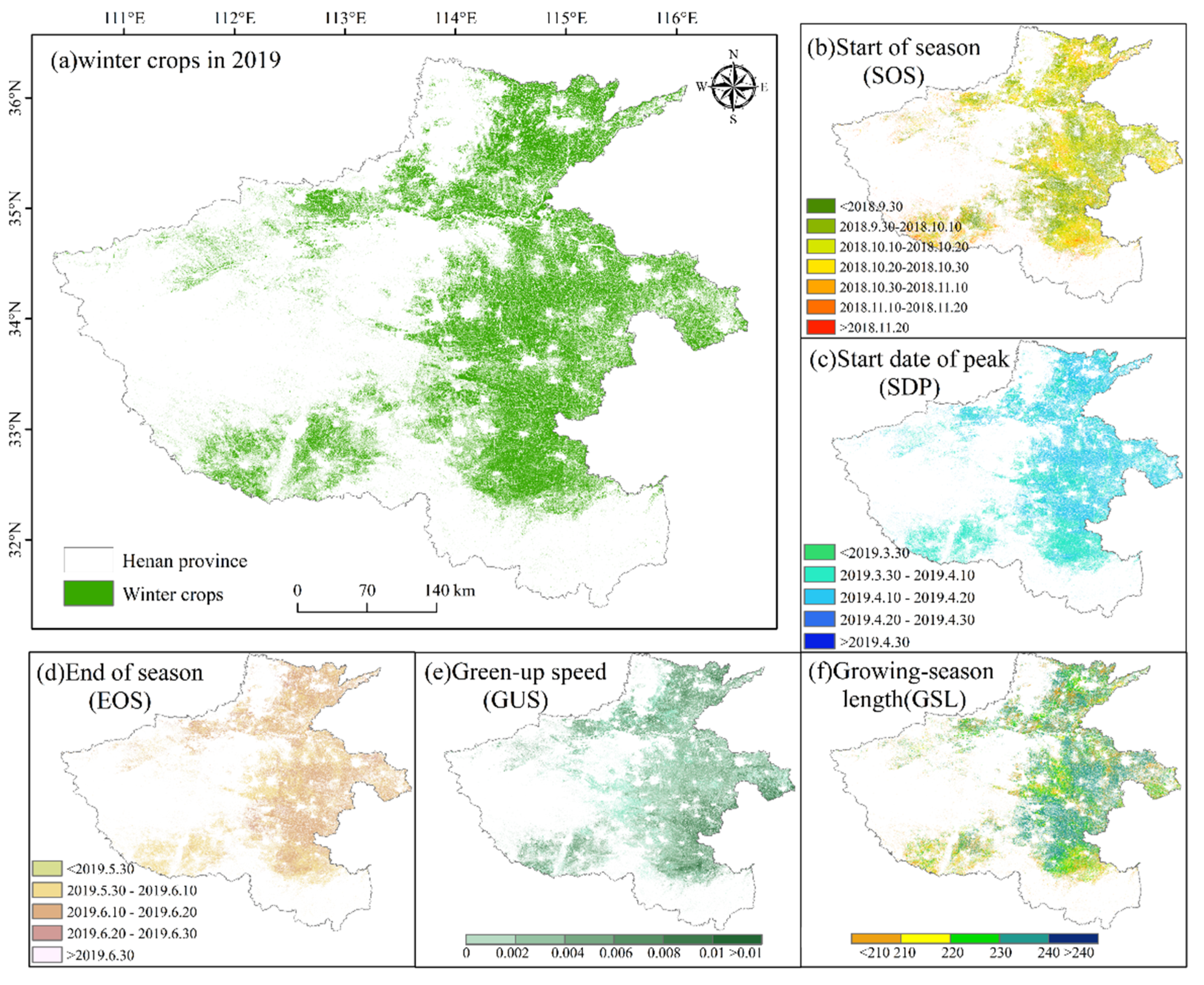
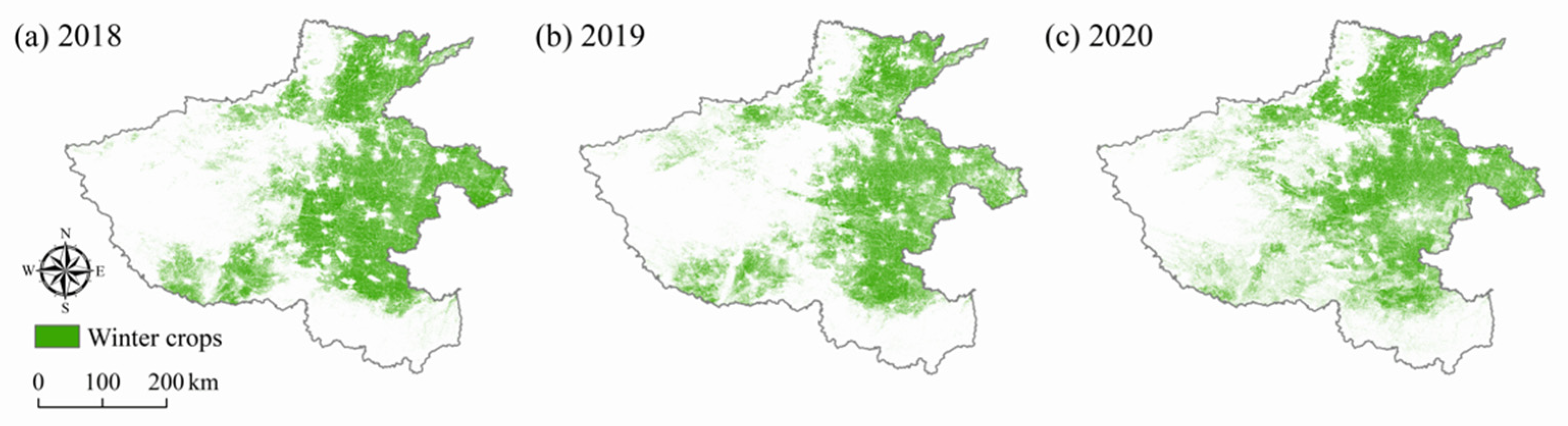
3.2. Annual Map of Winter Crops in 2019

The resultant annual map of winter crops in the Henan province is shown in Figure 9a, with a total area of 44,407.4km². The main planting areas of winter crops are the central and eastern plains of study area. The distribution of winter crops in the southwest and western mountain areas is relatively small. The blank spaces in the study area are mainly urban areas, single-season crop areas (such as Xinyang, which mostly sows single spring rice).

Figure 9b–f, respectively, show the start of season, start date of the peak, end of season, green-up speed and growing-season length of winter crops in Henan province. We believe that the purpose of the phenological indicator map lies in the fact that although these phenological indicators show the spatial distribution and no significant trend of latitude or longitude, it can provide policy makers with information on winter crop cultivation to develop food production and food security policies. It can also provide winter crop phenological characteristics and seasonal dynamics to contractors, food manufacturers or farmers for better management of winter crop growth processes. In general, the phenological indicators map in this study provides reference for the phenological monitoring of the whole growing season of winter crops, and can be used to predict the planting situation of the land in the next year.

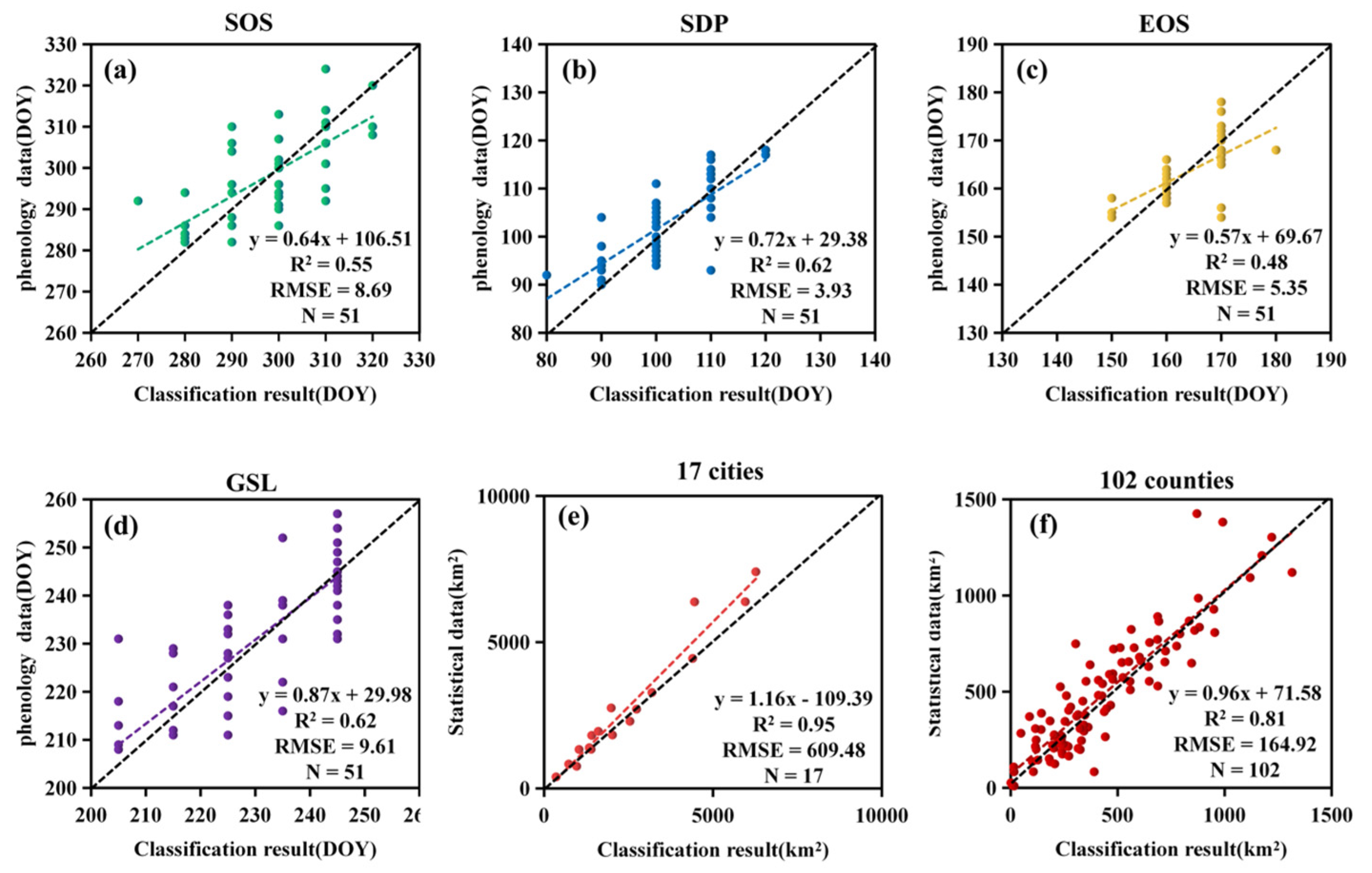
3.3. Accuracy Assessment and Comparison of the 2019 Winter Crops Map

The accuracy of the winter crops distribution map in 2019 was evaluated using the raster obtained in Section 2.3.5. Based on the raster data converted from 329 winter crop vector polygons (17,475 pixels) and 288 nonwinter crop vector polygons (12,739 pixels), the accuracy evaluation results using the confusion matrix are shown in

Table 3. Accuracy assessment based on the ground reference data for winter crops and others in 2019. This table shows the user’s (UA), producer’s (PA) and overall (OA) accuracy.

Class	Error Matrix (Pixel/km2)			Accuracy (%)
	Winter Crops	Others	Total	User’s	Producer’s	Overall
Winter Crops	16,883/15.19	1,052/0.95	17,935/16.14	96.61	94.13	94.56
Others	592/0.53	11,687/10.52	12,279/11.05	91.74	95.18
Total	17,475/15.72	12,739/11.47	30,214/27.19	/	/	/

. The user accuracy, producer accuracy and total accuracy of the model were 96.61%, 94.13% and 94.56%, respectively, showing a high classification accuracy. The Kappa coefficient was 0.89, indicating that there is a strong consistency between the ground reference data and classification results. Figure 10 is a comparison between the ground reference data after visual interpretation and the classification results. The selected area is a rectangular area containing typical ground objects. The error shows that the commission of winter crops is mainly concentrated on the cropland road network. This is because the width of rural roads is generally less than 30 m, and the 30 m spatial resolution data set constructed in this study was generally unable to identify such linear ground objects. The omission classification of winter crops is mainly concentrated around the village buildings, and the irregularity of the village boundary makes it impossible to correctly identify the small planting areas of winter crops embedded around the buildings.

We used 51 phenology data from the Henan agrometeorological station and statistical data (17 cities and 102 counties) in Henan province in 2019 to compare with the classification results in this study. As the data provided by the agrometeorological station only includes the seedling stage (when winter crops begin to grow), heading stage (when winter crops reach the maximum growth period) and harvest stage (when winter crops are harvested after maturity), there is no GUS and GSL. We defined crop seedling as SOS, heading stage as SDP, harvest as EOS, and the GSL was defined by the time span of the seedling stage to mature stage. The data obtained are compared with the phenological indicators of this study (Figure 11a–d). R² was between 0.48~0.62, and RMSE between 3.93~9.61. Figure 11e,f show the comparison between the statistical data (17 cities and 102 counties) and the classification results in this study, respectively. The total area of winter crops fields in Henan from the classification results is 44,407.4 km², which is 8.4% less than the area estimated (48,469.8 km²) from the statistical data. From the comparison of different levels, the statistical data of 11 cities and 66 counties are overestimated. R² is 0.95 and 0.81, RMSE is 609.48 and 164.92, respectively, showing significant correlation and consistency.

4. Discussion

4.1. Potential of Multi-Sensor for Agricultural Mapping

Annual cropland mapping methods for large scale crop monitoring must meet multiple requirements, such as timeliness, accuracy and cost-effectiveness. Following China’s implementation of the household contract responsibility system, the fields in the study area are small [73] and mixed with residential areas, roads, rivers and lakes. Classification results using low spatial resolution images (such as MODIS images) can be poor. The disadvantage of using high spatial resolution images (such as Landsat images) is that the revisit period is too long, resulting in an insufficient number of images available, which has a significant impact on the extraction of images in a specific period by the multitemporal method. High spatiotemporal resolution image acquisition is the first problem to be solved by agricultural remote sensing. Currently available high spatiotemporal resolution data, such as GaoFen satellite images, are difficult to acquire and the data acquisition cost is too high.

In this study, the combination of Landsat 7/8 and Sentinel-2A/B images greatly increased the number of high-quality observations of individual pixels, and the phenological indicators of winter crops were captured well by reconstructing the time resolution of the time series [63,70,71]. Through linear interpolation and S–G filtering, on the one hand, the continuity of the time series was maintained, on the other hand, this process overcomes the difficulty of extracting the complete original NDVI time-series curve from scattered data [74]. Through the above operations, we have obtained an image set with high spatiotemporal resolution. A sufficient number of images and high-quality observations make the classification results more scientific and accurate.

This paper only takes 2019 as an example of the extraction of the planting area of winter crops in Henan Province. GEE contains Landsat satellite databases for the past few decades and Sentinel satellite databases for the past few years, and is freely available. By using past images, our algorithm can also be used to extract winter crops in the desired year or region (Figure 12), which makes it possible to analyze the temporal and spatial changes of winter crops in a long-time series. The precondition is that the region studied should have images of sufficient quality and quantity.

4.2. Algorithm Improvement

Previous studies have proved the potential of large area mapping based on phenological algorithms [8,9,20,73,74]. The phenological periods selected are different, but they are closely related to the phenological changes that occur during the growth season. Based on previous studies on the phenological algorithm of winter crops, most studies have focused on a specific phenological period, such as the pre-winter peak (PBW) [32], peak growth period (PG) and peak drought period (PD) [40], greening period and withering period [16,38], etc. In fact, due to the long growth cycle of winter crops, phenological events similar to winter crops may also occur in other vegetation in a specific phenological period. For example, sugarcane generally has a small peak around May and tea in some areas has a peak in winter, both of which are the peak periods of winter crops (Figure 13a). The phenological indicators extracted in this study cover the whole growth season. Only the pixels that follow the decision classification of the five phenological indicators will be recognized as winter crop pixels, which reduces confusion. There is a study performed using crop proportion phenology index (CPPI) models by focusing on the whole growth season of winter crops [21]. The phenological indicators included the eigenvalues of seeding date, first peak, second peak and harvest date in the time series. Although the model studies multiple periods in the whole growth season, it requires winter crops to accurately provide two peaks. In a large range, due to differences in spatial distribution and the influence of different agricultural practices, winter crops in the growth cycle may show different time series; it may not be possible to obtain all the parameters required by the model (for example, in the central part of Henan province, the NDVI of winter crops reached its peak only at the heading stage, but not before winter) (Figure 13b).

The phenology based algorithm developed in this study focuses on the whole winter crop growth season. By determining five phenological indicators (SOS, SDP, EOS, GUS and GSL) and mapping on pixels, an effective, high precision winter crops identification and mapping algorithm was constructed. Compared with the above studies, our algorithm has the following improvements: (1) By analyzing the whole growth cycle of winter crops, the planting area of winter crops can be extracted more accurately. (2) The phenological indicators of different periods are extracted, which is conducive to monitoring the winter crops planting information and seasonal dynamics.

4.3. Uncertainty

To reduce the influence of other vegetation on the extraction of winter crops, we generated the annual land cover types map of Henan province in 2019 through the threshold method, but this may also lead to the omission of classification of winter crops. As the study area is large, there may be differences in the time-series curves of the same species with different spatial distributions, so the set threshold cannot be applied to the whole study area. For example, some winter crops have large NDVI values in winter, and the time window for extracting forests overlaps with the growth periods of winter crops. These conditions may cause cropland pixels to be classified as forest pixels, leading to the omission of winter crop planting areas. In addition, this study only classifies land into four types, and does not classify the map in detail. In the future, the accuracy can be improved by improving the threshold, comparing the size of the VI indexes with each other, or classifying the land into more types.

Due to the influence of clouds, it is difficult to guarantee that each pixel has a satellite image every 10 days. When an image is missing, the interpolation algorithm of adjacent pixels is adopted. This algorithm guarantees the time continuity of the data, but when the image is missing at the inflection point, the interpolation cannot reflect the true position of the crop growth, and there is a certain degree of uncertainty. Sentinel-1 data sets are suitable for high precision agricultural classification mapping due to its short revisit period and dual polarization channels, thus, images are not affected by weather and can be used to estimate the phenological period of crops [75,76]. In the correlation analysis in Section 3.3, we compared the phenological indicators extracted in this study with the phenological data from agrometeorological stations. R² is between 0.48 and 0.62. The main reason for the weak correlation is that the time interval set in this study is 10 days, and the data from the agrometeorological station is accurate to 1 day. In the future, the data set can be composited and interpolated at five days, two day or even one day time intervals to obtain a higher time resolution data set. In addition, winter crops include winter wheat, winter rapeseed and garlic. This study has not been subdivided. In the future, the optimization algorithm will be used to map several crops with the same growing season.

5. Conclusions

Based on the Google Earth Engine, all available Landsat 7/8 and Sentinel-2A/B images (3,770 scene images in total) during the study period were obtained. A simple, high-precision and low cost, phenology based algorithm was developed to generate an annual winter crop map in Henan province. The total accuracy was 94.56%, and the Kappa coefficient was 0.89. The conclusions of this study are as follows: (1) The combination of multiple sensor data to construct a high spatiotemporal resolution image collection significantly increases the number of high-quality image observations available on each pixel and better captures the phenology of winter crops. (2) The phenology based algorithm developed has been shown to have the potential to extract winter crops on a large scale. This study provides a scientific basis and reference case for crop extraction using phenological methods in other regions and types.

References

1. Franch, B.; Vermote, E.; Becker-Reshef, I.; Claverie, M.; Huang, J.; Zhang, J.; Justice, C.; Sobrino, J.A. Improving the timeliness of winter wheat production forecast in the United States of America, Ukraine and China using MODIS data and NCAR Growing Degree Day information. Remote Sens. Environ. 2015, 161, 131–148. [Google Scholar] [CrossRef]
2. Liming, W.; Liu, J.; Fugang, Y.; Changhong, F.; Fei, T.; Jianmeng, G. Early recognition of winter wheat area based on GF-1 satellite. Trans. Chin. Soc. Agric. Eng. 2015, 31, 194–201. [Google Scholar]
3. Shao, Y.; Campbell, J.B.; Taff, G.N.; Zheng, B. An analysis of cropland mask choice and ancillary data for annual corn yield forecasting using MODIS data. Int. J. Appl. Earth Obs. Geoinf. 2015, 38, 78–87. [Google Scholar] [CrossRef]
4. Jiao, X.; Kovacs, J.M.; Shang, J.; McNairn, H.; Walters, D.; Ma, B.; Geng, X. Object-oriented crop mapping and monitoring using multi-temporal polarimetric RADARSAT-2 data. ISPRS J. Photogramm. Remote Sens. 2014, 96, 38–46. [Google Scholar] [CrossRef]
5. Jin, Z.; Azzari, G.; Lobell, D.B. Improving the accuracy of satellite-based high-resolution yield estimation: A test of multiple scalable approaches. Agric. For. Meteorol. 2017, 247, 207–220. [Google Scholar] [CrossRef]
6. Frolking, S.; Qiu, J.; Boles, S.; Xiao, X.; Liu, J.; Zhuang, Y.; Li, C.; Qin, X. Combining remote sensing and ground census data to develop new maps of the distribution of rice agriculture in China. Glob. Biogeochem. Cycles 2002, 16, 38-1–38-10. [Google Scholar] [CrossRef] [Green Version]
7. Hao, W.; Mei, X.; Cai, X.; Du, J.; Liu, Q. Crop planting extraction based on multi-temporal remote sensing data in Northeast China. Trans. Chin. Soc. Agric. Eng. 2011, 27, 201–207. [Google Scholar]
8. Wang, J.; Xiao, X.; Liu, L.; Wu, X.; Qin, Y.; Steiner, J.L.; Dong, J. Mapping sugarcane plantation dynamics in Guangxi, China, by time series Sentinel-1, Sentinel-2 and Landsat images. Remote Sens. Environ. 2020, 247, 111951. [Google Scholar] [CrossRef]
9. Massey, R.; Sankey, T.T.; Congalton, R.G.; Yadav, K.; Thenkabail, P.S.; Ozdogan, M.; Meador, A.J.S. MODIS phenology-derived, multi-year distribution of conterminous US crop types. Remote Sens. Environ. 2017, 198, 490–503. [Google Scholar] [CrossRef]
10. Niu, W.; Xia, H.; Wang, R.; Pan, L.; Meng, Q.; Qin, Y.; Li, R.; Zhao, X.; Bian, X.; Zhao, W. Research on Large-Scale Urban Shrinkage and Expansion in the Yellow River Affected Area Using Night Light Data. ISPRS Int. J. Geo-Inf. 2021, 10, 5. [Google Scholar] [CrossRef]
11. Tassi, A.; Vizzari, M. Object-Oriented LULC Classification in Google Earth Engine Combining SNIC, GLCM, and Machine Learning Algorithms. Remote Sens. 2020, 12, 3776. [Google Scholar] [CrossRef]
12. Mulla, D.J. Twenty five years of remote sensing in precision agriculture: Key advances and remaining knowledge gaps. Biosyst. Eng. 2013, 114, 358–371. [Google Scholar] [CrossRef]
13. Pulwarty, R.S.; Sivakumar, M.V. Information systems in a changing climate: Early warnings and drought risk management. Weather Clim. Extrem. 2014, 3, 14–21. [Google Scholar] [CrossRef] [Green Version]
14. Wu, B.; Meng, J.; Li, Q.; Yan, N.; Du, X.; Zhang, M. Remote sensing-based global crop monitoring: Experiences with China’s CropWatch system. Int. J. Digit. Earth 2014, 7, 113–137. [Google Scholar] [CrossRef]
15. Wang, J.; Tian, H.; Wu, M.; Wang, L.; Wang, C. Rapid Mapping of Winter Wheat in Henan Province. J. Geo-Inf. Sci. 2017, 19, 846–853. [Google Scholar]
16. Qiu, B.; Luo, Y.; Tang, Z.; Chen, C.; Lu, D.; Huang, H.; Chen, Y.; Chen, N.; Xu, W. Winter wheat mapping combining variations before and after estimated heading dates. ISPRS J. Photogramm. Remote Sens. 2017, 123, 35–46. [Google Scholar] [CrossRef]
17. Liu, J.; Feng, Q.; Gong, J.; Zhou, J.; Liang, J.; Li, Y. Winter wheat mapping using a random forest classifier combined with multi-temporal and multi-sensor data. Int. J. Digit. Earth 2018, 11, 783–802. [Google Scholar] [CrossRef]
18. Wolanin, A.; Camps-Valls, G.; Gómez-Chova, L.; Mateo-García, G.; van der Tol, C.; Zhang, Y.; Guanter, L. Estimating crop primary productivity with Sentinel-2 and Landsat 8 using machine learning methods trained with radiative transfer simulations. Remote Sens. Environ. 2019, 225, 441–457. [Google Scholar] [CrossRef]
19. Tian, H.; Huang, N.; Niu, Z.; Qin, Y.; Pei, J.; Wang, J. Mapping Winter Crops in China with Multi-Source Satellite Imagery and Phenology-Based Algorithm. Remote Sens. 2019, 11, 820. [Google Scholar] [CrossRef] [Green Version]
20. Becker-Reshef, I.; Vermote, E.; Lindeman, M.; Justice, C. A generalized regression-based model for forecasting winter wheat yields in Kansas and Ukraine using MODIS data. Remote Sens. Environ. 2010, 114, 1312–1323. [Google Scholar] [CrossRef]
21. Pan, Y.; Li, L.; Zhang, J.; Liang, S.; Zhu, X.; Sulla-Menashe, D. Winter wheat area estimation from MODIS-EVI time series data using the Crop Proportion Phenology Index. Remote Sens. Environ. 2012, 119, 232–242. [Google Scholar] [CrossRef]
22. Skakun, S.; Franch, B.; Vermote, E.; Roger, J.-C.; Becker-Reshef, I.; Justice, C.; Kussul, N. Early season large-area winter crop mapping using MODIS NDVI data, growing degree days information and a Gaussian mixture model. Remote Sens. Environ. 2017, 195, 244–258. [Google Scholar] [CrossRef]
23. Huang, J.; Zhao, J.; Wang, X.; Xie, Z.; Wen, Z.; Ran, H. Extraction Method of Growth Stages of Winter Wheat Based on Accumulated Temperature and Remote Sensing Data. Trans. Chin. Soc. Agric. Mach. 2019, 50, 176–183. [Google Scholar]
24. Geerken, R.A. An algorithm to classify and monitor seasonal variations in vegetation phenologies and their inter-annual change. ISPRS J. Photogramm. Remote Sens. 2009, 64, 422–431. [Google Scholar] [CrossRef]
25. He, J.; Zhao, W.; Li, A.; Wen, F.; Yu, D. The impact of the terrain effect on land surface temperature variation based on Landsat-8 observations in mountainous areas. Int. J. Remote Sens. 2019, 40, 1808–1827. [Google Scholar] [CrossRef]
26. Gao, F.; Anderson, M.C.; Zhang, X.; Yang, Z.; Alfieri, J.G.; Kustas, W.P.; Mueller, R.; Johnson, D.M.; Prueger, J.H. Toward mapping crop progress at field scales through fusion of Landsat and MODIS imagery. Remote Sens. Environ. 2017, 188, 9–25. [Google Scholar] [CrossRef] [Green Version]
27. Torbick, N.; Chowdhury, D.; Salas, W.; Qi, J. Monitoring rice agriculture across myanmar using time series Sentinel-1 assisted by Landsat-8 and PALSAR-2. Remote Sens. 2017, 9, 119. [Google Scholar] [CrossRef] [Green Version]
28. Defourny, P.; Bontemps, S.; Bellemans, N.; Cara, C.; Dedieu, G.; Guzzonato, E.; Hagolle, O.; Inglada, J.; Nicola, L.; Rabaute, T. Near real-time agriculture monitoring at national scale at parcel resolution: Performance assessment of the Sen2-Agri automated system in various cropping systems around the world. Remote Sens. Environ. 2019, 221, 551–568. [Google Scholar] [CrossRef]
29. Griffiths, P.; Nendel, C.; Hostert, P. Intra-annual reflectance composites from Sentinel-2 and Landsat for national-scale crop and land cover mapping. Remote Sens. Environ. 2019, 220, 135–151. [Google Scholar] [CrossRef]
30. Liu, L.; Xiao, X.; Qin, Y.; Wang, J.; Xu, X.; Hu, Y.; Qiao, Z. Mapping cropping intensity in China using time series Landsat and Sentinel-2 images and Google Earth Engine. Remote Sens. Environ. 2020, 239, 111624. [Google Scholar] [CrossRef]
31. Pan, L.; Xia, H.; Yang, J.; Niu, W.; Wang, R.; Song, H.; Guo, Y.; Qin, Y. Mapping cropping intensity in Huaihe basin using phenology algorithm, all Sentinel-2 and Landsat images in Google Earth Engine. Int. J. Appl. Earth Obs. Geoinf. 2021, 102, 102376. [Google Scholar] [CrossRef]
32. Tao, J.-B.; Wu, W.-B.; Yong, Z.; Yu, W.; Jiang, Y. Mapping winter wheat using phenological feature of peak before winter on the North China Plain based on time-series MODIS data. J. Integr. Agric. 2017, 16, 348–359. [Google Scholar] [CrossRef] [Green Version]
33. Li, F.; Ren, J.; Wu, S.; Zhao, H.; Zhang, N. Comparison of Regional Winter Wheat Mapping Results from Different Similarity Measurement Indicators of NDVI Time Series and Their Optimized Thresholds. Remote Sens. 2021, 13, 1162. [Google Scholar] [CrossRef]
34. Gao, H.; Wang, C.; Wang, G.; Li, Q.; Zhu, J. A new crop classification method based on the time-varying feature curves of time series dual-polarization Sentinel-1 data sets. IEEE Geosci. Remote Sens. Lett. 2019, 17, 1183–1187. [Google Scholar] [CrossRef]
35. Yang, Y.; Tao, B.; Ren, W.; Zourarakis, D.P.; Masri, B.E.; Sun, Z.; Tian, Q. An improved approach considering intraclass variability for mapping winter wheat using multitemporal MODIS EVI images. Remote Sens. 2019, 11, 1191. [Google Scholar] [CrossRef] [Green Version]
36. Dong, Q.; Chen, X.; Chen, J.; Zhang, C.; Liu, L.; Cao, X.; Zang, Y.; Zhu, X.; Cui, X. Mapping Winter Wheat in North China Using Sentinel 2A/B Data: A Method Based on Phenology-Time Weighted Dynamic Time Warping. Remote Sens. 2020, 12, 1274. [Google Scholar] [CrossRef] [Green Version]
37. Xia, H.; Qin, Y.; Feng, G.; Meng, Q.; Cui, Y.; Song, H.; Ouyang, Y.; Liu, G. Forest phenology dynamics to climate change and topography in a geographic and climate transition zone: The Qinling mountains in Central China. Forests 2019, 10, 1007. [Google Scholar] [CrossRef] [Green Version]
38. Zhang, X.; Shuai, T.; Yang, H.; Huang, C. Winter wheat planting area extraction based on MODIS EVI image time series. Trans. Chin. Soc. Agric. Eng. 2010, 26, 220–224. [Google Scholar]
39. Waldner, F.; Canto, G.S.; Defourny, P. Automated annual cropland mapping using knowledge-based temporal features. ISPRS J. Photogramm. Remote Sens. 2015, 110, 1–13. [Google Scholar] [CrossRef]
40. Wang, C.; Fan, Q.; Li, Q.; SooHoo, W.M.; Lu, L. Energy crop mapping with enhanced TM/MODIS time series in the BCAP agricultural lands. ISPRS J. Photogramm. Remote Sens. 2017, 124, 133–143. [Google Scholar] [CrossRef] [Green Version]
41. Lin, C.; Liu, Q.-S.; Huang, C.; Liu, G.-H. Monitoring of winter wheat distribution and phenological phases based on MODIS time-series: A case study in the Yellow River Delta, China. J. Integr. Agric. 2016, 15, 2403–2416. [Google Scholar]
42. Tamiminia, H.; Salehi, B.; Mahdianpari, M.; Quackenbush, L.; Adeli, S.; Brisco, B. Google Earth Engine for geo-big data applications: A meta-analysis and systematic review. ISPRS J. Photogramm. Remote Sens. 2020, 164, 152–170. [Google Scholar] [CrossRef]
43. Kumar, L.; Mutanga, O. Google Earth Engine applications since inception: Usage, trends, and potential. Remote Sens. 2018, 10, 1509. [Google Scholar] [CrossRef] [Green Version]
44. Chen, B.; Xiao, X.; Li, X.; Pan, L.; Doughty, R.; Ma, J.; Dong, J.; Qin, Y.; Zhao, B.; Wu, Z. A mangrove forest map of China in 2015: Analysis of time series Landsat 7/8 and Sentinel-1A imagery in Google Earth Engine cloud computing platform. ISPRS J. Photogramm. Remote Sens. 2017, 131, 104–120. [Google Scholar] [CrossRef]
45. Gorelick, N.; Hancher, M.; Dixon, M.; Ilyushchenko, S.; Thau, D.; Moore, R. Google Earth Engine: Planetary-scale geospatial analysis for everyone. Remote Sens. Environ. 2017, 202, 18–27. [Google Scholar] [CrossRef]
46. Wulder, M.A.; Masek, J.G.; Cohen, W.B.; Loveland, T.R.; Woodcock, C.E. Opening the archive: How free data has enabled the science and monitoring promise of Landsat. Remote Sens. Environ. 2012, 122, 2–10. [Google Scholar] [CrossRef]
47. Torres, R.; Snoeij, P.; Geudtner, D.; Bibby, D.; Davidson, M.; Attema, E.; Potin, P.; Rommen, B.; Floury, N.; Brown, M. GMES Sentinel-1 mission. Remote Sens. Environ. 2012, 120, 9–24. [Google Scholar] [CrossRef]
48. Jin, Z.; Azzari, G.; You, C.; Di Tommaso, S.; Aston, S.; Burke, M.; Lobell, D.B. Smallholder maize area and yield mapping at national scales with Google Earth Engine. Remote Sens. Environ. 2019, 228, 115–128. [Google Scholar] [CrossRef]
49. Foga, S.; Scaramuzza, P.L.; Guo, S.; Zhu, Z.; Dilley, R.D., Jr.; Beckmann, T.; Schmidt, G.L.; Dwyer, J.L.; Hughes, M.J.; Laue, B. Cloud detection algorithm comparison and validation for operational Landsat data products. Remote Sens. Environ. 2017, 194, 379–390. [Google Scholar] [CrossRef] [Green Version]
50. Zhu, Z.; Wang, S.; Woodcock, C.E. Improvement and expansion of the Fmask algorithm: Cloud, cloud shadow, and snow detection for Landsats 4–7, 8, and Sentinel 2 images. Remote Sens. Environ. 2015, 159, 269–277. [Google Scholar] [CrossRef]
51. Mandanici, E.; Bitelli, G. Preliminary comparison of sentinel-2 and landsat 8 imagery for a combined use. Remote Sens. 2016, 8, 1014. [Google Scholar] [CrossRef] [Green Version]
52. Roy, D.P.; Kovalskyy, V.; Zhang, H.; Vermote, E.F.; Yan, L.; Kumar, S.; Egorov, A. Characterization of Landsat-7 to Landsat-8 reflective wavelength and normalized difference vegetation index continuity. Remote Sens. Environ. 2016, 185, 57–70. [Google Scholar] [CrossRef] [PubMed] [Green Version]
53. Zhang, H.K.; Roy, D.P.; Yan, L.; Li, Z.; Huang, H.; Vermote, E.; Skakun, S.; Roger, J.-C. Characterization of Sentinel-2A and Landsat-8 top of atmosphere, surface, and nadir BRDF adjusted reflectance and NDVI differences. Remote Sens. Environ. 2018, 215, 482–494. [Google Scholar] [CrossRef]
54. Tucker, C.J. Red and photographic infrared linear combinations for monitoring vegetation. Remote Sens. Environ. 1979, 8, 127–150. [Google Scholar] [CrossRef] [Green Version]
55. Praticò, S.; Solano, F.; Di Fazio, S.; Modica, G. Machine Learning Classification of Mediterranean Forest Habitats in Google Earth Engine Based on Seasonal Sentinel-2 Time-Series and Input Image Composition Optimisation. Remote Sens. 2021, 13, 586. [Google Scholar] [CrossRef]
56. Huete, A.; Didan, K.; Miura, T.; Rodriguez, E.P.; Gao, X.; Ferreira, L.G. Overview of the radiometric and biophysical performance of the MODIS vegetation indices. Remote Sens. Environ. 2002, 83, 195–213. [Google Scholar] [CrossRef]
57. Xu, H. Modification of normalised difference water index (NDWI) to enhance open water features in remotely sensed imagery. Int. J. Remote Sens. 2006, 27, 3025–3033. [Google Scholar] [CrossRef]
58. Wang, R.; Xia, H.; Qin, Y.; Niu, W.; Pan, L.; Li, R.; Zhao, X.; Bian, X.; Fu, P. Dynamic Monitoring of Surface Water Area during 1989–2019 in the Hetao Plain Using Landsat Data in Google Earth Engine. Water 2020, 12, 3010. [Google Scholar] [CrossRef]
59. Zhao, W.; Sánchez, N.; Lu, H.; Li, A. A spatial downscaling approach for the SMAP passive surface soil moisture product using random forest regression. J. Hydrol. 2018, 563, 1009–1024. [Google Scholar] [CrossRef]
60. Holben, B.N. Characteristics of maximum-value composite images from temporal AVHRR data. Int. J. Remote Sens. 1986, 7, 1417–1434. [Google Scholar] [CrossRef]
61. Kandasamy, S.; Baret, F.; Verger, A.; Neveux, P.; Weiss, M. A comparison of methods for smoothing and gap filling time series of remote sensing observations-application to MODIS LAI products. Biogeosciences 2013, 10, 4055–4071. [Google Scholar] [CrossRef] [Green Version]
62. Chen, Y.; Song, X.; Wang, S.; Huang, J.; Mansaray, L.R. Impacts of spatial heterogeneity on crop area mapping in Canada using MODIS data. ISPRS J. Photogramm. Remote Sens. 2016, 119, 451–461. [Google Scholar] [CrossRef]
63. Ma, M.; Veroustraete, F. Reconstructing pathfinder AVHRR land NDVI time-series data for the Northwest of China. Adv. Space Res. 2006, 37, 835–840. [Google Scholar] [CrossRef]
64. Savitzky, A.; Golay, M.J. Smoothing and differentiation of data by simplified least squares procedures. Anal. Chem. 1964, 36, 1627–1639. [Google Scholar] [CrossRef]
65. Qin, Y.; Xiao, X.; Dong, J.; Zhang, Y.; Wu, X.; Shimabukuro, Y.; Arai, E.; Biradar, C.; Wang, J.; Zou, Z. Improved estimates of forest cover and loss in the Brazilian Amazon in 2000–2017. Nat. Sustain. 2019, 2, 764–772. [Google Scholar] [CrossRef] [Green Version]
66. Wang, J.; Xiao, X.; Qin, Y.; Doughty, R.B.; Dong, J.; Zou, Z. Characterizing the encroachment of juniper forests into sub-humid and semi-arid prairies from 1984 to 2010 using PALSAR and Landsat data. Remote Sens. Environ. 2018, 205, 166–179. [Google Scholar] [CrossRef]
67. Dong, J.; Xiao, X.; Kou, W.; Qin, Y.; Zhang, G.; Li, L.; Jin, C.; Zhou, Y.; Wang, J.; Biradar, C. Tracking the dynamics of paddy rice planting area in 1986–2010 through time series Landsat images and phenology-based algorithms. Remote Sens. Environ. 2015, 160, 99–113. [Google Scholar] [CrossRef]
68. Xia, H.; Zhao, J.; Qin, Y.; Yang, J.; Cui, Y.; Song, H.; Ma, L.; Jin, N.; Meng, Q. Changes in Water Surface Area during 1989–2017 in the Huai River Basin using Landsat Data and Google Earth Engine. Remote Sens. 2019, 11, 1824. [Google Scholar] [CrossRef] [Green Version]
69. Fan, C.; Zheng, B.; Myint, S.W.; Aggarwal, R. Characterizing changes in cropping patterns using sequential Landsat imagery: An adaptive threshold approach and application to Phoenix, Arizona. Int. J. Remote Sens. 2014, 35, 7263–7278. [Google Scholar] [CrossRef]
70. Ren, J.; Campbell, J.B.; Shao, Y. Estimation of SOS and EOS for Midwestern US corn and soybean crops. Remote Sens. 2017, 9, 722. [Google Scholar] [CrossRef] [Green Version]
71. White, M.A.; Thornton, P.E.; Running, S.W. A continental phenology model for monitoring vegetation responses to interannual climatic variability. Glob. Biogeochem. Cycles 1997, 11, 217–234. [Google Scholar] [CrossRef]
72. You, X.; Meng, J.; Zhang, M.; Dong, T. Remote sensing based detection of crop phenology for agricultural zones in China using a new threshold method. Remote Sens. 2013, 5, 3190–3211. [Google Scholar] [CrossRef] [Green Version]
73. Samberg, L.H.; Gerber, J.S.; Ramankutty, N.; Herrero, M.; West, P.C. Subnational distribution of average farm size and smallholder contributions to global food production. Environ. Res. Lett. 2016, 11, 124010. [Google Scholar] [CrossRef]
74. Sun, H.; Xu, A.; Lin, H.; Zhang, L.; Mei, Y. Winter wheat mapping using temporal signatures of MODIS vegetation index data. Int. J. Remote Sens. 2012, 33, 5026–5042. [Google Scholar] [CrossRef]
75. Singha, M.; Dong, J.; Sarmah, S.; You, N.; Zhou, Y.; Zhang, G.; Doughty, R.; Xiao, X. Identifying floods and flood-affected paddy rice fields in Bangladesh based on Sentinel-1 imagery and Google Earth Engine. ISPRS J. Photogramm. Remote Sens. 2020, 166, 278–293. [Google Scholar] [CrossRef]
76. Parida, B.R.; Singh, S. Spatial mapping of winter wheat using C-band SAR (Sentinel-1A) data and yield prediction in Gorakhpur district, Uttar Pradesh (India). J. Spat. Sci. 2021. [Google Scholar] [CrossRef]
Figure 1. The workflow for identifying and mapping winter crops fields by time series Landsat 7/8 and Sentinel 2A/B data.
Remotesensing 13 02510 g001
Figure 2. (a) Location and (b) topography of Henan province, China. It is the largest winter crops production base of China that is selected as the study area.
Remotesensing 13 02510 g002
Figure 3. In the process of image preprocessing, Landsat-8 and Sentinel-2A/B were selected as examples to describe the process of high-quality observation generation. The images used are “Landsat/LC08/C01/T1_SR/LC08_124036_20180906” and “Copernicus/S2_SR/20181214T031129_20181214T031345_T50SKD” respectively. (a1,b1) are the original images containing cloud pixels (R/G/B); (a2,b2) are the bad-quality observation images identified by cloud removal algorithm; (a3,b3) are the final high-quality observation results obtained; (c,d) are the number of total observations and the number of high-quality observations in each pixel of the study area, respectively.
Remotesensing 13 02510 g003
Figure 4. (ah) are the time-series curves of different land cover types. Coordinate points of eight types of land: (a) (114.1579°E, 32.8688°N); (b) (113.9885°E, 31.9674°N); (c) (113.9146°E, 31.9657°N); (d) (114.3297°E, 32.1535°N); (e) (118.2392°E, 35.6728°N); (f) (118.3029°E, 35.6442°N); (g) (113.65261°E, 34.73625°N); (h) (113.7129°E, 34.8199°N).
Remotesensing 13 02510 g004
Figure 5. Average index curve and standard deviation of different land cover types in ground reference data, (a1a4), (b1b4), (c1c4) and (d1d4) represent the different index curves of evergreen forest, deciduous forest, impervious surface and water, respectively.
Remotesensing 13 02510 g005
Figure 6. (a) NDVI time series of winter crops from 9/1/2018 to 9/1/2019 and five phenological indicators for classification. (bf) are the histograms of phenological information of winter crops and nonwinter crops. Green represents winter crops, red represents nonwinter crops.
Remotesensing 13 02510 g006
Figure 7. (a) The spatial distribution and survey routes of different types of sample points; (be) are flow charts of verification data generation; (b) Google Earth image. Satellite: Maxar Technologies. Image date: 1/16/2019. Color composite: R/G/B (red/green/blue); (c) the result of vectorization; (d) vector polygon; (e) raster.
Remotesensing 13 02510 g007
Figure 8. (a) Annual maps of croplands and other land cover types in 2019. (be) are the four randomly selected regions with different land cover types, including forest, water and impervious surface. (b1e1) are the classification results in this study, (b2e2) are Google Earth images.
Remotesensing 13 02510 g008
Figure 9. Results: (a) annual map of winter crops in 2019; and (bf) are phenological indicators maps of winter crops.
Remotesensing 13 02510 g009
Figure 10. Comparison between the ground reference data and the classification results of this study: row (a) is high-resolution Google Earth imagery; row (b) is ground reference data; row (c) is classification results of this study; row (d) is errors.
Remotesensing 13 02510 g010
Figure 11. Correlation between classification result and phenology data, and statistical data. (ad) represent different phenological indicators, respectively. (e,f) represent the city and county levels, respectively.
Remotesensing 13 02510 g011
Figure 12. (ac) are the spatial distribution of winter crops in Henan province using phenology based algorithm in 2018, 2019, and 2020, respectively.
Remotesensing 13 02510 g012
Figure 13. (a,b) are the NDVI time-series curves of the three vegetation types from 9/1/2018 to 9/1/2019: tea (113.9457°E, 32.0917°N), sugarcane (108.6084°E, 24.2101°N), wheat (114.3787°E, 33.3554°N).
Remotesensing 13 02510 g013