
Object Oriented Classification for Mapping Mixed and Pure Forest Stands Using Very-High Resolution Imagery


Abstract
:
1. Introduction
2. Materials and Methods
2.1. Study Area
2.2. Image Data
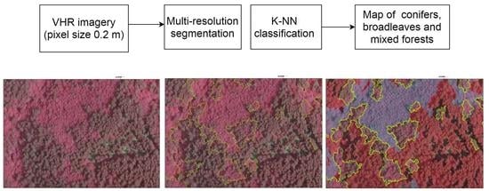
2.3. Methods
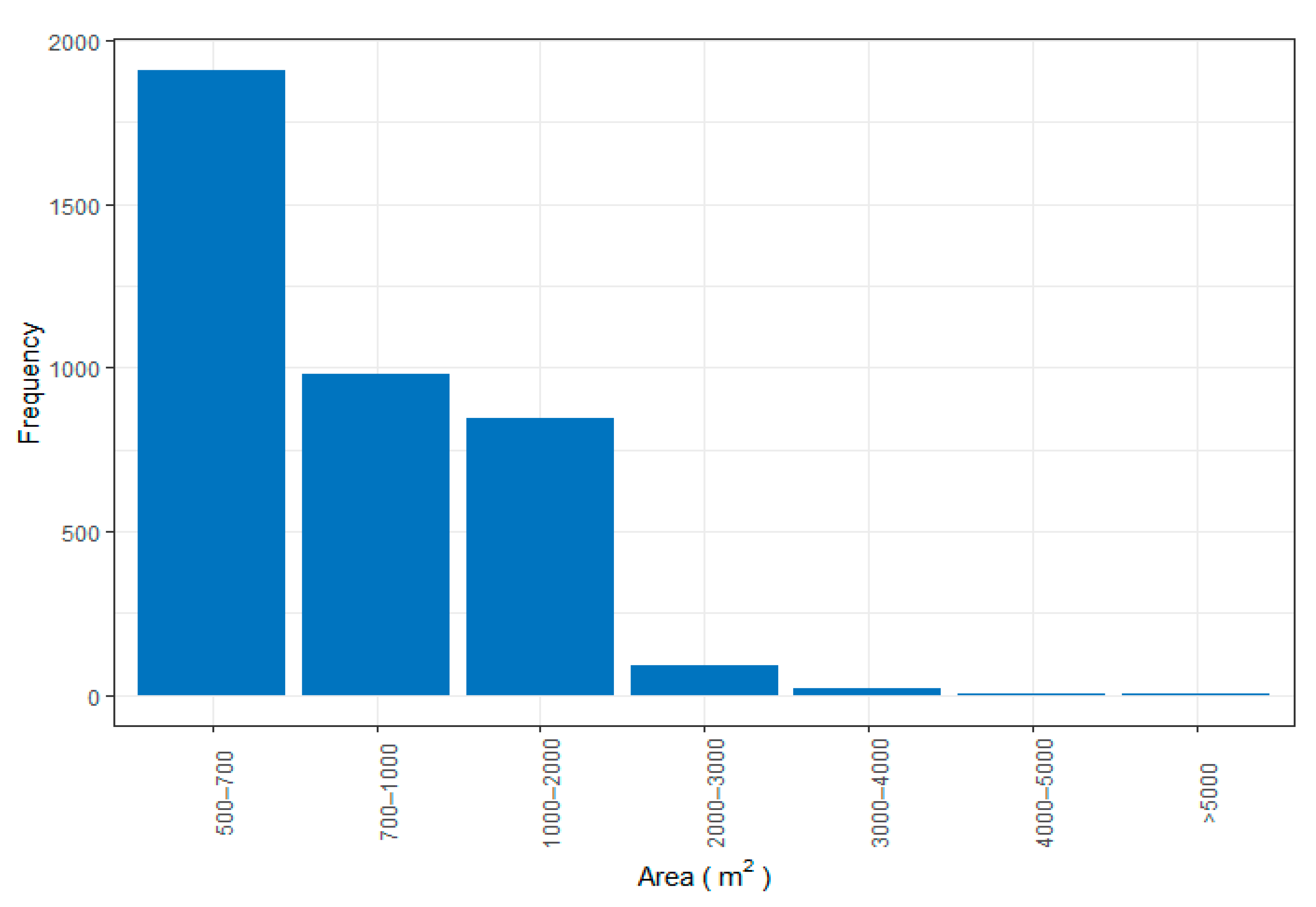
2.3.1. Image Segmentation
2.3.2. Classification of Noise
2.3.3. Training Sample Dataset
2.3.4. Nearest Neighbor Classifier
2.3.5. Mixed Forest Mapping
2.3.6. Validation Dataset
2.3.7. Accuracy Assessment
3. Results
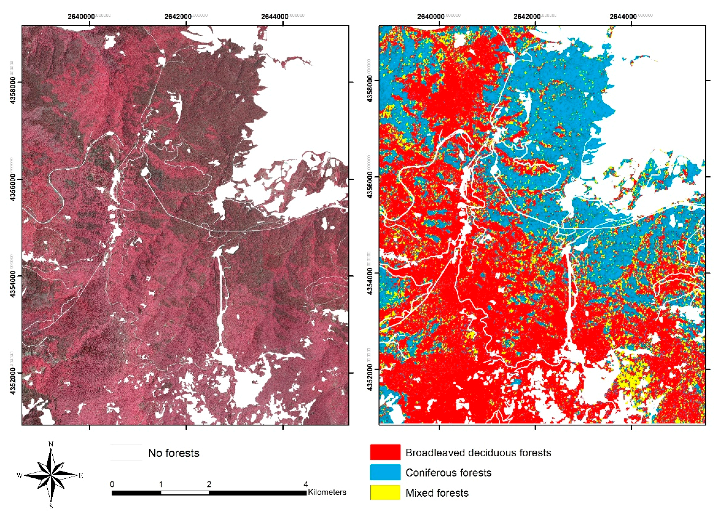
3.1. Forest Types Mapping
3.2. Accuracy Assessment
4. Discussion
5. Conclusions
Author Contributions
Funding
Institutional Review Board Statement
Informed Consent Statement
Acknowledgments
Conflicts of Interest
References
- Bravo-Oviedo, A.; Pretzsch, H.; Ammer, C.; Andenmatten, E.; Barbati, A.; Barreiro, S.; Brang, P.; Bravo, F.; Coll, L.; Corona, P.; et al. European mixed forests: Definition and research perspectives. For. Syst. 2014, 23, 518–533. [Google Scholar] [CrossRef]
- Corine Land Cover Nomenclature Guidelines. Available online: https://land.copernicus.eu/user-corner/technical-library/corine-land-cover-nomenclature-guidelines/html/index-clc-313.html (accessed on 7 May 2019).
- Pardos, M.; del Río, M.; Pretzsch, H.; Jactel, H.; Bielak, K.; Bravo, F.; Brazaitis, G.; Defossez, E.; Engel, M.; Godvod, K.; et al. The greater resilience of mixed forests to drought mainly depends on their composition: Analysis along a climate gradient across Europe. For. Ecol. Manag. 2021, 481, 118687. [Google Scholar] [CrossRef]
- Pretzsch, H.; Steckel, M.; Heym, M.; Biber, P.; Ammer, C.; Ehbrecht, M.; Bielak, K.; Bravo, F.; Ordóñez, C.; Collet, C.; et al. Stand growth and structure of mixed-species and monospecific stands of Scots pine (Pinus sylvestris L.) and oak (Q. robur L., Quercus petraea (Matt.) Liebl.) analysed along a productivity gradient through Europe. Eur. J. For. Res. 2020, 139, 349–367. [Google Scholar] [CrossRef] [Green Version]
- Jonsson, M.; Bengtsson, J.; Gamfeldt, L.; Moen, J.; Snäll, T. Levels of forest ecosystem services depend on specific mixtures of commercial tree species. Nat. Plants 2019, 5, 141–147. [Google Scholar] [CrossRef] [PubMed]
- Jactel, H.; Gritti, E.S.; Drössler, L.; Forrester, D.I.; Mason, W.L.; Morin, X.; Pretzsch, H.; Castagneyrol, B. Positive biodiversity–productivity relationships in forests: Climate matters. Biol. Lett. 2018, 14, 12–15. [Google Scholar] [CrossRef] [PubMed]
- Van Der Plas, F.; Manning, P.; Allan, E.; Scherer-Lorenzen, M.; Verheyen, K.; Wirth, C.; Zavala, M.A.; Hector, A.; Ampoorter, E.; Baeten, L.; et al. Jack-of-all-trades effects drive biodiversity-ecosystem multifunctionality relationships in European forests. Nat. Commun. 2016, 7, 1–11. [Google Scholar] [CrossRef] [PubMed] [Green Version]
- Forrester, D.I.; Bauhus, J. A Review of Processes Behind Diversity—Productivity Relationships in Forests. Curr. For. Rep. 2016, 2, 45–61. [Google Scholar] [CrossRef] [Green Version]
- Tomao, A.; Bonet, J.A.; Martínez de Aragón, J.; De-Miguel, S. Is silviculture able to enhance wild forest mushroom resources? Current knowledge and future perspectives. For. Ecol. Manag. 2017, 402, 102–114. [Google Scholar] [CrossRef] [Green Version]
- Tomao, A.; Antonio Bonet, J.; Castaño, C.; De-Miguel, S. How does forest management affect fungal diversity and community composition? Current knowledge and future perspectives for the conservation of forest fungi. For. Ecol. Manag. 2020, 457, 117678. [Google Scholar] [CrossRef]
- Bauhus, J.; Forrester, D.I.; Pretzsch, H.; Felton, A.; Pyttel, P.; Benneter, A. Silvicultural options for mixed-species stands. In Mixed-Species Forests; Springer: Berlin/Heidelberg, Germany, 2017; pp. 433–501. [Google Scholar]
- Coll, L.; Ameztegui, A.; Collet, C.; Löf, M.; Mason, B.; Pach, M.; Verheyen, K.; Abrudan, I.; Barbati, A.; Barreiro, S.; et al. Knowledge gaps about mixed forests: What do European forest managers want to know and what answers can science provide? For. Ecol. Manag. 2018, 407, 106–115. [Google Scholar] [CrossRef] [Green Version]
- Mustafa, Y.T.; Habeeb, H.N. Object based technique for delineating and mapping 15 tree species using VHR WorldView-2 imagery. Remote Sens. Agric. Ecosyst. Hydrol. XVI 2014, 9239, 92390G. [Google Scholar] [CrossRef]
- Waser, L.T.; Küchler, M.; Jütte, K.; Stampfer, T. Evaluating the potential of worldview-2 data to classify tree species and different levels of ash mortality. Remote Sens. 2014, 6, 4515–4545. [Google Scholar] [CrossRef] [Green Version]
- Madonsela, S.; Cho, M.A.; Mathieu, R.; Mutanga, O.; Ramoelo, A.; Kaszta, Ż.; Van De Kerchove, R.V.; Wolff, E. Multi-phenology WorldView-2 imagery improves remote sensing of savannah tree species. Int. J. Appl. Earth Obs. Geoinf. 2017, 58, 65–73. [Google Scholar] [CrossRef] [Green Version]
- Wu, H.; Levin, N.; Seabrook, L.; Moore, B.D.; McAlpine, C. Mapping foliar nutrition using WorldView-3 and WorldView-2 to assess koala habitat suitability. Remote Sens. 2019, 11, 215. [Google Scholar] [CrossRef] [Green Version]
- Lucas, R.; Rowlands, A.; Brown, A.; Keyworth, S.; Bunting, P. Rule-based classification of multi-temporal satellite imagery for habitat and agricultural land cover mapping. ISPRS J. Photogramm. Remote Sens. 2007, 62, 165–185. [Google Scholar] [CrossRef]
- Lengyel, S.; Déri, E.; Varga, Z.; Horváth, R.; Tóthmérész, B.; Henry, P.Y.; Kobler, A.; Kutnar, L.; Babij, V.; Seliškar, A.; et al. Habitat monitoring in Europe: A description of current practices. Biodivers. Conserv. 2008, 17, 3327–3339. [Google Scholar] [CrossRef]
- Lucas, R.; Medcalf, K.; Brown, A.; Bunting, P.; Breyer, J.; Clewley, D.; Keyworth, S.; Blackmore, P. Updating the Phase 1 habitat map of Wales, UK, using satellite sensor data. ISPRS J. Photogramm. Remote Sens. 2011, 66, 81–102. [Google Scholar] [CrossRef]
- Grabska, E.; Hostert, P.; Pflugmacher, D.; Ostapowicz, K. Forest stand species mapping using the sentinel-2 time series. Remote Sens. 2019, 11, 1197. [Google Scholar] [CrossRef] [Green Version]
- Persson, M.; Lindberg, E.; Reese, H. Tree species classification with multi-temporal Sentinel-2 data. Remote Sens. 2018, 10, 1794. [Google Scholar] [CrossRef] [Green Version]
- Nelson, M. Evaluating Multitemporal Sentinel-2 data for Forest Mapping using Random Forest. Master’s Thesis, Stockholm University, Stockholm, Sweden, 2017. [Google Scholar]
- Immitzer, M.; Vuolo, F.; Atzberger, C. First experience with Sentinel-2 data for crop and tree species classifications in central Europe. Remote Sens. 2016, 8, 166. [Google Scholar] [CrossRef]
- Pu, R.; Landry, S. A comparative analysis of high spatial resolution IKONOS and WorldView-2 imagery for mapping urban tree species. Remote Sens. Environ. 2012, 124, 516–533. [Google Scholar] [CrossRef]
- Pu, R. Broadleaf species recognition with in situ hyperspectral data. Int. J. Remote Sens. 2009, 30, 2759–2779. [Google Scholar] [CrossRef]
- Dalponte, M.; Ørka, H.O.; Gobakken, T.; Gianelle, D.; Næsset, E. Tree species classification in boreal forests with hyperspectral data. IEEE Trans. Geosci. Remote Sens. 2013, 51, 2632–2645. [Google Scholar] [CrossRef]
- Hill, R.A.; Thomson, A.G. Mapping woodland species composition and structure using airborne spectral and LiDAR data. Int. J. Remote Sens. 2005, 26, 3763–3779. [Google Scholar] [CrossRef]
- Dalponte, M.; Bruzzone, L.; Gianelle, D. Tree species classification in the Southern Alps based on the fusion of very high geometrical resolution multispectral/hyperspectral images and LiDAR data. Remote Sens. Environ. 2012, 123, 258–270. [Google Scholar] [CrossRef]
- Blaschke, T.; Hay, G.J.; Kelly, M.; Lang, S.; Hofmann, P.; Addink, E.; Queiroz Feitosa, R.; van der Meer, F.; van der Werff, H.; van Coillie, F.; et al. Geographic Object-Based Image Analysis—Towards a new paradigm. ISPRS J. Photogramm. Remote Sens. 2014. [Google Scholar] [CrossRef] [Green Version]
- Feizizadeh, B.; Kazemi Garajeh, M.; Blaschke, T.; Lakes, T. An object based image analysis applied for volcanic and glacial landforms mapping in Sahand Mountain, Iran. Catena 2021. [Google Scholar] [CrossRef]
- Janowski, L.; Kubacka, M.; Pydyn, A.; Popek, M.; Gajewski, L. From acoustics to underwater archaeology: Deep investigation of a shallow lake using high-resolution hydroacoustics—The case of Lake Lednica, Poland. Archaeometry 2021. [Google Scholar] [CrossRef]
- Rajbhandari, S.; Aryal, J.; Osborn, J.; Lucieer, A.; Musk, R. Leveraging machine learning to extend Ontology-driven Geographic Object-Based Image Analysis (O-GEOBIA): A case study in forest-type mapping. Remote Sens. 2019. [Google Scholar] [CrossRef] [Green Version]
- Uddin, K.; Gilani, H.; Murthy, M.S.R.; Kotru, R.; Qamer, F.M. Forest Condition Monitoring Using Very-High-Resolution Satellite Imagery in a Remote Mountain Watershed in Nepal. Mt. Res. Dev. 2015, 35, 264–277. [Google Scholar] [CrossRef]
- Chehata, N.; Orny, C.; Boukir, S.; Guyon, D.; Wigneron, J.P. Object-based change detection in wind storm-damaged forest using high-resolution multispectral images. Int. J. Remote Sens. 2014, 35, 4758–4777. [Google Scholar] [CrossRef]
- Benz, U.C.; Hofmann, P.; Willhauck, G.; Lingenfelder, I.; Heynen, M. Multi-resolution, object-oriented fuzzy analysis of remote sensing data for GIS-ready information. ISPRS J. Photogramm. Remote Sens. 2004, 58, 239–258. [Google Scholar] [CrossRef]
- Whiteside, T.G.; Boggs, G.S.; Maier, S.W. Comparing object-based and pixel-based classifications for mapping savannas. Int. J. Appl. Earth Obs. Geoinf. 2011, 13, 884–893. [Google Scholar] [CrossRef]
- Laliberte, A.S.; Rango, A.; Havstad, K.M.; Paris, J.F.; Beck, R.F.; McNeely, R.; Gonzalez, A.L. Object-oriented image analysis for mapping shrub encroachment from 1937 to 2003 in southern New Mexico. Remote Sens. Environ. 2004. [Google Scholar] [CrossRef]
- Yu, Q.; Gong, P.; Clinton, N.; Biging, G.; Kelly, M.; Schirokauer, D. Object-based detailed vegetation classification with airborne high spatial resolution remote sensing imagery. Photogramm. Eng. Remote Sens. 2006. [Google Scholar] [CrossRef] [Green Version]
- Bagaram, M.B.; Giuliarelli, D.; Chirici, G.; Giannetti, F.; Barbati, A. UAV remote sensing for biodiversity monitoring: Are forest canopy gaps good covariates? Remote Sens. 2018, 10, 1397. [Google Scholar] [CrossRef]
- Immitzer, M.; Atzberger, C.; Koukal, T. Tree species classification with Random forest using very high spatial resolution 8-band worldView-2 satellite data. Remote Sens. 2012, 4, 2661–2693. [Google Scholar] [CrossRef] [Green Version]
- Geoportale Regione Calabria. Available online: http://www.pcn.minambiente.it/GN/ (accessed on 17 June 2020).
- Brullo, S.; Scelsi, F.; Spampinato, G. Vegetazione dell’Aspromonte; Laruffa: Reggio Calabria, Italy, 2001; ISBN 8872211603. [Google Scholar]
- Terraitaly. Available online: https://www.terraitaly.it/en/ (accessed on 17 June 2020).
- Mather, P.M.; Koch, M. Computer Processing of Remotely-Sensed Images: An Introduction, 4th ed.; Wiley: Hoboken, NJ, USA, 2010; ISBN 9780470742389. [Google Scholar]
- Lyons, M.B.; Keith, D.A.; Phinn, S.R.; Mason, T.J.; Elith, J. A comparison of resampling methods for remote sensing classification and accuracy assessment. Remote Sens. Environ. 2018. [Google Scholar] [CrossRef]
- Alpaydin, E. Design and Analysis of Machine Learning Experiments; MIT Press: Cambridge, MA, USA, 2010. [Google Scholar]
- Thanh Noi, P.; Kappas, M. Comparison of Random Forest, k-Nearest Neighbor, and Support Vector Machine Classifiers for Land Cover Classification Using Sentinel-2 Imagery. Sensors 2017, 18, 18. [Google Scholar] [CrossRef] [Green Version]
- Singh, A.; Halgamuge, M.N.; Lakshmiganthan, R. Impact of Different Data Types on Classifier Performance of Random Forest, Naïve Bayes, and K-Nearest Neighbors Algorithms. Int. J. Adv. Comput. Sci. Appl. 2017, 8, 1–11. [Google Scholar] [CrossRef] [Green Version]
- Oke, O.A.; Thompson, K.A. Distribution models for mountain plant species: The value of elevation. Ecol. Modell. 2015. [Google Scholar] [CrossRef]
- Koukal, T.; Suppan, F.; Schneider, W. The impact of relative radiometric calibration on the accuracy of kNN-predictions of forest attributes. Remote Sens. Environ. 2007. [Google Scholar] [CrossRef]
- Finegold, Y.; Ortmann, A.; Lindquist, E.; d’Annunzio, R.; Sandker, M. Map Accuracy Assessment and Area Estimation: A Practical Guide; Food and Agriculture Organization of the United Nations: Rome, Italy, 2016. [Google Scholar]
- Rosenfield, G.H.; Fitzpatrick-Lins, K. A coefficient of agreement as a measure of thematic classification accuracy. Photogramm. Eng. Remote Sens. 1986, 52, 223–227. [Google Scholar]
- Miraki, M.; Sohrabi, H.; Fatehi, P.; Kneubuehler, M. Individual tree crown delineation from high-resolution UAV images in broadleaf forest. Ecol. Inform. 2021, 61, 101207. [Google Scholar] [CrossRef]
- Schepaschenko, D.; See, L.; Lesiv, M.; Bastin, J.-F.; Mollicone, D.; Tsendbazar, N.-E.; Bastin, L.; McCallum, I.; Bayas, J.C.L.; Baklanov, A. Recent advances in forest observation with visual interpretation of very high-resolution imagery. Surv. Geophys. 2019, 40, 839–862. [Google Scholar] [CrossRef] [Green Version]
- Puletti, N.; Chianucci, F.; Castaldi, C. Use of Sentinel-2 for forest classification in Mediterranean environments. Ann. Silvic. Res 2018, 42, 32–38. [Google Scholar]
- Dechesne, C.; Mallet, C.; Le Bris, A.; Gouet-Brunet, V. Semantic segmentation of forest stands of pure species combining airborne lidar data and very high resolution multispectral imagery. ISPRS J. Photogramm. Remote Sens. 2017, 126, 129–145. [Google Scholar] [CrossRef]
- Hovi, A.; Raitio, P.; Rautiainen, M. A spectral analysis of 25 boreal tree species. Silva Fenn. 2017, 51. [Google Scholar] [CrossRef] [Green Version]
- Drǎguţ, L.; Csillik, O.; Eisank, C.; Tiede, D. Automated parameterisation for multi-scale image segmentation on multiple layers. ISPRS J. Photogramm. Remote Sens. 2014. [Google Scholar] [CrossRef] [Green Version]


| Classes | Parameter | Threshold |
|---|---|---|
| Dark Shade | Mean green | ≤35 |
| Light Shade | Mean green | >35 & ≤45 |
| Grassland | Brightness | ≥110 |
| Max diff | ≥0.08 ≤0.329 |
| Classification Code | Tree Crown Assemblage | Number of Samples |
|---|---|---|
| 0 | Broadleaved deciduous forest | 76 |
| 1 | Coniferous forest | 39 |
| Total | 115 |
| Code | Class | Description |
|---|---|---|
| 0 | Broadleaved deciduous forest | No less than 70% of the total area of the coarser polygons (FS150) is covered by sub-polygons (FS80) classified as broadleaved deciduous forest |
| 1 | Coniferous forest | No less than 70% of the total area of the coarser polygons (FS150) is covered by sub-polygons (FS80) classified as coniferous forest |
| 2 | Mixed forest of broadleaved deciduous and coniferous trees | Both FS80 polygons classified as broadleaves and FS80 polygons classified as conifers occupy at least 30%, but maximum 70%, of the total area of coarser polygons (FS150) |
| Code | Class | Number of Polygons for Map Validation | Surface (ha) | % |
|---|---|---|---|---|
| 0 | Broadleaved deciduous forest | 47 | 69.01 | 50 |
| 1 | Coniferous forest | 34 | 35.41 | 25 |
| 2 | Mixed forest of broadleaved deciduous and coniferous trees | 33 | 33.31 | 24 |
| tot | 114 | 137.73 | 100 |
| Code | Classes | Area (ha) | %Area |
|---|---|---|---|
| 0 | Broadleaved deciduous forest | 2502.44 | 55 |
| 1 | Coniferous forest | 1553.44 | 34 |
| 2 | Mixed forest of broadleaved deciduous and coniferous trees | 497.1 | 11 |
| Total | 4552.98 | 100 |
| 0 | 1 | 2 | |
|---|---|---|---|
| UA | 0.93 | 0.90 | 0.73 |
| PA | 0.85 | 0.88 | 0.84 |
| OA | 0.85 | ||
| K | 0.78 |
Publisher’s Note: MDPI stays neutral with regard to jurisdictional claims in published maps and institutional affiliations. |
© 2021 by the authors. Licensee MDPI, Basel, Switzerland. This article is an open access article distributed under the terms and conditions of the Creative Commons Attribution (CC BY) license (https://creativecommons.org/licenses/by/4.0/).
Share and Cite
Oreti, L.; Giuliarelli, D.; Tomao, A.; Barbati, A. Object Oriented Classification for Mapping Mixed and Pure Forest Stands Using Very-High Resolution Imagery. Remote Sens. 2021, 13, 2508. https://doi.org/10.3390/rs13132508
Oreti L, Giuliarelli D, Tomao A, Barbati A. Object Oriented Classification for Mapping Mixed and Pure Forest Stands Using Very-High Resolution Imagery. Remote Sensing. 2021; 13(13):2508. https://doi.org/10.3390/rs13132508
Chicago/Turabian StyleOreti, Loredana, Diego Giuliarelli, Antonio Tomao, and Anna Barbati. 2021. "Object Oriented Classification for Mapping Mixed and Pure Forest Stands Using Very-High Resolution Imagery" Remote Sensing 13, no. 13: 2508. https://doi.org/10.3390/rs13132508
APA StyleOreti, L., Giuliarelli, D., Tomao, A., & Barbati, A. (2021). Object Oriented Classification for Mapping Mixed and Pure Forest Stands Using Very-High Resolution Imagery. Remote Sensing, 13(13), 2508. https://doi.org/10.3390/rs13132508