Article

Parts-per-Object Count in Agricultural Images: Solving Phenotyping Problems via a Single Deep Neural Network

by
Faina Khoroshevsky
*,
Stanislav Khoroshevsky
and
Aharon Bar-Hillel
Department of Industrial Engineering and Management, Faculty of Engineering Sciences, Ben-Gurion University of the Negev, Beer-Sheva P.O. Box 653, Israel
*
Author to whom correspondence should be addressed.
Remote Sens. 2021, 13(13), 2496; https://doi.org/10.3390/rs13132496
Submission received: 10 March 2021 / Revised: 7 June 2021 / Accepted: 16 June 2021 / Published: 26 June 2021

Abstract

:
Solving many phenotyping problems involves not only automatic detection of objects in an image, but also counting the number of parts per object. We propose a solution in the form of a single deep network, tested for three agricultural datasets pertaining to bananas-per-bunch, spikelets-per-wheat-spike, and berries-per-grape-cluster. The suggested network incorporates object detection, object resizing, and part counting as modules in a single deep network, with several variants tested. The detection module is based on a Retina-Net architecture, whereas for the counting modules, two different architectures are examined: the first based on direct regression of the predicted count, and the other on explicit parts detection and counting. The results are promising, with the mean relative deviation between estimated and visible part count in the range of 9.2% to 11.5%. Further inference of count-based yield related statistics is considered. For banana bunches, the actual banana count (including occluded bananas) is inferred from the count of visible bananas. For spikelets-per-wheat-spike, robust estimation methods are employed to get the average spikelet count across the field, which is an effective yield estimator.

Graphical Abstract

1. Introduction

This work handles a specific family of phenotyping problems: visual object’s part counting, done by first detecting the objects in the image, and then counting their constituting parts. Such problems repeatedly arise in field phenotyping contexts. Examples include counting the number of bananas in banana bunches [1], spikelets in wheat spikes [2,3], berries per grape cluster [4], flowers on apple trees [5,6], leaves in potted plants [7,8], or mangoes per-tree [9]. Specifically, in this work we address the first three above-mentioned problems. Image examples with annotations for each task are shown in Figure 1.
Agricultural applications often incorporate robotic systems to reduce labor tensions, especially in developing countries [10,11]. Such systems, as well as systematic yield estimation, require reliable computer vision methods operating in field conditions [11,12,13]. This environment is highly challenging: crops vary significantly in shape, size, and color, and there are significant illumination variance and occlusion problems [11]. The part counting task addressed here has to be solved robustly in this complex environment.
In many cases, part count is an important yield indicator, and measuring it automatically is important for yield prediction and breed selection [4,9,14,15]. Specifically, spikelets counting provides yield quantification for wheat crop and thus can assist in crop management [3]. The number of bananas in a bunch is related to bunch weight and thus productivity [16]. For grapes, yield estimation of a vineyard can be performed using berry detection [4,17] and counting [15]. These three very different problems are handled here with the same algorithm, thus demonstrating that the proposed method is fairly general and can handle different part-counting problems with minor adjustments. While such problems usually involve (object) detection and (part) counting, they should not be confused with single-stage counting or detection problems, and require a non-trivial combination of them, as presented in this work.
Object detection is a first step in several types of agricultural applications including robotic harvesting and spraying [15,18,19], measurement of object properties [20,21,22,23], or object (not parts) counting [24]. Object count is a common phenotype needed for tasks as yield estimation [4,24,25,26], blossom level estimation for fruit thinning decisions [5,6,27], or plant’s leaf counting for growth stage and health estimation [7,8,28,29].
The two tasks of detection and counting were approached with both traditional computer vision techniques and deep Convolutional Neural Networks (CNNs). Specifically, fruit detection systems using traditional techniques were presented in [10,13], and CNN-based works can be found in [30,31]. One line of influential detection networks includes two-stage networks like Faster R-CNN [32] or Mask R-CNN [33]. Another line of work includes fully differentiable one-stage architectures. Early one-stage networks as YOLO [34] and SSD [35] presented faster detectors, but with accuracy lower by 10–40% relative to two-stage methods [36]. Later, one-stage networks like RetinaNet [36] and more recently EfficientDet [37] were able to close the accuracy gap. An advanced version of YOLO, the YOLOv3 model [38], was successfully augmented and applied recently for tomato [30] and kiwi fruit [31] detection.
For counting, a successful work based on traditional techniques can be found in [39,40,41], but CNNs designed for the task currently provide the state-of-the-art accuracy [42,43].
In general, deep learning methods can produce higher accuracy, but often require a large annotated image sample and a long training schedule [11]. On the other hand, CNNs avoid the tedious feature engineering process and are often able to provide general solutions applicable to a family of different but related tasks.
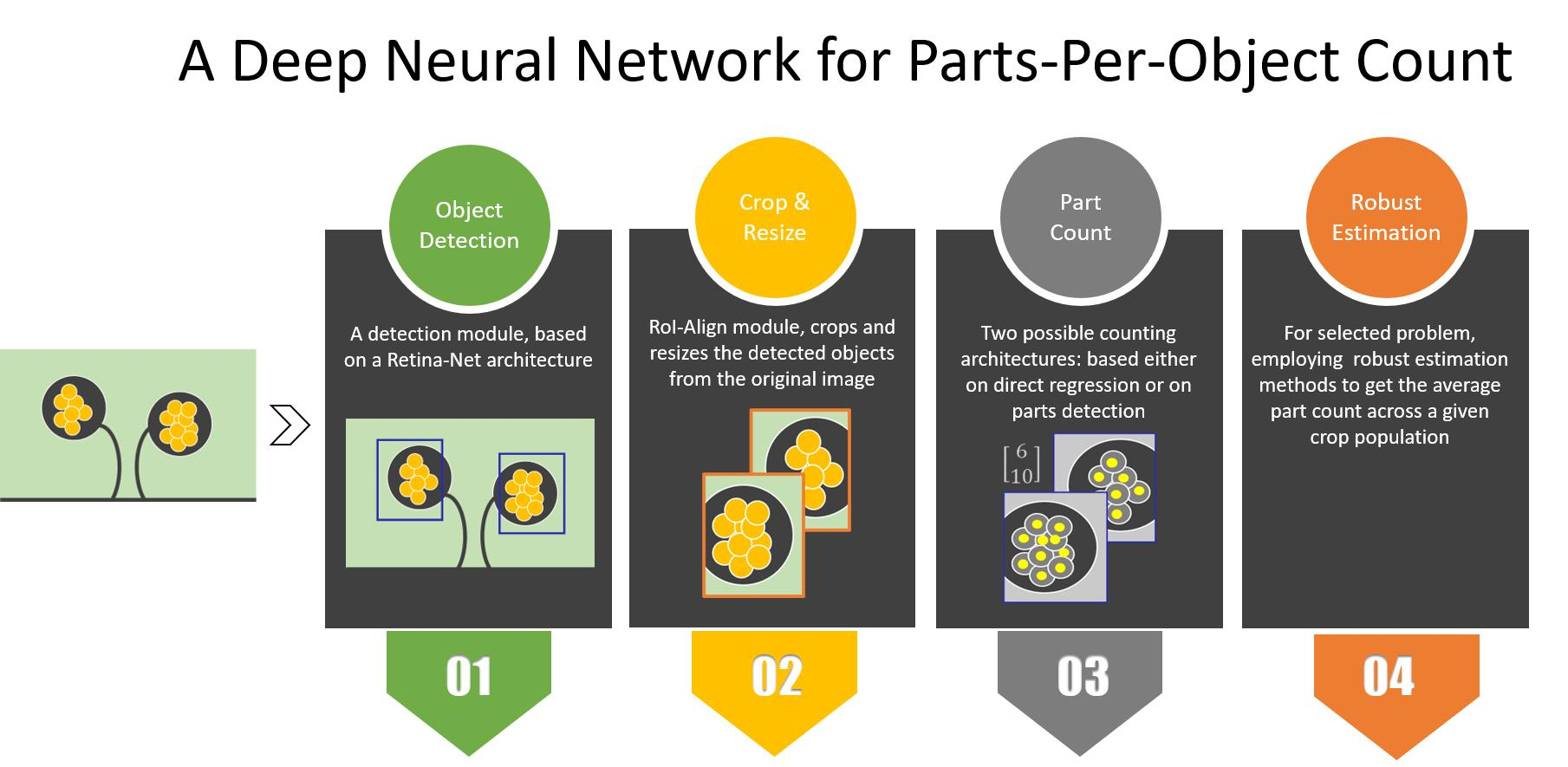
The approach suggested in this work handles the object part counting with a two-stage approach of (a) detecting the objects and (b) counting the parts in their detected regions. However, the combination of these two stages into a single system raises several questions. First, parts are much smaller than their containing objects, so scale difference should be accounted for. A second set of considerations arises w.r.t the combination of object detection and part counting into a single network. Should the two modules share components (like a shared backbone subnetwork)? Should they be trained together, end-to-end, or independently? How should the detection confidence threshold, above which objects are sent for counting, be determined? In this work, we explore the design space of possible solutions for part-counting networks and find a good solution based on a single network combining stages for a detector, scaling, and counting.
One may wonder why the “parts counting” task (which is essentially a “detect-then-count” procedure) cannot be reduced into plain counting, by simply taking pictures containing a single object in each image. Indeed, in principal this is possible. In some agricultural contexts, the two-stage part-object nature was bypassed by using images of a single centralized object [6,28,29]. However, solving a part counting problem by taking images of single objects has significant disadvantages. The counting procedure needs to be automated, rather than being done by a tedious manual approach. If a human has to detect the objects and take single-object images, the process is partially manual. Therefore, it is slower, costs more, and is less scalable than a fully automated system. Another option is to have a robotic system first detecting the objects, than moving to a close position to each object for taking a second image, isolating it from a wider scene. While this does not involve human intervention, such a system is much more complex to develop, and it also is likely to be slower than a system based on high resolution images containing multiple objects. Therefore, for automatic and flexible field phenotyping, the solution of keeping one object per image is significantly less scalable.
As we are interested in designing a unified network for the part counting task, we rely on a one-stage architecture as a baseline detector in this work. Specifically, we chose RetinaNet that introduced the use of a Feature Pyramid Network (FPN) [44] for handling larger scale variability of objects and a “focal loss” variant which balances between positive examples (which are few in a detection task) and negative examples.
As for the counting section, one influential approach for CNN-based counting is based on explicit object localization: objects are first detected, then counted. The detection task can be defined as detection of the object’s centers, and so the output is a density map showing where objecthood probability is high [8,45]. In [2], spike and spikelets were counted independently with a density estimation approach, providing very good results of relative error <1% for spikelets and <5% for spikes. However, data were obtained in glassdoor conditions. In [46], it was shown that density map estimation can stay reliable through significant input domain shift when proper techniques of domain-adversarial learning are used. Alternatively, localization can be based on bounding box detection [14,24,47] or segmentation [48,49,50]. These methods require object location annotations like center point annotations (for density estimation), bounding boxes (for detection), or surrounding polygons (for segmentation). The second successful approach is via a global [7,8,51] or local direct regression model [26,52]. In global regression, the model implements a function mapping the entire image (or region) to a single number, which is the predicted count. In local regression the image (or region) is divided into local regions and each of them is mapped to a local predicted count. The local counts are then summed to get the global count.
The literature contains contrasting evidence regarding the relative accuracy of localization-based versus direct regression methods, and the better choice seems to depend on data distribution and quantity, and on availability of annotation. In [47], a detection based method was found superior to direct regression and it is claimed to be more robust to train–test domain changes. By contrast, in [52] direct regression provides higher accuracy than density estimation. In [8], the two approaches show similar performance. An advantage of detection based methods is in being more “explainable”, as it allows to visually inspect where in the image the network finds objects. However, more computation effort is required at test time, and an additional annotating effort at train time. In this work, we experiment with both localization-based and direct regression approaches in the counting section of the network.
While the network proposed is counting the number of visible object parts, the real quantity of interest is the actual part count, which includes also occluded parts. This gap is more pronounced for round objects like a banana bunch, and less for flatter objects like spikes. Following the work in [53], this problem can be overcome by assuming that on average there is a constant ratio of visible to occluded fruits, and training a linear regressor for inferring the actual count from the visible count. We show in our banana experiments that this technique is indeed applicable to part counting, with minor loss in accuracy.
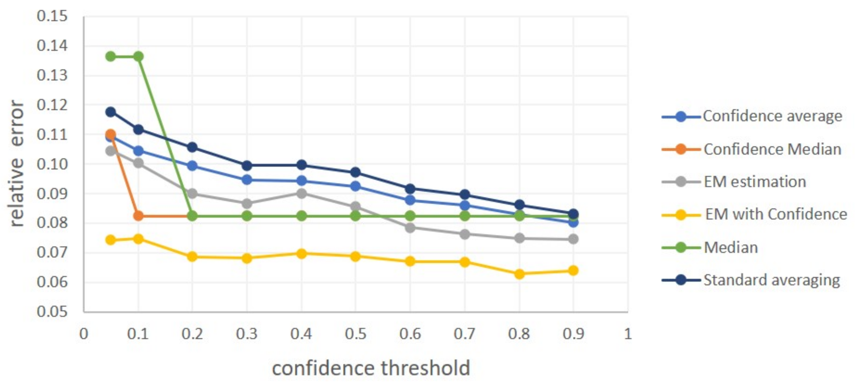
Beyond part counting for a specific object, in yield estimation we are often interested in the average count across an object population. This is the case for example with spikelet count, where the average count over an entire plot or field are of interest. While the solution can be obtained trivially by plain averaging, other options are possible. First, a solution can be obtained by independent plain counting of objects and parts, then dividing the numbers. Second, when a two-stage approach is used, plain averaging includes in the average “false counts” generated by false detections of non-objects. To reduce the impact of false counts, robust estimation methods can be used. We experiment in the space of possible solutions and find that a combination of lower detection thresholds and robust estimation, based on Gaussian assumptions, provides the best alternative.
Our contribution is therefore as follows:
  • Exploring the design space possible for part counting networks with respect to architecture, training methodology and component reuse, and finding a successful general part counting algorithm.
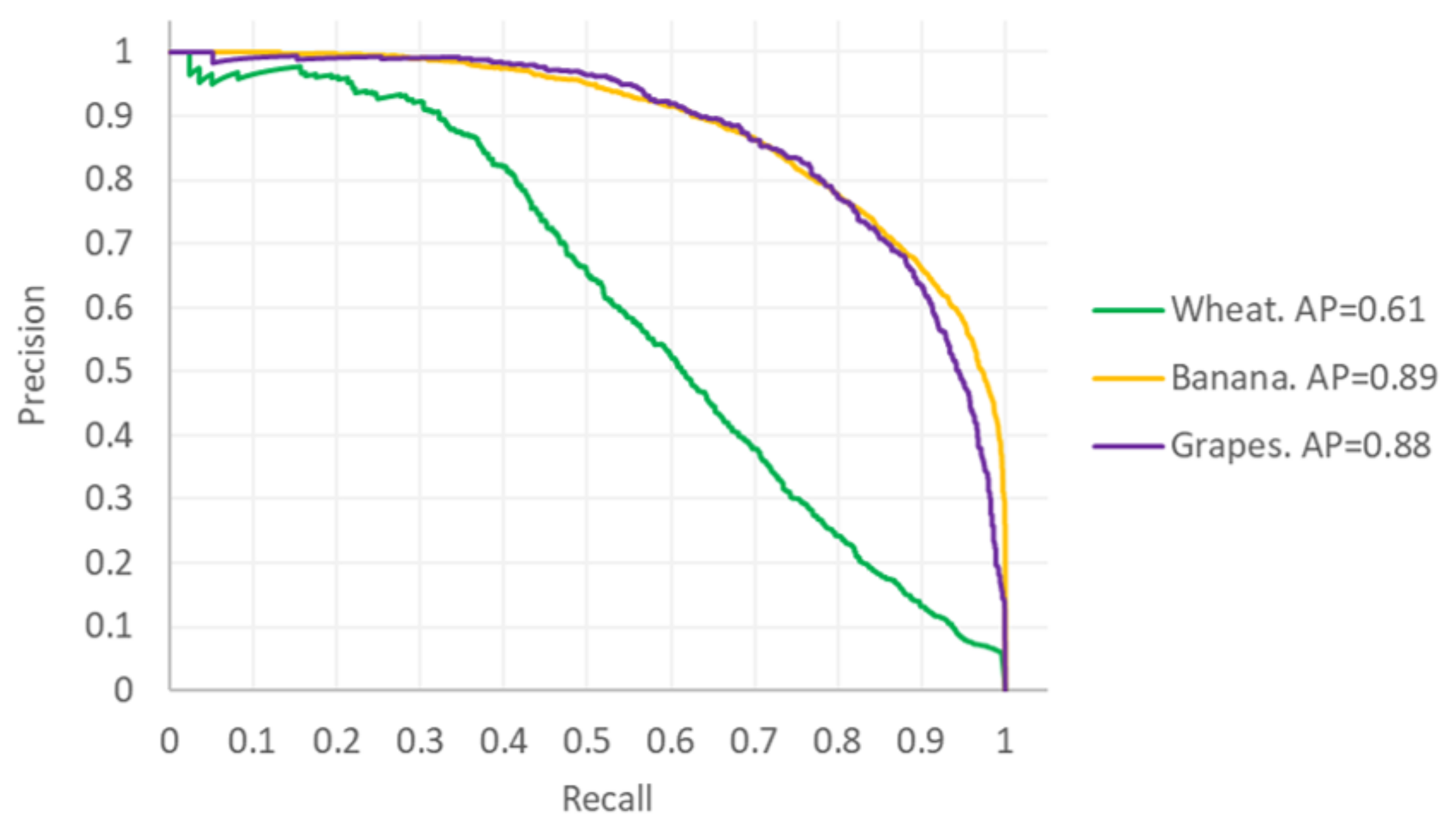
  • Showing the applicability of the developed method to three important phenotyping problems, with low count deviation of 9.2–11.5%.
  • Developing a robust estimation module enabling better estimation of population average part count (compared to plain averaging) and showing its utility for wheat spikelet count.
An earlier version of this paper was published as a conference paper [54]. The current paper, however, contains significant added content. First, we experiment with the architecture of the suggested network in [54]. It includes two independent sections for detection and counting, where each has its own copy of ResNet-50-based [55] backbone module. Two alternative architectures reducing this redundancy were considered. One is based on using a single backbone module with shared weights in both sections of the network. In the other, the backbone module is dropped from the counting section and replaced by a cropped and resized representation of the detected object, obtained by the detector’s backbone. A set of systematic experiments were carried in order to check component reuse opportunities and training methodology, revealing a possible trade-off between accuracy, model size, and computational complexity. Second, the method was tested on a new dataset not included in the conference version, the grapes dataset, which is based on the publicly available Embrapa WGISD212 dataset [15,56]. Third, the new task of average spikelet-per-spike count per field, is considered here. As plain averaging of the sample would produce a biased estimator of this value, due to false alarms, an alternative approach is presented. It is based on applying the robust mean estimation methods on top of the network’s estimates of the spikelets-per-spike values. These methods, presented here for the first time, were tested using new images, obtained from six different field plots.
The rest of the paper is organized as follows: we describe the data and the algorithm in Section 2, present results in Section 3, discussion in Section 4 and conclusions in Section 5.

2. Materials and Methods

We describe the used datasets in Section 2.1, the networks’ architecture in Section 2.2, robust mean estimation methods in Section 2.3, the training procedure in Section 2.4, and performance evaluation methodology in Section 2.5.

2.1. The Datasets

This work is tested on three image datasets collected in field conditions. All images were annotated with bounding boxes for countable objects, and with center dot annotations for each part of an annotated object. Countable objects were defined as “objects for which a human annotator can visually count the parts”. This entails that the object should not be partially occluded or blurred. The banana and wheat data were obtained by the Israel Phenomics Consortium and the grape data [15,56] are publicly available. The number of images, objects, and parts used for training, validation, and testing is listed in Table 1. Additional data of banana and wheat were collected for the estimation of actual physical count of bananas-per-bunch and mean count of spikelets-per-spike of different wheat fields. This additional data are discussed in Section 2.1.2 and Section 2.1.3, respectively.

2.1.1. Datasets for Parts-per-Object Count Estimation

Wheat dataset: The collected dataset includes 101 RGB images taken in an agricultural facility in the Central District of Israel. High-resolution, 6000 × 4000 , images of several wheat varieties in field conditions were taken using a commercial DSLR camera. As the original images included hundreds of wheat spikes, several regions (usually 4–5, 1020 × 830 crops) in focus were handpicked in each image. These areas were cropped and treated as separate images that were passed for annotation of well defined, measurable spikes.
Bananas dataset: 141 RGB images were captured in a facility in the Northern District of Israel. Images included banana bunches of different varieties and stages of the reproductive phase. These were taken using a commercial 9 MP–12 MP mobile device cameras and a digital point-and-shoot cameras in field conditions. The common resolutions were 2340 × 4160 and 3024 × 4032 .
Grapes dataset: This data are based on the publicly available Embrapa WGISD dataset, presented in [15,56]. As our task is to detect only countable objects, we used only 111 out of the available 300 images that contained such objects. The provided bounding box annotations of fully visible and countable grape clusters were kept, and dot annotations of the berries for those countable clusters were added. The dot annotations were made publicly available as part of Embrapa WGISD dataset extension.

2.1.2. Data for Physical Counting of Bananas-per-Bunch

An additional dataset was collected to investigate the relation between actual and visual banana count, containing 91 images of 31 banana bunches (objects) with known actual count, photographed from 2–3 viewpoints each. The total number of visible banana fruits (parts) was 7284.

2.1.3. Data for Entire Wheat Field Robust Estimation

In order to test estimation methods (Section 2.3) for the field-average spikelets-per-spike count, additional images from several fields were obtained. These images were annotated similarly to the original wheat data described in Section 2.1.1. In total, these data consist of six different field plots, and the annotations of data per field plot is presented at Table 2. A validation set was created by sampling 40 % of the images of “Plot 1” (the plot with the largest annotation data) in order to choose the hyper parameters for the robust estimation methods (as presented at Section 3.3).

2.2. Networks’ Architecture

The suggested network is comprised of several components. First is a detection section responsible for detecting the objects of interest. These are passed to an RoI-Align module [33] that crops and resizes the detected objects from the original image. The crops are passed to a counting section, in which each crop is treated as an independent input image. It is assumed that each crop contains a single detected object, and the counting section outputs the parts count for that object. The assumption’s correctness naturally depends on the performance of the object detection section. The basic composition of the detection and counting network is demonstrated in Figure 2.
The detection section is a re-implementation of the RetinaNet architecture, composed of “Backbone”, “Find”, and “Where” modules, whose details are explained in Section 2.2.1. The RoI-Align module receives as input the original image and a set of rectangle coordinates of n d detected objects. By re-sampling the image according to the given coordinates, it outputs a tensor of size s × s × n d of image crops, where s is the new object size (empirically set to 640). Such resizing allows handling the significant variation in object size of the different datasets without a need for data-specific configuration.
The counting section includes re-implementations of the two counters proposed in [8], composed using “Backbone”, “Find”, and “Count” modules. We have experimented with two different counters, one based on direct regression (Multiple Scale Regression-MSR) and the other on explicit part detection (Detection+Regression-D+R). A specific network contains either the MSR or the D+R counter, but not both. Modules re-used in different sections (“Backbone” and “Find” appear in both the detector and counter sections) share code and architecture, but not parameters. The counters and their composition using the modules are described in Section 2.2.2.

2.2.1. Detection Architecture

The relevant modules for the detection section of the network are the following:
“Backbone”: A module used for creating a dense feature-rich representation of the image. It is based on applying ResNet-50 [55] as a dense convolutional network followed by an FPN on top of it. The FPN architecture generates a rich 5-scale feature pyramid representation of the input image, with the output tensors termed P 3 P 7 . These tensors include similar representations of the original image in multiple octaves, with P i twice smaller than P i 1 in its spatial dimensions and has 256 maps each. Therefore, they enable object detection at multiple scales. In all experiments, we have used the ResNet-50 network with weights pretrained on ImageNet and fine-tuned them.
“Find” (for detection): The module includes 4 convolutional layers { g i } i = 1 4 , with 256 filters each, culminating in an output map F by a fifth convolutional layer. It is trained for spatially locating objects in an input tensor representation. Different output modes are supported for the detection and count sections.
For the detection pipeline, it implements the fully convolutional classification subnetwork of RetinaNet, predicting the object presence probability at each spatial position of the input tensor. At each position, this probability is estimated for nine anchor rectangles of predefined sizes and aspect ratios. The output tensor F is thus with the same spatial dimensions as the input, but with nine score maps. The “Find” module processes independently all the five pyramid tensors produced by the Backbone’s FPN, thus it produces 5 output tensors. It is trained with the Focal Loss, designed to address imbalance between foreground and background classes during training [36].
“Where”: Like the “Find” module, this module processes all the pyramid tensors P 3 P 7 , and produces 5 output tensors, by implementing the bounding box regression subnetwork of RetinaNet. For each input tensor, it predicts for every position and possible anchor (among the nine considered), a 4-dimensional bounding box refinement vector. The vector includes corrections required for the bounding box to better match the object in its ( x , y , w i d t h , h e i g h t ) parameters. Inference is done by applying, on each of the inputs, 5 convolutional layers, where each keeps the same spatial dimensions as the input pyramid tensor. The first 4 layers have 256 filters each, and the fifth has 4 filters (so the output includes 36 maps overall). It is trained by propagating a smooth- L 1 -regression loss matching the predicted values to ground-truth rectangles—only for anchors with relevant objects.
“Get final bounding boxes”: This function accepts the output tensors of the “Find” and “Where” modules and creates a refined list of predicted boxes containing presumed objects. It filters boxes with predicted object probability higher than a threshold from the “Find” module, and decodes the refined boxes for them according to the “Where” module. A threshold of 0.7 is used as default, but it is tuned to maximize accuracy in certain contexts (see Section 3.3.2). The predictions from all pyramid levels are merged, and a non-maximum suppression procedure with a threshold of 0.3 is applied to yield the final detections list.

2.2.2. Counting Architecture

Given an input image with a single object, the counting section outputs the count value of its parts. Following the work in [8], we experimented with the implementation of the MSR algorithm for direct regression, and a re-implementation of the D+R algorithm, which predicts a heat map of part center locations in addition to counting them. In both cases, the counting section starts with a second “Backbone” module receiving as input detected object regions after resize from the ROI-align module.
MSR “Count”: In this module, the representation tensors P 3 P 7 generated by the “Backbone”, or a subset of them, are each sent to a direct regression module, so multiple count estimations are produced based on different resolutions. This regression module includes two 3 × 3 convolutional layers with 256 output maps, where each keeps the same spatial dimensions of its input, followed by Global Average Pooling (GAP), flattening the maps to a 256 × 1 representation which is fed into two fully connected layers in decreasing sizes, 128 and 64, respectively. It outputs two neurons: the first predicts the expected count, and the second estimates the variance of the error expected in prediction, using the loss function suggested in [57]. Among the five count estimates made based on the considered resolutions, the one with the lowest predicted variance for the input image is chosen.
For the D+R variation, the count section includes a “Find” module variation described next, and then a different “Count” module.
“Find” (for counting): This module has similar architecture to the “Find” module used in detection, but it is used to find center points instead of bounding box rectangles. The module operates only on the high-resolution pyramid scale ( P 3 ), and a single output map of the same resolution is created, stating the probability of part presence at each location. To learn this network, a ground truth heat map is created in training, with a Gaussian kernel placed around each part’s center. Like in the detection “Find” module, four convolutional layers are used, but then a single final map is predicted as output by using a fifth convolutional layer with one filter. It is trained to mimic the ground truth heat map using a dense L 1 regression loss.
Following the work in [8], we tested the option of guiding internal layers by predicting an intermediate heat map after each convolutional layer, and forcing it to mimic the ground truth heat map with additional regression losses. When this is done, the intermediate guiding heat maps are created with decreasing kernel size, so the heat map regression task is cruder and simpler at initial layers.
D+R “Count”: This module gets from the “Find” module the predicted heat map and the feature tensor g 4 preceding it, and provides a count estimate based on them. It is an implementation of the “Counting subnetwork” of the D+R pipeline of [8]. The heat map is subjected to a smooth non-maxima suppression operation, keeping activity of the most active points close to ones while all others are zeroed. The remaining active points are object center predictions, and a global sum operation gives an initial detection-based estimator of the count. In addition to this path, the tensor preceding the map is globally summed to extract additional useful features, and the final count estimate is computed as linear regression from these features and the detection-based estimate.

2.3. Average Count Estimation

For estimation of average part count, a possible approach may avoid part counting of specific objects altogether. Such approach is discussed in Section 2.3.1. Another alternative is to use an estimator of part-count-per-object, as the suggested network, but apply robust mean estimation methods to its outputs. Such methods are discussed in Section 2.3.2.

2.3.1. Estimation with Global Counts

An alternative approach for obtaining the average of parts-per-object in a set of images is as follows: (1) detect all the objects in the images and count them, (2) independently detect all the parts and count them, and (3) divide the two counts to get the average of interest. In this approach, mean parts-per-object estimation is reduced to plain detection and can be carried with standard detection networks.
While simple, this approach suffers from several disadvantages compared to the two staged approach. First, it does not include a resize mechanism enlarging the relevant objects, thus detection of the small parts is more difficult and less reliable. In addition, when parts are searched for in the entire image, and not only in the object bounding boxes, part false alarms are more likely. Second, not all objects are “countable”, due to problems of scale, blur or partial occlusion. For example, in many spikes only part of the spikelets can be observed. Independent counting of parts is therefore likely to include parts which do not belong to countable objects. If the detector is detecting only “countable” objects, the division will produce an overestimation of the mean count. We test the independent count idea empirically in Section 3.3.1.

2.3.2. Robust Mean Estimation

Assume a population of N object detections was used to produce a sample of S = { c i } i = 1 N part count estimates. Our task is to estimate the mean part count across true objects, but the sample S contains a mixture of valid counts, emerging from correct object detections, and irrelevant pseudo counts, created by false detections. False detections often emerge from partially occluded or mislocalized objects, and tend to produce lower part count estimates. Plain averaging of the sample would hence produce a biased estimator of the part count mean. The severity of the false counts problem can be reduced by using a high threshold t over the detection confidence value, thus reducing the number of false detections. However, the utility of this approach is limited: it reduces the sample size used for mean estimation, and false detections, though in lower quantities, still remain.
While full separation between false and true detections is not possible, there are clues softly differentiating between true and false counts, which may enable better mean estimation. One such clue is the difference between count estimate distributions, with false counts having a lower mean. A second clue is a difference in their detection confidence score distribution. These values are provided by the detection module. For false object detections, they often have lower values. We next present several alternatives for obtaining robust mean estimators based on these clues.
Expectation Maximization (EM) for a mixture of Gaussians: We may assume that the sample S arises from a mixture of two Gaussians. True counts arise from a Gaussian distribution G ( c | μ 1 , σ 1 ) = 1 2 π σ 1 exp ( ( c μ 1 ) 2 σ 1 2 ) , and false counts from a second Gaussian G ( c | μ 2 , σ 2 ). The probability of a count value c is thus given by
P ( c θ ) = α · G ( c μ 1 , σ 1 ) + ( 1 α ) · G ( c μ 2 , σ 2 )
where α is the probability of correct detection (the probability of a detection to reflect a real countable object), and θ = { μ 1 , σ 1 , μ 2 , σ 2 , α } are the model parameters. The parameters θ can be estimated by finding a maximum likelihood solution
θ * = a r g m a x θ log P ( S | θ ) = a r g m a x θ i = 1 N log P ( c i | θ )
As there is no closed form solution for this optimization problem, a popular strategy is to estimate θ using an EM procedure. In this procedure, additional hidden binary variables { h i } i = 1 N are introduced. If h i = 1 , sample i is assumed to belong to a correctly detected object, and if h i = 2 , it belongs to a false detection. The parameter α is this framework is interpreted as the prior probability α = p ( h = 1 ) , and we set it to 0.5 in our experiments with this method. The EM procedure iterates between estimating w i j = p ( h i = j | c i , θ ) (that’s an Expectation step), and re-estimation of θ using the sample weights { w i j } i = 1 , j = 1 N , 2 (a Maximization step). The procedure is guarantied to converge to a local maximum of the sample likelihood. Once θ has converged, m a x ( μ 1 , μ 2 ) can be used as the count mean estimation, as we assume the average of true counts is larger than the average of false counts.
Weighted average with detection confidence scores: Assume now that the sample is of the form { ( c i , s i ) } i = 1 N , i.e., each count c i has an associated confidence value s i from the detection network module. A simple option for obtaining a mean estimator with more weight on confident detections is the weighted average
i = 1 N s i · c i i = 1 N c i
Median-based scores: A common approach for reducing the exposure of mean estimation to outlier measurements is using the median instead of the average as a mean estimator. For a simple Gaussian or otherwise symmetric distribution the median provides an unbiased mean estimator, and it is significantly less vulnerable to the existence of false measurements. The median idea can be simply extended to a confidence weighted sample. In this generalization samples are sorted in ascending measurement (count) values, and their confidence weights are normalized by defining s i = s i / j = 1 N s j so i = 1 N s i = 1 . The confidence-weighted median is the sample c i for which u ( i ) = j = 1 i s ( i ) = 0.5 if such an element exist. If not, the first element c i for which u i > 0.5 is found and the median is computed as a confidence weighted average between this element and its predecessor
s j 1 · c j 1 + s j · c j s j 1 + s j
Combining EM with confidence scores: The count distribution differences and the confidence value are two different, and possibly complementary, sources of information for mean estimation. We can combine them in the probabilistic EM-procedure if we assume that the probability α i = p ( h i = 1 ) of sample i to be a valid object detection is given by the confidence value s i . The EM algorithm can be easily extended to accept such sample-dependent { α i } i = 1 N values as input instead of estimating a global parameter α . The full EM procedure accepting example confidence values { α i } i = 1 N is presented in Algorithm 1.
Algorithm 1: Gaussian mixture EM with sample confidence values.
Remotesensing 13 02496 i001
Softening of the confidence scores: The detection probability estimate provided by the “find” module is often too confident (close to 1 or 0), in a manner that damages the confidence-based methods suggested above. We suggest to calibrate it toward a “softer” estimate as follows. For each candidate bounding box, the objecthood probability confidence estimate s [ 0 , 1 ] is derived from an output neuron of the network l R (the “logit”) by a sigmoid functions, i.e.,
s = σ ( l ) = 1 1 + e x p ( l ) , l = σ 1 ( s ) = log 1 s s
The logit l has positive values for bounding boxes with high objecthood probability and negative values for boxes with low probability. The soften confidence probability is introduced by multiplying the logit l with a constant β ( 0 , 1 ) which makes it less extreme. Explicitly the soften probability estimate s β is obtained as a function of s by
s β ( s ) = σ ( β σ 1 ( s ) ) = 1 1 + e x p ( β log 1 s s )
β is a hyperparameter tuned experimentally on a validation set. Empirical comparison between the proposed mean estimation methods and the standard estimation provided by simple averaging is provided in Section 3.3.

2.4. Training

The Backbone modules of the network were initialized using the weights previously trained on Imagenet [58]. Each of the two main parts of the suggested network (the detection section and the counting section) has its own loss function, and we do not propagate gradient through the ROI-align layer. Two training options were considered: The first allows simultaneous training of the detector and the counter. In the second option, the detection section is trained first, then its weights are frozen, and only then does the training of the counting section begin. Preliminary experiments showed that simultaneous training may slightly increase the counting error (Mean Relative Deviation (MRD), see Equation (7)) in some cases, as the counter input objects are initially supplied by a non-mature and variable detector. However, simultaneous training can be considered if training time is an issue. We choose to focus on the results of the second approach since it allows us to isolate counter performance from detector performance-several counting architectures can be compared using exactly the same detector (see Section 3.1).
For each dataset, counting networks were trained for 300 epochs. When the detector was trained simultaneously, only epochs in which the detector provided a recall value of at least 30 % on the validation set were considered. Among them, the best epoch was chosen as the one with the lowest MRD, averaged across Intersection over Union (IoU) thresholds of 0.3, 0.5, and 0.7, as measured on the validation set. This model was then tested on the test set images, providing the reported results of the per-object-count for the three datasets.
All experiments were conducted using AMD Ryzen 2920X CPU, NVIDIA GeForce RTX 2080 Ti GPU, CUDA 11.3 and PyTorch 1.2.

2.5. Evaluation

Detection performance is measured by the Average Precision (AP) metric [59]. An object is considered to be found if its IoU is at least 0.5 with a ground truth object annotation. For counting, let us denote the set of the models’ count predictions for the test set by { y ^ i } i = 1 N , the set of ground truth counts by { y i } i = 1 N , and y ¯ = 1 N i = 1 N y i is the mean ground truth count. We estimate counting accuracy using the statistics of MRD and 1 F V U , known as the fraction of explained variance, defined as follows:
M R D = 1 N i = 1 N [ | y ^ i y i | y i ] , 1 F V U = 1 i = 1 N ( y i y i ^ ) 2 i = 1 N ( y i y ¯ ) 2
The relative deviation states the count deviation as a fraction of the total count (the count deviation percentage). We believe this metric is more informative for our datasets than MSE or MAE as our task requires estimation of large numbers as there are dozens of bananas per bunch, spikelets per spike, and berries per grape cluster. 1 F V U checks if the quality of the predictor we use (its mean squared error in the nominator) is significantly better than the trivial predictor of guessing that y i is always equal to the mean y ¯ (the mean squared error of this predictor is the denominator-it is also the variance of y).

3. Results

The main results in the part-per-object counting tasks are presented at Section 3.1. In Section 3.2, the relation between visual part count and actual part count is considered for the case of banana counting in a banana bunch.
The task of population average count estimation is considered in Section 3.3, focusing on the case of spikelet-in-a-spike count.
Ablation experiments, in which sharing some networks’ components between modules is considered, are presented in Section 3.4.

3.1. Detect-and-Count Pipeline Results

Based on the stages order of the suggested method, we start by describing object detection results. Then, we report part counting results obtained with various counters.

3.1.1. Detection Results

A confidence threshold of 0.7 was chosen for the trained object detectors, to provide high precision for objects sent to the counter. A high threshold was chosen, even at the expense of a lower recall, since our main goal was to detect only the countable objects. Otherwise, allowing a lower confidence threshold may harm the counting results.
Table 3 shows the recall and precision of the detectors used on the test set. As can be observed from the precision and recall statistics, for wheat spikes and grapes clusters the detection problem is more difficult, due to the fine distinction required between countable and non-countable objects.

3.1.2. Parts-per-Object Counting Accuracy

We have experimented with variations of the two counting architectures suggested in [8], described in Section 2. Counting modules were trained while keeping the detection section fixed. Results of the tested counters are shown in Table 4, with the first two lines presenting the results of the standard MSR and D+R counters, and the other lines showing variations of them. It can be seen that the detection-based counter (D+R) is preferable for the Banana and Grapes datasets, while direct regression (MSR) is superior on the Wheat dataset. The MSR and D+R counters are able to achieve MRD values of 9.2–12.1% for the three tasks (first two rows of Table 4). While for Wheat and Banana, other variations exists with better accuracy, there is no consistent winner, and methods providing the best results on average are the original MSR and D+R variations.
We believe the superiority of D+R for banana and grapes and of MSR for wheat has a simple explanation: detection of bananas and grape berries is easier than detection of wheat spikelets, which are smaller and sometimes confused with spikelets of neighboring spikes. The part detection results of the D+R method, presented at Figure 3, supports this view. It can be seen that banana fruits and grape berries are simpler to detect, with AP of 0.89 and 0.88 , respectively, obtained, while for spikelets it is only 0.61 . A demonstration of the networks D+R pipeline operation on typical images can be seen in Figure 4. As explicit detection of the relevant parts is more difficult for wheat, the D+R method based on such explicit detection is weaker for this dataset.

3.2. Visual and Actual Counting

While for measurable wheat spikes the vast majority of spikelets are visible, banana bunches and grape clusters are round objects, where typically a half of the parts are occluded. To show that this gap between visual and actual count can be bridged, we model here the relation between visible and actual number of parts for banana bunches. Ninety-one images of 31 banana bunches whose parts were physically counted (see Section 2.1.2) were used to train a simple linear regression of the form y ^ = a x + b , where y ^ is an actual count estimate, x is the visible count, and a , b are the model parameters. The coefficients a , b were chosen to minimize the squared error expectation over the training set E [ y ^ y g t ) 2 ] with y g t the ground truth actual count. The model’s deviation was then estimated using a leave-one-out cross-validation process.
Two models were trained: one for the inference of actual count from the visual ground truth count, and another for inference from the D+R networks estimated count. The obtained accuracy of actual count is reported in Table 5. It can be seen that the MRD for actual count is rather close to the one reported for visual count in Table 4 and the accuracy obtained based on the network’s estimations is very similar to the accuracy obtained based on ground truth visual counts.

3.3. Mean Count Estimation

In Section 3.3.1, we consider mean part-per-object count estimation based on global object and part counts, as discussed in Section 2.3.1. In Section 3.3.2, we empirically test robust mean estimation methods described in Section 2.3.2.

3.3.1. Empirical Estimation with Global Counts

We empirically tested estimation using global counts by training a detector for independent detection of spikes and spikelets. This was done for the wheat dataset described in Table 1 after converting dot annotations into bounding boxes for the spikelets. Each image was considered as a separate field. An output example of this detector is presented in Figure 5 (Left). For each image, an estimated value y ^ d of the average spikelets per spike in the image was computed as the ratio of the detected spikelets count and the detected spikes count. To enable fair comparison with the two-stage method, which has internal ability for linear regression, a regressor of the form y ^ = a y ^ d + b was trained. For the two stage method, an estimate of the average (over image) spikelets-per-spike was computed by simple averaging of the spikelet count over all detected spikes. Comparison between the two methods, presented in Figure 5 (Right), shows that the 2-stage method is significantly more accurate.

3.3.2. Robust Estimation

We experimented with the robust estimation methods described in Section 2.3.2 for estimating mean spikelet-in-a-apike count, using the data of six wheat fields described in Section 2.1.3.
Validation set and hyper parameter tuning. A validation set was created by sampling ∼40% of the images of plot 1 (138 objects) to choose the hyper parameters: the probability softening parameter β and the confidence threshold t (See Section 2.3.2). For each method, a 2D grid of the hyperparameters values for { β , t } was tested and the best configuration was chosen. β = 0.2 was found optimal for all confidence-based methods. As for t, high values were chosen, with t = 0.8 for “Confidence EM” and t = 0.9 for the other methods. Figure 6 shows the relative error of all methods as a function of t for β = 0.2. Specifically, the “EM with Confidence” method was found to be the best, and significantly preferable to the standard average estimation.
Test results. The test results for all methods are presented at Table 6. It can be seen that “EM with Confidence” provides the lowest error in 4 of the 6 fields. It outperforms standard average estimation in 5 of the 6 fields. Therefore, this method, combining both count distribution modeling and network confidence information, is the clear winner. Among the other methods, confidence-based averaging also clearly outperforms standard averaging, and plain EM is comparable.

3.4. Architecture Ablations

The suggested network includes two relatively independent detect and count sections, each with its own copy of the backbone+FPN module. We next consider two versions reducing this independence by sharing components between sections.
  • “Shared Backbone”: The same Backbone (including FPN) module is used in both the detection and counting sections of the network. This entails significant parameter saving, but not saving in inference computational effort, as the backbone module is applied multiple times as in the original network.
  • “Crop from P 3 ”: The Backbone module is dropped from the counting section. Instead, the basic representation for this section is obtained by cropping the object area from P 3 (the highest resolution) of the detector backbone output, and resizing it to 80 × 80 (the size obtained originally by applying the second backbone). For an image with N o objects, this version provides significant computational saving, as the backbone, which is the most demanding module computationally, is applied only once instead of 1 + N o times. In addition, it enables end-to-end training of the network, as gradients from the counting section can propagate into the detection section via the sampling layer.
The suggested versions were tested on the three datasets and compared to the baseline approach. For each dataset, the baseline chosen is the one with the lowest MRD in Table 4. The results are shown in Table 7, including counting and detection performance as both are affected by the suggested changes.
It can be seen that the “shared backbone” option provides results which are only slightly inferior to the original network in counting (mainly in the 1-FVU metric) and detection (mainly recall) accuracy. This alternative may be useful if smaller models are required due to implementation constraints. For the “Crop from P 3 ” option. The results are mixed: for the wheat dataset, the model provides useful results, with only slight degradation w.r.t the baseline, while being much faster. For the banana and grape datasets, the degradation in counting accuracy is much more significant.
The accuracy degradation can be explained by the resolution loss in the “Crop from P 3 ” condition. Instead of providing the counting module with feature maps created using enlarged object crops (from the second Backbone), a resized piece from the original representation map of the entire image is used. For the wheat data, this change is less noticeable because the original objects (spikes) are smaller then banana bunches or grape clusters, hence they gain less from the object resize in the standard network. This can be visually seen when a D+R model is used. In Figure 7 part detections of a trained “Crop from P 3 ” D+R models for wheat and banana are shown. For the banana bunch, where dozens of parts exist, the resolution is not enough to detect individual parts reliably.

4. Discussion

This work defined a general class of part-per-object count phenotyping problems, and showed that they can be solved using a general network solution containing modules for detection, resize, and counting. Trade-offs enabled by several alternative architectures, mainly memory and speed versus accuracy, were described. Specifically end-to-end training was not beneficial, as it required usage of lower resolution representation for the part counting stage. How to train end-to-end without such resolution loss remains an open challenge. The ability to go beyond visual part count to actual part count for round voluminous objects was demonstrated for banana bunches, using simple linear regression. We believe this solution is also general enough to be used in other problems.
For the problem of mean object part count, the two-staged network solution was shown to be preferable to a simpler solution based on independent object and part counts. It was found that robust estimation methods can help in overcoming the problem of false counts created in a two-stage detect+count process, and a method which utilizes both distribution differences and detection confidence information was the best alternative in the experiments. The relative accuracy in this task clearly depends on the number of objects detected in the population, as mean estimation benefits from sample size according to the law of large numbers. In our experiments fields contained 13–355 objects, and the relative estimation accuracy was around 1 % or lower for fields with 100 or more objects. In future work, the developed modules of detection, counting and robust estimation can be integrated with additional modules into a general modular system including also modules for length estimation (based on 3D camera) and object segmentation. Such a system may be used to provide flexible solutions for a wide variety of multi-stage phenotyping problems. This can enable easier development and task transfer for new agricultural problems. Another open problem is the adaptation of trained models to new agricultural contexts, known to be a difficult issue for leaf counting [61].
A counting system can benefit from 3D data in several other ways. It may enable easy separation of objects occluding one another, as can be seen, for example, in the grapes image in Figure 4. The depth information can be used to separate more objects and make them countable (object which are not well separated in RGB alone). In addition, depth information can be integrated into the networks as an additional information channel, which is likely to enhance accuracy.
When images are taken by a harvesting robot often multiple 3D cameras may be required, providing improved performance [12]. With such a robot, part counting results can be improved by designing a policy enabling the robot to take pictures closer to the object of interest. Such considerations, however, are beyond the scope of this paper. We suggest here a simpler method requiring a minimal number of images, which can be taken by the farmer himself or by a robot moving in fixed paths near the crops of interest.

5. Conclusions

A network-based part-per-object counter was developed. The network first detects the objects of interest, crops each of them from the original image, and resizes them. Each crop is then treated as an independent input that is passed to a counting section providing a part count for that object. It was successfully demonstrated that the counting problems of spikelet-per-spike, banana-per-bunch, and grapes-per-cluster can be solved by the proposed network with a good accuracy.
Specifically, the network provides a relative count error of 9.2–11.5% in the tested tasks and explains a large fraction (0.58–0.83) of the data variability. The method is fairly general, and we expect that other part-per-object-count problems can be addressed with minor modifications. While there is no definite winner regarding the counter network type, a detection-based network seems to provide higher accuracy when the resolution is high enough to enable detection of distinct parts. Beyond part counting for specific objects, it was shown that mean (over an object population) part count estimation can be done by the system despite the presence of false alarms, and robust estimation methods were developed for this purpose.

Author Contributions

Conceptualization: A.B.-H.; methodology: A.B.-H., F.K. and S.K.; software: F.K. and S.K.; validation: F.K. and S.K.; supervision: A.B.-H. All authors have read and agreed to the published version of the manuscript.

Funding

This research was funded by the Generic technological R&D program of the Israel innovation authority-the Phenomics consortium, and the Ministry of Science & Technology, Israel.

Data Availability Statement

The grapes (Embrapa WGISD) dataset is publicly available at https://github.com/thsant/wgisd, (accessed on 23 June 2021). The wheat and banana data are not public since it belongs to the Isarel Phenomics consortium.

Acknowledgments

We would like to thank Oshry Markovitch from Rahan Meristem Ltd., Orit Granitz from Evogene Ltd. and Anna Bordezki for their assistance with the collection and annotation of data used in this research.

Conflicts of Interest

The authors declare no conflict of interest.

References

  1. Turner, D.; Mulder, J.; Daniells, J. Fruit numbers on bunches of bananas can be estimated rapidly. Sci. Hortic. 1988, 34, 265–274. [Google Scholar] [CrossRef]
  2. Pound, M.P.; Atkinson, J.A.; Wells, D.M.; Pridmore, T.P.; French, A.P. Deep learning for multi-task plant phenotyping. In Proceedings of the IEEE International Conference on Computer Vision Workshops, Venice, Italy, 22–29 October 2017; pp. 2055–2063. [Google Scholar]
  3. Alkhudaydi, T.; Zhou, J. SpikeletFCN: Counting Spikelets from Infield Wheat Crop Images Using Fully Convolutional Networks. In International Conference on Artificial Intelligence and Soft Computing; Springer: Zakopane, Poland, 2019; pp. 3–13. [Google Scholar]
  4. Nuske, S.; Wilshusen, K.; Achar, S.; Yoder, L.; Narasimhan, S.; Singh, S. Automated visual yield estimation in vineyards. J. Field Robot. 2014, 31, 837–860. [Google Scholar] [CrossRef]
  5. Dias, P.A.; Tabb, A.; Medeiros, H. Apple flower detection using deep convolutional networks. Comput. Ind. 2018, 99, 17–28. [Google Scholar] [CrossRef] [Green Version]
  6. Farjon, G.; Krikeb, O.; Hillel, A.B.; Alchanatis, V. Detection and counting of flowers on apple trees for better chemical thinning decisions. Precis. Agric. 2019, 1–19. [Google Scholar] [CrossRef]
  7. Dobrescu, A.; Valerio Giuffrida, M.; Tsaftaris, S.A. Leveraging multiple datasets for deep leaf counting. In Proceedings of the IEEE International Conference on Computer Vision Workshops, Venice, Italy, 22–29 October 2017; pp. 2072–2079. [Google Scholar]
  8. Itzhaky, Y.; Farjon, G.; Khoroshevsky, F.; Shpigler, A.; Bar-Hillel, A. Leaf counting: Multiple scale regression and detection using deep CNNs. In BMVC; BMVA Press: Newcastle, UK, 2018; p. 328. [Google Scholar]
  9. Liu, X.; Chen, S.W.; Liu, C.; Shivakumar, S.S.; Das, J.; Taylor, C.J.; Underwood, J.; Kumar, V. Monocular camera based fruit counting and mapping with semantic data association. IEEE Robot. Autom. Lett. 2019, 4, 2296–2303. [Google Scholar] [CrossRef] [Green Version]
  10. Lin, G.; Tang, Y.; Zou, X.; Cheng, J.; Xiong, J. Fruit detection in natural environment using partial shape matching and probabilistic Hough transform. Precis. Agric. 2020, 21, 160–177. [Google Scholar] [CrossRef]
  11. Tang, Y.C.; Wang, C.; Luo, L.; Zou, X. Recognition and localization methods for vision-based fruit picking robots: A review. Front. Plant Sci. 2020, 11, 510. [Google Scholar] [CrossRef]
  12. Chen, M.; Tang, Y.; Zou, X.; Huang, K.; Huang, Z.; Zhou, H.; Wang, C.; Lian, G. Three-dimensional perception of orchard banana central stock enhanced by adaptive multi-vision technology. Comput. Electron. Agric. 2020, 174, 105508. [Google Scholar] [CrossRef]
  13. Li, J.; Tang, Y.; Zou, X.; Lin, G.; Wang, H. Detection of fruit-bearing branches and localization of litchi clusters for vision-based harvesting robots. IEEE Access 2020, 8, 117746–117758. [Google Scholar] [CrossRef]
  14. Hasan, M.M.; Chopin, J.P.; Laga, H.; Miklavcic, S.J. Detection and analysis of wheat spikes using convolutional neural networks. Plant Methods 2018, 14, 100. [Google Scholar] [CrossRef] [PubMed] [Green Version]
  15. Santos, T.T.; de Souza, L.L.; dos Santos, A.A.; Avila, S. Grape detection, segmentation, and tracking using deep neural networks and three-dimensional association. Comput. Electron. Agric. 2020, 170, 105247. [Google Scholar] [CrossRef] [Green Version]
  16. Wairegi, L.; Van Asten, P.; Tenywa, M.; Bekunda, M. Quantifying bunch weights of the East African Highland bananas (Musa spp. AAA-EA) using non-destructive field observations. Sci. Hortic. 2009, 121, 63–72. [Google Scholar] [CrossRef]
  17. Nuske, S.; Achar, S.; Bates, T.; Narasimhan, S.; Singh, S. Yield estimation in vineyards by visual grape detection. In Proceedings of the 2011 IEEE/RSJ International Conference on Intelligent Robots and Systems, San Francisco, CA, USA, 25–30 September 2011; pp. 2352–2358. [Google Scholar]
  18. Arad, B.; Balendonck, J.; Barth, R.; Ben-Shahar, O.; Edan, Y.; Hellström, T.; Hemming, J.; Kurtser, P.; Ringdahl, O.; Tielen, T.; et al. Development of a sweet pepper harvesting robot. J. Field Robot. 2020, 37, 1027–1039. [Google Scholar] [CrossRef]
  19. Berenstein, R.; Shahar, O.B.; Shapiro, A.; Edan, Y. Grape clusters and foliage detection algorithms for autonomous selective vineyard sprayer. Intell. Serv. Robot. 2010, 3, 233–243. [Google Scholar] [CrossRef]
  20. Baharav, T.; Bariya, M.; Zakhor, A. In situ height and width estimation of sorghum plants from 2.5 d infrared images. Electron. Imaging 2017, 2017, 122–135. [Google Scholar] [CrossRef] [Green Version]
  21. Vit, A.; Shani, G.; Bar-Hillel, A. Length Phenotyping With Interest Point Detection. In Proceedings of the IEEE Conference on Computer Vision and Pattern Recognition Workshops, Long Beach, CA, USA, 16–17 June 2019. [Google Scholar]
  22. Zheng, Y.Y.; Kong, J.L.; Jin, X.B.; Wang, X.Y.; Su, T.L.; Zuo, M. CropDeep: The crop vision dataset for deep-learning-based classification and detection in precision agriculture. Sensors 2019, 19, 1058. [Google Scholar] [CrossRef] [Green Version]
  23. Le, T.T.; Lin, C.Y.; Piedad, E., Jr. Deep learning for noninvasive classification of clustered horticultural crops–A case for banana fruit tiers. Postharvest Biol. Technol. 2019, 156, 110922. [Google Scholar] [CrossRef]
  24. Neupane, B.; Horanont, T.; Hung, N.D. Deep learning based banana plant detection and counting using high-resolution red-green-blue (RGB) images collected from unmanned aerial vehicle (UAV). PLoS ONE 2019, 14, e0223906. [Google Scholar] [CrossRef]
  25. Linker, R. A procedure for estimating the number of green mature apples in night-time orchard images using light distribution and its application to yield estimation. Precis. Agric. 2017, 18, 59–75. [Google Scholar] [CrossRef]
  26. Xiong, H.; Cao, Z.; Lu, H.; Madec, S.; Liu, L.; Shen, C. TasselNetv2: In-field counting of wheat spikes with context-augmented local regression networks. Plant Methods 2019, 15, 150. [Google Scholar] [CrossRef] [PubMed]
  27. Wang, Z.; Underwood, J.; Walsh, K.B. Machine vision assessment of mango orchard flowering. Comput. Electron. Agric. 2018, 151, 501–511. [Google Scholar] [CrossRef]
  28. Minervini, M.; Fischbach, A.; Scharr, H.; Tsaftaris, S.A. Finely-grained annotated datasets for image-based plant phenotyping. Pattern Recognit. Lett. 2016, 81, 80–89. [Google Scholar] [CrossRef] [Green Version]
  29. Bell, J.; Dee, H. Aberystwyth Leaf Evaluation Dataset. 2016. Available online: https://doi.org/10.5281/zenodo.168158 (accessed on 23 June 2021).
  30. Liu, G.; Nouaze, J.C.; Touko Mbouembe, P.L.; Kim, J.H. YOLO-tomato: A robust algorithm for tomato detection based on YOLOv3. Sensors 2020, 20, 2145. [Google Scholar] [CrossRef] [PubMed] [Green Version]
  31. Fu, L.; Feng, Y.; Wu, J.; Liu, Z.; Gao, F.; Majeed, Y.; Al-Mallahi, A.; Zhang, Q.; Li, R.; Cui, Y. Fast and accurate detection of kiwifruit in orchard using improved YOLOv3-tiny model. Precis. Agric. 2021, 22, 754–776. [Google Scholar] [CrossRef]
  32. Ren, S.; He, K.; Girshick, R.; Sun, J. Faster r-cnn: Towards real-time object detection with region proposal networks. In Advances in Neural Information Processing Systems; MIT Press: Montreal, QC, Canada, 2015; pp. 91–99. [Google Scholar]
  33. He, K.; Gkioxari, G.; Dollár, P.; Girshick, R. Mask r-cnn. In Proceedings of the IEEE International Conference on Computer Vision, Venice, Italy, 22–29 October 2017; pp. 2961–2969. [Google Scholar]
  34. Redmon, J.; Divvala, S.; Girshick, R.; Farhadi, A. You only look once: Unified, real-time object detection. In Proceedings of the IEEE Conference on Computer Vision and Pattern Recognition, Las Vegas, NV, USA, 26 June–1 July 2016; pp. 779–788. [Google Scholar]
  35. Liu, W.; Anguelov, D.; Erhan, D.; Szegedy, C.; Reed, S.; Fu, C.Y.; Berg, A.C. Ssd: Single shot multibox detector. In European Conference on Computer Vision; Springer: Amsterdam, The Netherlands, 2016; pp. 21–37. [Google Scholar]
  36. Lin, T.Y.; Goyal, P.; Girshick, R.; He, K.; Dollár, P. Focal loss for dense object detection. In Proceedings of the IEEE International Conference on Computer Vision, Venice, Italy, 22–29 October 2017; pp. 2980–2988. [Google Scholar]
  37. Tan, M.; Pang, R.; Le, Q.V. Efficientdet: Scalable and efficient object detection. arXiv 2019, arXiv:1911.09070. [Google Scholar]
  38. Redmon, J.; Farhadi, A. Yolov3: An incremental improvement. arXiv 2018, arXiv:1804.02767. [Google Scholar]
  39. Liu, T.; Wu, W.; Chen, W.; Sun, C.; Zhu, X.; Guo, W. Automated image-processing for counting seedlings in a wheat field. Precis. Agric. 2016, 17, 392–406. [Google Scholar] [CrossRef]
  40. Aich, S.; Josuttes, A.; Ovsyannikov, I.; Strueby, K.; Ahmed, I.; Duddu, H.S.; Pozniak, C.; Shirtliffe, S.; Stavness, I. Deepwheat: Estimating phenotypic traits from crop images with deep learning. In Proceedings of the 2018 IEEE Winter Conference on Applications of Computer Vision (WACV), Lake Tahoe, NV, USA, 12–15 March 2018; pp. 323–332. [Google Scholar]
  41. Alharbi, N.; Zhou, J.; Wang, W. Automatic Counting of Wheat Spikes from Wheat Growth Images. 2018. Available online: https://ueaeprints.uea.ac.uk/id/eprint/65922 (accessed on 23 June 2021).
  42. Paul Cohen, J.; Boucher, G.; Glastonbury, C.A.; Lo, H.Z.; Bengio, Y. Count-ception: Counting by fully convolutional redundant counting. In Proceedings of the IEEE International Conference on Computer Vision Workshops, Venice, Italy, 22–29 October 2017; pp. 18–26. [Google Scholar]
  43. Cholakkal, H.; Sun, G.; Khan, F.S.; Shao, L. Object Counting and Instance Segmentation With Image-Level Supervision. In Proceedings of the IEEE Conference on Computer Vision and Pattern Recognition (CVPR), Long Beach, CA, USA, 16–20 June 2019. [Google Scholar]
  44. Lin, T.Y.; Dollár, P.; Girshick, R.; He, K.; Hariharan, B.; Belongie, S. Feature pyramid networks for object detection. In Proceedings of the IEEE Conference on Computer Vision and Pattern Recognition, Venice, Italy, 22–29 October 2017; pp. 2117–2125. [Google Scholar]
  45. Sindagi, V.A.; Patel, V.M. Generating high-quality crowd density maps using contextual pyramid cnns. In Proceedings of the IEEE International Conference on Computer Vision, Venice, Italy, 22–29 October 2017; pp. 1861–1870. [Google Scholar]
  46. Ayalew, T.W.; Ubbens, J.R.; Stavness, I. Unsupervised Domain Adaptation for Plant Organ Counting. In European Conference on Computer Vision; Springer: Berlin/Heidelberg, Germany, 2020; pp. 330–346. [Google Scholar]
  47. Madec, S.; Jin, X.; Lu, H.; De Solan, B.; Liu, S.; Duyme, F.; Heritier, E.; Baret, F. Ear density estimation from high resolution RGB imagery using deep learning technique. Agric. For. Meteorol. 2019, 264, 225–234. [Google Scholar] [CrossRef]
  48. Qiongyan, L.; Cai, J.; Berger, B.; Okamoto, M.; Miklavcic, S.J. Detecting spikes of wheat plants using neural networks with Laws texture energy. Plant Methods 2017, 13, 83. [Google Scholar] [CrossRef] [Green Version]
  49. Fernandez-Gallego, J.A.; Kefauver, S.C.; Gutiérrez, N.A.; Nieto-Taladriz, M.T.; Araus, J.L. Wheat ear counting in-field conditions: High throughput and low-cost approach using RGB images. Plant Methods 2018, 14, 22. [Google Scholar] [CrossRef] [Green Version]
  50. Zhou, C.; Liang, D.; Yang, X.; Yang, H.; Yue, J.; Yang, G. Wheat ears counting in field conditions based on multi-feature optimization and TWSVM. Front. Plant Sci. 2018, 9, 1024. [Google Scholar] [CrossRef] [PubMed]
  51. Rahnemoonfar, M.; Sheppard, C. Deep count: Fruit counting based on deep simulated learning. Sensors 2017, 17, 905. [Google Scholar] [CrossRef] [Green Version]
  52. Lu, H.; Cao, Z.; Xiao, Y.; Zhuang, B.; Shen, C. TasselNet: Counting maize tassels in the wild via local counts regression network. Plant Methods 2017, 13, 79. [Google Scholar] [CrossRef] [PubMed] [Green Version]
  53. Bargoti, S.; Underwood, J.P. Image segmentation for fruit detection and yield estimation in apple orchards. J. Field Robot. 2017, 34, 1039–1060. [Google Scholar] [CrossRef] [Green Version]
  54. Khoroshevsky, F.; Khoroshevsky, S.; Markovich, O.; Granitz, O.; Bar-Hillel, A. Phenotyping Problems of Parts-per-Object Count. European Conference on Computer Vision; Springer: Berlin/Heidelberg, Germany, 2020; pp. 261–278. [Google Scholar]
  55. He, K.; Zhang, X.; Ren, S.; Sun, J. Deep residual learning for image recognition. In Proceedings of the IEEE Conference on Computer Vision and Pattern Recognition, Las Vegas, NV, USA, 27–30 June 2016; pp. 770–778. [Google Scholar]
  56. Santos, T.; de Souza, L.; dos Santos, A.; Sandra, A. Embrapa Wine Grape Instance Segmentation Dataset–Embrapa WGISD. Zenodo. 2019. Available online: https://zenodo.org/record/3361736#.YNXEX0wRVEY (accessed on 23 June 2021). [CrossRef]
  57. Kendall, A.; Gal, Y. What uncertainties do we need in bayesian deep learning for computer vision. In Advances in Neural Information Processing Systems; Curran Associates, Inc.: Long Beach, CA, USA, 2017; pp. 5574–5584. [Google Scholar]
  58. Deng, J.; Dong, W.; Socher, R.; Li, L.J.; Li, K.; Fei-Fei, L. Imagenet: A large-scale hierarchical image database. In Proceedings of the 2009 IEEE Conference on Computer Vision and Pattern Recognition, Miami, FL, USA, 20–25 June 2009; pp. 248–255. [Google Scholar]
  59. Everingham, M.; Van Gool, L.; Williams, C.K.I.; Winn, J.; Zisserman, A. The Pascal Visual Object Classes (VOC) Challenge. Int. J. Comput. Vis. 2010, 88, 303–338. [Google Scholar] [CrossRef] [Green Version]
  60. Yang, Y.; Ramanan, D. Articulated human detection with flexible mixtures of parts. IEEE Trans. Pattern Anal. Mach. Intell. 2012, 35, 2878–2890. [Google Scholar] [CrossRef] [PubMed] [Green Version]
  61. Giuffrida, M.V.; Dobrescu, A.; Doerner, P.; Tsaftaris, S.A. Leaf counting without annotations using adversarial unsupervised domain adaptation. In Proceedings of the IEEE/CVF Conference on Computer Vision and Pattern Recognition Workshops (CVPRW), Long Beach, CA, USA, 16–17 June 2019; pp. 2590–2599. [Google Scholar]
Figure 1. Example images with ground truth annotations. Top left: Bananas in banana bunches. Top right: Wheat spikelets in spikes. Bottom: Berries in grape bunches. Blue bounding boxes are placed around measurable objects. Black dots are placed on countable parts. The target count number (number of visible parts) is stated above each bounding box.
Remotesensing 13 02496 g001
Figure 2. The Detection and Counting Network. The network includes two separate sections for object detection and part counting, connected by an object re-sampling layer. See Section 2.2.1 and Section 2.2.2 for module details.
Remotesensing 13 02496 g002
Figure 3. Precision—Recall curves for parts detection, obtained by the D+R method. Unlike the direct regression, this method provides explicit localization of the detected parts, evaluated in these curves. In order to determine if a part detection is a hit or a miss we use the Percentage of Correct Keypoints (PCK) criterion, introduced in [60] and applied as in [8].
Remotesensing 13 02496 g003
Figure 4. Example of the network’s stages performance with the D+R pipeline. Top Row: Banana, Middle Row: Wheat, Bottom Row: Grapes. (1). Object detection (blue-ground truth, red-predictions), (2). Getting image crops of the detected objects, (3). The final predicted heat map of the part’s centers. White rectangle shows the detections of unannotated parts, found by the predicted map, (4). Ground truth Gaussisan heat map of the object’s parts.
Remotesensing 13 02496 g004
Figure 5. Left: Ground truth (blue) and predicted (red) bounding boxes for spikes and spikelets, detected independently. The lack of object-part correspondence is clearly visible. Right: Accuracy comparison between the two-stage and the independent detection methods. The Pearson coefficient is computed between the two mean count estimators and the ground truth mean.
Remotesensing 13 02496 g005
Figure 6. Robust estimation methods’ relative error as a function of the confidence threshold t for β = 0.2.
Remotesensing 13 02496 g006
Figure 7. Visualization example of networks trained with the “Crop from P 3 ” condition for banana and wheat. Top Row: A Banana bunch, Bottom Row: A wheat spike. (a). Objects’ resized crop, (b). The heat map predicted by the network, (c). The ground truth heat map.
Remotesensing 13 02496 g007
Table 1. Datasets sizes.
DatasetTrain (Images/Objects/Parts)Validation (Images/Objects/Parts)Test (Images/Objects/Parts)
Wheat44/223/352327/102/177930/135/2347
Banana72/82/682234/41/337235/43/3432
Grapes62/90/395624/31/146625/44/1927
Table 2. Wheat fields data for robust estimation.
Field NameField Data
(Images/Objects/Parts)
Plot 171/355/6359
Plot 1093/14/363
Plot 1144/15/277
Plot 1154/13/319
Plot 12818/71/1565
Plot 13522/110/1716
Table 3. Test set recall and precision of the object detectors.
DatasetNumber of Objects Recall Precision
Wheat spike13545.9%74.7%
Banana bunch 4381.4%83.3%
Grape cluster 4461.4%49.1%
Table 4. Part counting results for the three datasets, compared to several counter ablations. The first two rows show the results obtained by the original MSR (with 5 resolutions, P 3 P 7 ) and D+R approaches. The last four rows show the results of variations. For MSR we have tested the method using fewer resolutions: 3 resolutions P 3 P 5 and a single resolution P 3 (the most detailed). For D+R a variation in which the learned heat maps are generated with fixed kernel size (same radii) was tested, as well as a version without guiding intermediate losses (no int. losses).
Counting ApproachWheatBananaGrapes
MRD1-FVUMRD1-FVUMRD1-FVU
MSR11.6%0.65212.7%0.37514.7%0.751
D+R14.1%0.64112.1%0.4619.2%0.831
MSR ( P 3 )11.4%0.71813.5%0.34116.0%0.705
MSR ( P 3 P 5 )10.8%0.74513.4%0.34916.2%0.696
D+R (same radii)12.9%0.68411.5%0.58111.0%0.822
D+R (no int. losses)11.0%0.75913.1%0.42617.1%0.664
Table 5. Prediction of actual banana fruits count per bunch based on visual ground truth count, and based on network estimations.
Predicting fromMRD1-FVU
Visual ground truth12.42%0.554
Network estimations12.42%0.541
Table 6. Relative error in the task of Mean spikelet-per-spike count estimation. Results are shown for six fields, as obtained using standard averaging and suggested robust estimation methods. The best results for each field are highlighted in bold.
MethodPlot 1 (Test Set)Plot 135Plot 128Plot 114Plot 109Plot 115
Standard estimation0.0140.0170.0240.0250.2710.226
Median0.0300.0380.0020.0250.2650.226
Confidence Median0.0300.0380.0020.0250.2650.226
Confidence estimation0.0130.0150.0260.0190.2710.222
EM estimation0.01280.0330.1440.0280.2420.167
EM with Confidence0.0020.0120.0680.0080.2420.175
Table 7. Counting and detection results of network versions with shared components, compared to the baseline network. The upper half of the table compares counting accuracy. The lower half compares detection accuracy.
BaselineShared BackboneCrop from P 3
CountingMRD1-FVUMRD1-FVUMRD1-FVU
Wheat (MSR, P 3 P 5 )10.8%0.74511.1%0.54611.1%0.613
Banana (D+R, same radii)11.5%0.58110.60%0.43817.2%0.115
Grapes (D+R)9.2%0.83110.00%0.69019.3%0.557
DetectionRecallPrecisionRecallPrecisionRecallPrecision
Wheat (MSR, P 3 P 5 )45.90%74.70%34.81%62.7%30.4%75.9%
Banana (D+R, same radii)81.4%83.3%79.07%82.9%76.74%89.2%
Grapes (D+R)61.36%49.1%45.9%74.7%38.4%68.0%
Publisher’s Note: MDPI stays neutral with regard to jurisdictional claims in published maps and institutional affiliations.

